MAGNETIC FIELD COMPONENTS ANALYSIS OF THE SCUPOL 850 $\mu$m POLARIZATION DATA CATALOG

Abstract

We present an extensive analysis of the 850 $\mu$m polarization maps of the SCUPOL Catalog produced by Matthews et al. (2009), focusing exclusively on the molecular clouds and star-forming regions. For the sufficiently sampled regions, we characterize the depolarization properties and the turbulent-to-mean magnetic field ratio of each region. Similar sets of parameters are calculated from 2D synthetic maps of dust emission polarization produced with 3D MHD numerical simulations scaled to the S106, OMC-2/3, W49 and DR21 molecular clouds polarization maps. For these specific regions the turbulent MHD regimes retrieved from the simulations, as described by the turbulent Alfvén and sonic Mach numbers, are consistent within a factor 1 to 2 with the values of the same turbulent regimes estimated from the analysis of Zeeman measurements data provided by Crutcher (1999). Constraints on the values of the inclination angle $\alpha$ of the mean magnetic field with respect to the LOS are also given. The values obtained from the comparison of the simulations with the SCUPOL data are consistent with the estimates made by use of two different observational methods provided by other authors. Our main conclusion is that simple ideal, isothermal and non-selfgraviting MHD simulations are sufficient to describe the large scale observed physical properties of the envelopes of this set of regions.

1. INTRODUCTION

Many efforts have increasingly been made over the last century to describe and characterize the nature of the Insterstellar Medium (ISM) of our Galaxy. On the theoretical side some concepts proposed by Kolmogorov (1941) have been of primary importance by providing a useful mathematical framework from which the ISM has firstly been described as an ideal magneto-hydrodynamic (MHD) turbulent fluid. From the observational point of view, the wide span of temperatures and densities has been divided in various ranges designated as components or phases of the ISM (e.g. Cox, 2005) within which various structures like large-scale structures of bubble walls, sheets and filaments of warm gas, subsheets and filaments of cold dense material, have been classified. Following the evolution of the observational technics and the increasing amount of data they have been providing, various models and more recently MHD numerical simulations have been explored in an attempt to explain and predict the dynamic evolution of the ISM and the formation of Giant Molecular Clouds (GMCs).

The formation and evolution of GMCs is still a subject of strong debate. One of the main issues is to unveil the conditions that will lead to formation of cores; the cradles where star formation takes place. Two classes of models for explaining GMC formation have been proposed. The top-down models investigate the formation of GMCs as triggered by large-scale gravitational, thermal and magnetic instabilities in the differential rotating disk of a galaxy (e.g. Kim & Ostriker, 2002). On smaller scales, the bottom-up models explore formation of GMCs by compression of substructures of the ISM by supernova remnants, shocks produced by superbubbles or compression in converging flows in the ISM (e.g. Heitsch et al., 2009; Van Loo et al., 2007; Vázquez-Semadeni et al., 2011). These shocks can ultimately trigger star formation in these regions (e.g. Melioli et al., 2006; Leão et al., 2009).

Molecular clouds and star-forming regions and the physical characterization of the finite structures and sub-structures of GMCs are the main purpose of this work. They are part of the dense cold gas phase of the ISM characterized by densities above about 10 cm^-3 and temperatures below 100 K. While the amount of dust grains pervading such regions is only about 1$\%$ of the gas mass, their polarized thermal emission observed at submillimeter (submm) wavelengths provides crucial information regarding the magnetic fields. Based on current advancements it is believed that some of the dust grains are elongated and have a specific orientation with respect to the local magnetic field they are pervading, therefore submm polarimetry gives us information about the average magnetic field along the observed Line-Of-Sights (LOSs). Lazarian (2007) gives an interesting review about the advancements of dust grain alignment theory (see also Hoang and Lazarian et al., 2012; Anderson, 2012).

Chandrasekhar and Fermi (1953) referred to visible polarimetry and interpreted the large scale dispersion of the magnetic field observed in the Galactic plane as fluctuations of the magnetic field lines departing from a well ordered Galactic plane uniform component. Based on MHD arguments they established a relation where the velocity of the transverse velocity wave is proportional to the intensity of the magnetic field and inversely proportional to the square root of the density of the medium, leading to estimates of the field strength of order of 1-10 $\mu$G. This Chandrasekhar and Fermi (CF) method became popular and has been lately transposed to smaller spatial scales in clouds envelopes and cores where submm polarimetry has made possible to probe the mean magnetic field orientation in structures 5 orders of magnitude denser than the difuse ISM. Many analyses lead to estimates of the average plane of the sky (POS) component magnetic field strengths 2-3 order of magnitude higher than in the difuse ISM (e.g. Gonatas et al., 1990; Hildebrand et al., 2009). More recently the CF method with MHD simulations has been investigated and correction factors to the CF equation have been proposed (e.g. Ostriker et al., 2001; Falceta-Gonçalves et al., 2008).

In addition to polarimetry, spectroscopy has been providing valuable information for characterizing the magneto-turbulent properties of some clouds from the point of view of the gas; generally in their densest regions which allow for sensitive detections. Estimates of magnetic field intensities along some LOS have been successfully obtained by Zeeman effect measurements in various regions (e.g. Crutcher, 1999; Heitsch et al., 2009). The Goldreich-Kylafis effect (Goldreich & Kylakis, 1981, 1982) has also been successfully measured which shows that CO isotopes can also be polarized with magnetic field orientations consistent with the ones inferred from polarized emission by dust grains at the scale of some cores (e.g. Girart et al., 2006; Forbrich et al., 2008) or at galactic scales (Li & Henning, 2011). Using another complete different approach, emission spectroscopy of ions and neutrals from molecular clouds has been compared and analyzed (Houde et al., 2000, 2004). Based on reasonable assumptions, such analysis and further developements make possible to calculate the turbulent ambipolar scale in some regions (Li & Houde, 2008; Hezareh et al., 2010) which give important piece of evidence to theoretical arguments (Mestel & Spitzer, 1956; Strittmatter, 1966). Such studies also provide important constraints on further modeling to explain how magnetic fields and turbulence combine with each other to slow down gravitational collapse in molecular clouds (see Santos-Lima et al., 2010; Leão et al., 2013).

In this work we propose a new method for characterizing the magneto-turbulent properties of the envelopes of some Galactic molecular clouds; by envelopes we mean the sub-structures of the molecular clouds that surround the embedded cores. This method is based on the comparison of parameters extracted from the analysis of observed submm polarization maps (section 2) with a similar set of parameters extracted from simulated maps (section 3). The results obtained with our method are discussed and compared with other published analyses (section 4). The data are from the SCUPOL catalog provided by Matthews et al. (2009). The 1024³ synthetic cubes obtained from three-dimensional (3D) MHD simulations of the turbulent ISM which were used for making the maps follow the description given by Falceta-Gonçalves et al. (2008). More discussion on the CF method and on Zeeman Splitting measurements are given in sections 2.4 and 2.5, respectively. A summary of our results and our conclusions are given in section 5.

2. DATA ANALYSIS

The data discussed in this work come from the SCUPOL catalog produced by Matthews et al. (2009). This catalog is the product of the analysis of all regions observed between 1997 and 2005 at 850 $\mu$m in the mapping mode with SCUPOL, the polarimeter for SCUBA on the James Clerk Maxwell Telescope (JCMT). All imaging polarimetry made in the standard ”jiggle-map” mode was systematically re-reduced and among 104 regions, 83 regions presenting significant polarization with a signal-to-noise ratio such that, $p/\sigma_{p}>2$, are compiled (where $p$ is the polarization degree and $\sigma_{p}$ is the uncertainty on $p$). The various fields cover 1 region in the Galactic Center, 48 Star Forming Regions (SFRs), 11 Young Stellar Objects (YSOs), 6 Starless Prestellar Cores (SPCs), 9 Bok Globules, 2 Post AGB stars, 2 Planetary Nebula, 2 Supernova Remnants and 2 Galaxies.

2.1. Selected Regions

All maps with a sample of detection lower than 30 pixels are systematically considered too small to be statistically significant and are not included in our analysis. This implies that all regions classified as Bok Globules, post AGB stars and Planetary Nebula are not included. Since our work is mainly focused on star-forming and molecular cloud regions the targets of the catalog classified as Supernova Remnants and Galaxies are also not included into our analysis but the highly sampled Galactic Center region is for comparison with SFRs, YSOs and SPCs regions. Some of the SFRs, YSOs and SPCs regions were rejected when the sample or the spatial distribution of the pixels was not allowing to make a proper second order structure function analysis of the polarization map (see section 2.2.3). The selected SCUPOL catalog regions are displayed in column 1 of Table 1. The majority of the regions are classified as SFRs, as indicated in column 2 of the table. The number of pixels of each maps is displayed in column 3 in Table 1. Distances provided by Matthews et al. (2009) and references therein are displayed in column 4. In the case of OMC-1, the group of vectors centered around R.A.(J2000)$=5:35:30$ and Dec(J2000)$=-5:20$ (see Figure 25 in Matthews et al., 2009) were not included in the analysis in order to allow direct comparisons with former analysis in the OMC-1 region (e.g. Hildebrand et al., 2009).

2.2. Inferred Parameters

In this section we introduce the various parameters inferred from the analysis of the polarization maps; i.e. the SCUPOL catalog’s I, Q and U Stokes maps and the uncertainty maps provided by Matthews et al. (2009). The parameters are used to characterize each observed region. They are useful to make statistics on several type of regions. They will be compared to similar sets of parameters extracted from the analysis of scaled simulated maps.

For any sample of data $d$ obtained on a region we define $<d>$ as the mean value of the distribution and $s(d)$ as its dispersion around the mean value. For any distribution of inferred parameters $ip$ obtained from a set of maps, we define $\overline{ip}$, as the average value obtained over different maps.

2.2.1 Mean Polarization Degree and Polarization Angle Dispersion

Dealing with linear polarization maps one commonly defines the means and the dispersions of the polarization degree and of the polarization position angle distributions. Since the polarization position angle is a variable that wraps over itself the averages retained in our analysis correspond to the means obtained where the dispersions of the distributions are found to be the smallest. This method of calculation helps one to avoid to make any assumption about the combination of a simple or multiple Gaussian distribution that would characterize the large scale uniform magnetic field component and a random distribution that would characterize the turbulent magnetic field component (e.g. Goodman et al., 1990).

The definitions of the polarization degree, $p$, and of the polarization angle $\theta$ and the uncertainty maps of $\sigma_{p}$ and $\sigma_{\theta}$ follow equations (1)-(5) of Matthews et al. (2009). The values of $<p>\pm$ $s(p)$ and $<\theta_{p}>\pm$ $s(\theta_{p})$ calculated for the regions retained in our analysis are displayed in columns 5 and 6 in Table 1, respectively. The mean polarization position angles are given in the Galactic frame and are positively counted from North to East.

The histogram of the mean polarization degree of the data set including the SFRs, the YSOs and the SPCs is shown in Figure 1. It shows values of $<p>$ lying between $3\%$ and $11\%$. The histogram of the mean Galactic polarization position angles of the same set of data is shown in Figure 2. It shows an avoidance of low PAs and suggests a broad peak, but given the small size of our sample (n=27 objects) it could also be indicative of no specific orientation of the mean magnetic field orientations with respect to the Galactic plane. Such a comparison is actually out of the scope of the present work, but we find that our result could be consistent with the conclusions of the detailed analysis conducted by Stephens et al. (2011) on a sample of 52 Galactic star forming regions observed at 350 $\mu$m.

Figure 1.— Histogram of the mean polarization degree, $<p>$, of the sample including SFRs, YSOs and SPCs.

Figure 2.— Histogram of the mean Galactic polarization position angles, $<\theta_{p}>$, of the sample including SFRs, YSOs and SPCs.

2.2.2 Variations of Polarization with Intensity: The Depolarization Parameter

The variations of the polarization degree, $p$, with the flux density, $I$, of dust grains emission is generally described by a power-law relation of the form $p\propto I^{\gamma}$ (e.g. Gonçalves et al., 2005; Matthews et al., 2001). In general the power index, $\gamma$, is negative which translates as a decrease of the polarization with an increase of the intensity. This parameter is well suited to characterize the well-known “polarization hole” problem frequently observed along filaments with embedded cores (e.g. Dotson, 1996; Hildebrand et al., 1999). For this reason, whatever the value it will take (positive or negative), in the following we refer to this parameter as the depolarization parameter. At the scale of a molecular cloud $\gamma$ takes different values according to whether the analysis considers the envelopes or the cores (Poidevin et al., 2010). Initially, we systematically make estimates of $\gamma$ for each map of the regions in the sample. The values are displayed in column 7 of Table 1. We find strong variations of $\gamma$. The lowest value is $\gamma=-1.44$ in the YSO L43 and the highest value, a positive one, is $\gamma=0.10$ in the SFR OMC-1. More discussion on the variation of this parameter with column density variations is provided in section 3.2.

2.2.3 Turbulent Angular Dispersion Parameter

The Second-Order Structure Function (SF) of the polarization angles obtained with measurements in the far-infrared - submm domain was first introduced by Dotson (1996). The SF gives the measurements of the autocorrelation of the polarization position angles $<\Delta\theta^{2}(l)>$ as a function of the distance $l$ measured for all pair of points into a map. The square-root of the SF, also called the Angular Dispersion Function (ADF), can be used for determining the dispersion of magnetic field vectors about large-scale fields in turbulent molecular clouds as it has been firstly proposed by Falceta-Gonçalves et al. (2008), theoretically, and Hildebrand et al. (2009) and Houde et al. (2009) with applications on the regions OMC-1, M17 and DR21. For applications on other regions see, for example, Franco et al. (2010) and Poidevin et al. (2010). Here we systematically use this method on the sample of regions shown in Table 1. The values of the turbulent angular dispersion parameter, $b$, which is the total angular dispersion determined by the intercept of the fit to the ADF at $l=0$ is shown in column 8 of the table. Examples of the fitting are shown with the plots in Figure 3 for regions S106, W49, DR21 and OMC-2/3. For these regions, the physical scales sampled are of size of about 29, 553, 145 and 40 mpc, respectively. The effective beam size being of $22.5^{\arcsec}$, the fits have to be obtained on points with values of $<\Delta\theta^{2}(l)>$ estimated at $l$ about equal or greater than the effective beam size (see Houde et al., 2009). Therefore, for the maps which pixels are of size $20^{\arcsec}\times 20^{\arcsec}$ (e.g. OMC-2/3) the models were fitted on the first two point of the plots. For most of the other maps which pixels are of size $10^{\arcsec}\times 10^{\arcsec}$ (e.g. S106, W49 and DR21) the model was fitted on the estimates of the angular dispersions obtained at $l=20^{\arcsec}$ and $l=30^{\arcsec}$. Having parameter $b$ we used Equation (7) of Hildebrand et al. (2009) to estimate the ratio of the turbulent to the large scale magnetic field, $\frac{<B_{t_{||}}^{2}>^{1/2}}{B_{0}}$, which is given in column 9 of Table 1. We find estimates of $b$ lying between $14.4^{\circ}$ in NGC 2024 and $44.5^{\circ}$ in Mon IRAS 12 implying turbulent to large scale magnetic field ratios lying between $18\%$ and $66\%$, respectively.

We point out that the values of $\frac{<B^{2}_{t_{||}}>^{1/2}}{B_{0}}$ shown in the last column of Table 1 do not take into account the effect of the signal integration through the thickness of the cloud across the area subtended by the telescope beam. Correction of such effects has been proposed by Houde et al. (2009), but we are not using their method at this stage of our analysis. In the following, we adopt a complementary point of view, and rather than trying to remove the effects mentioned above, we directly compare the sets of parameters ($<p>$, $s(\theta)$, $\gamma$ and $b$) extracted from the observed maps to similar sets of parameters inferred from synthetic maps that have been obtained from 3D MHD simulations scaled to the observations. This analysis is presented in section 3.

Figure 3.— Angular dispersion function, $<\Delta\theta^{2}(l)>^{1/2}$, for S106, W49, DR21 and OMC-2/3. The turbulent contribution to the total angular dispersion is determined by the zero intercept of the fit to the data at $l$=0.

2.3. Statistical Results

2.3.1 Parameter Variations with Distance and Size Sample

To study possible effects due to the combination of distance with map coverage, we define the normalized distance multiplied by the normalized number of pixels of our sample, $D/D_{\rm max}\times Npix/Npix_{\rm max}$. The variation of parameters $<p>$, $s(\theta_{p})$, $b$ and $\gamma$ obtained for the SFRs sample (N=21) is plotted as a function of $D/D_{\rm max}\times Npix/Npix_{\rm max}$ in Figure 4. Linear fits to the distributions are plotted with dashed-lines showing very smooth variations of each parameter for values of $D/D_{\rm max}\times Npix/Npix_{\rm max}\leq 2\times 10^{-3}$. Also shown with square symbols are the averages of the data in bins of size equal 7. Once binned the data also show very smooth variations for increasing values of $D/D_{\rm max}\times Npix/Npix_{\rm max}$.

Our interpretation of these results is that the sample of SFRs is, at first approximation, quite homogeneous with respect to the distance to each source combined with the number of pixels in each map, therefore the combined effects of the distance and of the map pixels sample size should introduce only a negligible statistical bias in our analysis, if any. We rather expect that the variations of the parameters obtained from one region to the other are primarily based on physical effects taking place in each region.

Figure 4.— Distribution of parameters $<p>$, $s(\theta)$, $\gamma$ and $b$ obtained for the subset of SFRs as a function of the normalized distance to each region combined with the normalized number of pixels of each observed map. Dotted-lines show linear fits to the distributions. As it is suggested by the fits, the distribution of the data after binning in cells of size N=7 elements (square symbols) show very smooth variations for increasing values of $D/D_{\rm max}\times Npix/Npix_{\rm max}$.

2.3.2 Dependence of the Parameters with Respect to Each Other

The averaged values of the parameters discussed in the preceeding section are displayed in Table 2 for several subset regions. As mentionned previously, the Galactic Center is considered as a subset itself. The subset of YSO regions (N$=4$ regions) and the subset of SPCs (N$=1$) regions are obviously too small to be statistically significant, but they are used for comparisons with the larger subset of SFR regions (N$=21$) and in the following of this section we will focus mainly on this subset.

The variations of $<p>$ with $b$ are shown in Figure 5 for the 4 subset regions. The subset of SFRs shows large variations of $<p>$ with $b$ centered on the averaged values $\overline{<p>}=5.59\%\pm 1.59\%$ and $\overline{b}=28\fdg 0\pm 8\fdg 9$. The plots suggest a slight increase of $<p>$ with the increase of $b$, however, since the statistical analysis conducted by Stephens et al. (2011) suggests that the magnetic field in molecular clouds is decoupled from the large scale Galactic magnetic field, we interpret the trend observed in the upper right part of Figure 5 to be rather statistical in nature. Similarly, we do not find any correlation between parameters $\gamma$ and $b$ which is shown in Figure 6, and between parameters $\gamma$ and $<p>$ which is shown in Figures 7. For the subset of SFRs, the distribution of $\gamma$ is centered on $\overline{\gamma}=-0.74$ with a dispersion of $0.27$.

The variations of $b$ with $s(\theta_{p})$ are shown in Figure 8. The dashed line shows the location where the two parameters are equal. We find values of $b$ always lower or equal to those of $s(\theta_{p})$ and, as expected with the methods used to derive the two parameters, none of the regions show values of $b>s(\theta_{p})$. For the subset of SFRs the values of the turbulent angular dispersion $b$ are approximately three times smaller than the values of the dispersions around the global magnetic fields $s(\theta_{p})$. According to whether one uses $b$ or $s(\theta_{p})$ such variations in the ratio of $b/s(\theta_{p})$ will introduce variations in the products of the Chandrasekhar & Fermi method (Chandrasekhar and Fermi, 1953; Ostriker et al., 2001; Houde, 2004; Falceta-Gonçalves et al., 2008; Hildebrand et al., 2009). Since $b$ should be more accurate a parameter than $s(\theta_{p})$ to estimate the small scale angular dispersion of a region, in the following we will use $b$ for determining the POS angular dispersion more generally expressed by $\sigma(\theta_{||})$.

Figure 5.— Variations of $<p>$ with $b$ for the 4 subset regions. Values are displayed in Table 1.

Figure 6.— Variations of $\gamma$ with $b$ for the 4 subset regions. Values are displayed in Table 1.

Figure 7.— Variations of $\gamma$ with $<p>$ for the 4 subset regions. Values are displayed in Table 1.

Figure 8.— Variations of $b$ with $s(\theta_{p})$ for the 4 subset regions. Values are displayed in Table 1. The dashed line corresponds to the values for which both parameters are equal.

2.4. The CF Method

Chandrasekhar and Fermi (1953) defined a method for estimating the strength of the POS magnetic field component, $B_{\rm pos}$, based on the POS angular dispersion, $\sigma(\theta_{||})$ and the one-dimensional velocity dispersion, $\sigma(v_{\perp})$, of the gas of mass density, $\rho$. The turbulence of the medium is supposed to be isotropic and the gas to be coupled to the Alfvénic perturbations, so that equipartition between the kinetic and the perturbed magnetic energies is required. The Alfvén speed is given by

$$V_{A}=\frac{B_{0_{||}}}{\sqrt{4\pi\rho}},$$ (1)

and, in the small angle limit, the ratio between the mean turbulent magnetic field component in the POS, $<B_{t_{||}}^{2}>^{1/2}$, and the uniform component of the magnetic field, $B_{0_{||}}$ ($=B_{\rm pos}$ in this case), is given by

$$\frac{<B_{t_{||}}^{2}>^{1/2}}{B_{0_{||}}}\simeq\frac{\sigma(v_{\perp})}{\sigma(\theta_{||})}.$$ (2)

Falceta-Gonçalves et al. (2008) conducted 3D Magneto-Hydrodynamic (MHD) simulations of turbulent interstellar medium regions to create synthetic 2D polarization maps. Their results show that equipartition between magnetic and kinetic energies is a fulfilled assumption for sub-Alfvénic models (i.e., for models where the turbulent velocity is smaller than the Alfvén velocity) as well as for super-Alfvénic models after a few crossing times. Following Chandrasekhar and Fermi (1953) they proposed

$$B_{\rm pos}=B_{0_{||}}+<B_{t_{||}}^{2}>^{1/2},$$ (3)

with

$$B_{\rm pos}\simeq C\sqrt{4\pi\rho}\frac{\sigma(v_{\perp})}{\tan(\sigma(\theta_{||}))},$$ (4)

to take into account $<B_{t_{||}}^{2}>^{1/2}$ and to avoid the small angle approximation. $C$ is a correction factor proposed by Ostriker et al. (2001) based on their MHD simulations. These authors conclude that $C\sim 0.5$ is deemed appropriate in most cases to estimate $B_{\rm pos}$ to the condition that the field is not too weak. Shortcomings of the CF method are discussed by Houde (2004) and a few technical and physical reasons are given to explain this correction factor. More recently, Hildebrand et al. (2009) used the second order SF to make a two dimensional analysis of polarization maps and derived the following expression

$$B_{\rm pos}\simeq\frac{\sqrt{2-b^{2}}}{b}\sqrt{4\pi\rho}\sigma(v_{\perp}).$$ (5)

Combining equation 2 with equation 4 or equation 5 gives the general relation

$$\frac{<B_{t_{||}}^{2}>^{1/2}}{B_{\rm pos}}\propto W$$ (6)

where $W=W1=C\frac{\tan(\sigma(\theta_{||}))}{1-\tan(\sigma(\theta_{||}))}$ (equation 3), $W=W2=C\frac{\sigma(\theta_{||})}{1-\sigma(\theta_{||})}$ (equation 3 at small angle limit) or $W=W3=\frac{\sigma(\theta_{||})}{\sqrt{2-\sigma(\theta_{||})}}$ (equation 5).

As a numerical check we used the values of $\sigma(\theta_{||})=b$ displayed in Table 1 to plot the variations of $W1$ and $W3$ as a function of $\sigma(\theta_{||})$ in Figure 9. The correction factor $C=0.5$ is used in the process and we find good agreement between the 2 ratios for angular dispersions lying between $0^{\circ}$ and $20^{\circ}$. For comparisons the small angle limit ratio $W2$ is shown by the dashed-line. Discrepancies between the 3 ratios appear for angular dispersions higher than $\approx 20^{\circ}$. In this domain range, the CF method based on equation 3 gives values higher than the small angle limit method while the CF method based on the SF approach and equation 5 returns lower values than those obtained with the small angle limit method. The main reason for this discrepancy was pointed by Falceta-Gonçalves et al. (2008). A key argument in their modeling is that the amplitude of the underlying reference magnetic field is also perturbed by the turbulent field, and the values of the uniform components are typically smaller than previously estimated by a factor that equals the turbulent component (see discussion below).

Figure 9.— Variations of the ratio of the POS mean turbulent magnetic field component to the POS mean uniform field component for the three cases described in section 2.4. The dashed line gives the small angle limit ratio (see text for more details).

2.5. Zeeman Splitting versus CF Method

Zeeman splitting measurements are available for some of the regions of the SCUPOL catalog. The data we refer to come from a survey conducted by Crutcher (1999) including emission and absorption observations, as well as VLA synthesis observations. The analysis provides averaged LOS magnetic field strengths on the area sustended by the beams unless the targets are point source like.

For the regions where polarimetry obtained with SCUBA and Zeeman measurements provided by Crutcher (1999) are both available, we have combined the densities and velocity dispersions values obtained from Table 1 of Crutcher (1999) with our estimates of $b$ shown in Table 1 and Equation 5 was used for estimating averaged POS magnetic field intensity components over the area of the clouds. A summary of the data used in the process is shown in Table 3. The LOS magnetic field components estimated by Crutcher are displayed in column 1 and our estimates of the POS components are shown in column 4 (see values with no parenthesis). We find a mean ratio of 4.7 between the POS and LOS magnetic field components obtained with the two methods. The sample shows a dispersion to the mean of 2.8.

Several arguments could explain why our estimates of B${}_{\rm POS}/$B_LOS are systematically greater than one. A first naive one could be that we are probing magnetic fields in a sample of clouds where the large scale uniform component is always closer to the POS ($\alpha\geq 55^{\circ}$) than to the LOS. One another possibility could be that the areas subtended to estimate $B$ with each method, if too much different, would introduce a bias on the estimates of B${}_{\rm POS}/$B_LOS. To look on this side, we made calculations of the ratio of the areas covered by polarimetry and by spectroscopy, respectively. Appendix A of Crutcher (1999) and references therein were used to define the values of the map areas observed for making Zeeman splitting estimates. For single-antenna observations of absorption lines toward continuum sources that are smaller than the telescope beam, the effective resolution is the angular size of the source therefore, we give the ratio between the map areas a value of one for these sources. The values of the ratios between the areas of the polarimetry and spectroscopy maps are shown in column 6 of Table 3. We find a mean ratio of 13.2 between the areas used to make POS and LOS magnetic field components estimates, respectively. The sample has a large dispersion to the mean of 13.9. Figure 10 shows the distribution of the magnetic fields ratio as a function of the map areas ratio. If a bias on B${}_{\rm POS}/$B_LOS was introduced by an increasing ratio between the areas observed with polarimetry and with spectroscopy, one could expect a correlation between the two ratios. This seems not to be the case but we also point out how limited would be any conclusion with such a small sample.

Figure 10.— Variations of the ratio of the POS to LOS magnetic field strengths as a function of the effective areas of the maps used to estimate the two magnetic field intensities, respectively.

One another argument to explain the high values of B${}_{\rm POS}/$B_LOS is that the Zeeman measurements could be subject to magnetic field reversals toward the LOS (e.g. Poidevin et al., 2011; Kirby, 2009) which is an effect to which the CF method should be completely blinded to. In such a case the estimates of B_LOS should be considered as lower limits. In addition, LOS magnetic field components, as well as the parameters displayed in Table 3 are subject to spatial averaging effects (Crutcher, 1999) so that the same values of $n$ and $\sigma_{v}$ for estimating the POS and LOS sky magnetic field components likely introduced a bias in our analysis. As an example, if one refers to the high resolution estimates of the inclination angles with the LOS, $\alpha$, for DR21 obtained by Kirby (2009), inclination angles are found to lie between $28.3^{\circ}$ and $77.1^{\circ}$, while combining our values of B_LOS and B_POS gives an inclination angle of about $81.2^{\circ}$. Actually, it is not clear, whether or not, OH or CO isotopologues trace similar gas densities as dust. In addition, optically thin transition of molecular ion like, H¹³CO⁺(J=3-2), might be more appropriate for determining velocity dispersions (e.g. Hildebrand et al., 2009). A survey of H¹³CO⁺(J=3-2) published data gives velocity dispersion values of 1.85 km/s (Houde et al., 2000; Hildebrand et al., 2009) for OMC-1, about 0.68 km/s (Li et al., 2010, once data plotted in their Figure 5 are averaged) for NGC 2024, about 0.58 km/s (Pon et al., 2009) for Rho Oph A toward the core N6, and of 2.04 km/s (Houde et al., 2000) for DR21 (OH1) and DR21 (OH2). Those values are of order one to three times higher than the ones obtained from CO or OH data, which means magnetic field intensities B_POS of order one to three times higher than the ones obtained from CO or OH when densities similar to the one displayed with no parenthesis in Table 3 are used for the calculations, or even higher if one systematically considers densities $n>10^{5}$ cm^-3 (see data with parenthesis). On the other hand, except for NGC 2024, most of the H¹³CO⁺(J=3-2) data have been obtained toward cores and might be not representative of the averaged values one would get from observations of this tracer over the area sustended by the clouds, for that reason we consider both cases, i.e. constraints on B_POS and therefore on $\alpha$, as obtained from CO, OH or from H¹³CO⁺(J=3-2); see values given with no and with parenthesis in Table 3, respectively.

In addition, as was discussed by Heiles & Robishaw (2009), the probability density functions used for comparing $B_{\rm LOS}/B_{\rm total}$ and B${}_{\rm POS}/$B_total are such that half the time, B${}_{\rm POS}/$B${}_{\rm total}>0.87$, which makes B_POS a better tracer of B_total than does B_LOS. Following this line of thought, we could consider our estimates of B${}_{\rm POS}^{HIL09}$ as upper limits and we expect the estimates of B_LOS to be lower limits. We have displayed our estimates of $\alpha$ in the last column of Table 3, but considering the arguments above those should be considered only as upper limits.

Finally, it is possible that the POS magnetic field is systematically overestimated, depending on the turbulent regime. Therefore, we also present in Table 3 values of B${}_{\rm POS}^{FLK08}$, as estimated from Equation 4. Large differences between B${}_{\rm POS}^{FLK08}$ and B${}_{\rm POS}^{HIL09}$, based on Hildebrand et al. (2009), is likely to occur for dispersions $\Delta\theta>30^{\circ}$. The values differ from a factor of 3 up to more than one order of magnitude. For example, the value obtained for OMC-1 is very high compared to the much smaller $\sim 760\mu$G obtained by Houde et al. (2009) using the same technique but by correcting for signal integration through the depth of the cloud and across the telescope beam - in better agreement with the estimate B${}_{\rm POS}^{FLK08}=395-1229\mu$G. It is not clear though the actual significance of each method since the values of B${}_{\rm POS}^{FLK08}$ for W49 and S106 seem too low and do not correspond well to the Alfvén turbulent component provided from the simulations, as explained in the next section. We must point that despite of the apparent overestimation of B${}_{\rm POS}^{HIL09}$ in the cases of OMC-1 and DR21, these values, combined with B_LOS, $n_{\rm H_{2}}$ and $\sigma_{v}$ shown in Table 3, are in good agreement with the alfvénic turbulence obtained from the numerical simulations.

3. COMPARISON TO MHD NUMERICAL SIMULATIONS

Falceta-Gonçalves et al. (2008) modeled the statistics of polarized emission from dust grains based on MHD numerical simulations, and showed its strong dependence on the turbulent regime of the host molecular clouds. From an observational perspective then it is possible to estimate the turbulent regime of a given molecular cloud, as well as the orientation of the mean magnetic field with respect to the plane of sky, by comparing the statistics of the observed polarization maps to those obtained by numerical simulations with similar scaling.

3.1. Scaling of the Simulations

In order to estimate the magnetic field and turbulent regimes of part of the sample of the objects mentioned before, we performed a number of MHD numerical simulations of turbulence in molecular clouds, each of them related to a specific set of initial conditions chosen to best reproduce the observations of a given object.

The problem of magnetic turbulence in molecular clouds can be solved by a fluid approximation governed by the isothermal ideal MHD equations of the form:

$$\frac{\partial\rho}{\partial t}+\mathbf{\nabla}\cdot(\rho{\bf v})=0,$$ (7)

$$\frac{\partial\rho{\bf v}}{\partial t}+\mathbf{\nabla}\cdot\left[\rho{\bf vv}+\left(p+\frac{B^{2}}{8\pi}\right){\bf I}-\frac{1}{4\pi}{\bf BB}\right]={\bf f},$$ (8)

$$\frac{\partial\mathbf{B}}{\partial t}-\mathbf{\nabla\times(v\times B)}=0,$$ (9)

$$\mathbf{\nabla\cdot B}=0,$$ (10)

$$p=c_{s}^{2}\rho,$$ (11)

where $\rho$, ${\bf v}$ and $p$ are the plasma density, velocity and pressure, respectively, ${\bf B=\nabla\times A}$ is the magnetic field, ${\bf A}$ is the vector potential and ${\bf f}={\bf f_{\rm turb}}+{\bf f_{\rm visc}}$ represents the external source terms, responsible for the turbulence injection.

We solve the MHD equations above using a high order shock-capturing Godunov-type scheme (Kowal et al., 2009) based on a multi-state Harten-Lax-van Leer (HLLD) Riemann solver for the isothermal MHD equations and a 4th order Runge-Kutta (RK) scheme for time integration. The divergence of the magnetic field is kept close to zero by using a field interpolated constraint transport (CT) scheme on a staggered grid, and periodic boundaries. Turbulence is driven by a solenoidal and, therefore incompressible forcing, in Fourier space, and random in time. The choice of the initial setup of the simulations depends on the observational data and is described below.

The turbulent regime of a given run is determined by the rms of the sonic and Alfvenic Mach numbers calculated for the entire cube. Statistically the regime is therefore, mostly related to the amplitude of the fluctuations at the injection scale. In the ISM, the injection of kinetic energy is believed to occur at scales larger than 10pc (e.g. Armstrong, Rickett & Spangler, 1995). The ISM turbulence presents a selfsimilar cascade over several decades on lengthscales, from injection down to sub-AU scales where dissipation occurs. The numerical simulations in a fixed grid of $1024^{3}$ cells present turbulent scales that goes from the largest scales of energy injection in the ISM ($L=10-50$pc) to the dissipation scales ($l_{\rm min}=0.01-0.1$pc), where the last is basically related to numerical diffusivity or other physical mechanisms, e.g. on the ambipolar diffusion (see Falceta-Gonçalves et al. 2010, Falceta-Gonçalves & Lazarian 2011). On the other hand, the observed turbulent scales of the molecular clouds lie in between the injection and the dissipation scales, i.e. few parsecs in length. For obvious reasons, it is impossible to use one single simulation to compare all observational data and some sort of sampling of the numerical data is required.

In order to properly select the model parameters the determination of the dynamical range of scales of a given observed cloud is crucial. For that we may make use of the assumption that the molecular cloud observed corresponds to part of the inertial range scales of a self-similar ISM turbulence. The turbulence at the largest scales presents typical amplitudes of $\sim 10c_{s,20}$ (Larson 1980), being $c_{s,20}$ the isothermal sound speed for $T=20$K. Also, the Kolmogorov’s model of turbulence gives the scaling of velocity amplitudes as $\left<\delta v^{2}_{l}\right>^{1/2}\propto l^{1/3}$. Therefore, combining the large scale amplitude with the given scaling it is possible to predict the turbulent amplitudes at any given lengthscale $l$. For instance, the region S106 is $\sim 1$pc wide, therefore the turbulent amplitude at its largest scale will be approximately given by $\left<\delta v^{2}_{l=2{\rm pc}}\right>^{1/2}\simeq 2c_{s,20}$.

Regarding the numerical resolution used in comparing the cubes to the observed data one needs to determine the dynamical range of the turbulent motions given by $\mathcal{R}=l_{\rm cloud}/l_{\rm cut}$, where $l_{\rm cut}$ represents the largest of either the dissipation or the spatially resolved lengthscales. The dynamical range should be the same for the numerical and observational data (see Falceta-Gonçalves et al. 2008). As an example, S106 presents $l_{\rm cut}\sim 0.01$pc, which gives $\mathcal{R}\sim 100$. Since the numerical diffusion causes the damping of the turbulence at scales of $\sim 10$ cells, it is only possible to simulate the observed polarization maps if the numerical resolution is of $1024^{3}$ cells. Combining the determined turbulence amplitude at the given scale of S106, and its dynamical range, we use a numerical setup with Mach number equals 2 and a numerical grid of $1024^{3}$ resolution.

The same analysis has been repeated to OMC2-3, W49 and DR21, resulting in a total of 4 different setups for the numerical simulations (Table 4). For the initial magnetic field we assume a uniform field, whose amplitude is equal to the equipartition value at the largest scale, i.e. $B_{0}^{2}\sim<\delta v^{2}_{l=L}>$.

Interestingly, the values of sonic and Alfvenic Mach numbers presented in Table 4, obtained assuming a self-similar turbulent cascade from the large ISM scales down to the scales of the OMC-2/3, DR21, S106 and W49 regions, are in good agreement, within a factor of two, with the observational estimates made by Crutcher (1999) based on Zeeman measurements.

3.2. Statistics of Observations vs Numerical Simulations

In order to compare the statistics of the observed regions with the numerical simulations we have to calculate the synthetic polarization maps for these data. Here we use an approximate radiative transfer model, in which we assume that the radiation is originated exclusively by thermal emission from dust grains and the medium to be optically thin to this radiation. The dust abundance is supposed to be linearly proportional to the gas density, and the dust particles distribution to be isothermal.

Naturally the alignment of prolate and oblate dust particles with respect to the magnetic field lines is not perfect in molecular clouds. The physical mechanisms of grain alignment are not in the scope of this study, so we assume a constant polarization efficiency, $\epsilon=0.1$, for starting. The local, i.e. in each cell, angle of alignment ($\psi$) is determined by the local magnetic field projected into the plane of sky, and the linear polarization Stokes parameters $Q$ and $U$ are given by:

$$q=\epsilon\rho\cos 2\psi\sin^{2}i,$$

$$u=\epsilon\rho\sin 2\psi\sin^{2}i,$$ (12)

where $\rho$ is the local density and $i$ is the inclination of the local magnetic field with respect to the line of sight. We then obtain the integrated $Q$ and $U$, as well as the column density, along the LOS. The polarization degree is given by $p=\sqrt{Q^{2}+U^{2}}/I$ and the polarization angle by $\phi=\arctan(U/Q)$. Once projected into a given line of sight, the polarization map is related to the synthetic emission map.

The numerical simulations do not include the effects produced by gravity, but we expect they are very well suited for characterizing the turbulent regimes into the envelopes. On the other hand, high density clumps, as well as other large emission pixels related to superimposed clouds along the line of sight, may contaminate the statistics of models and more particularly observational data. Therefore, after scaling of the dynamical range of the simulations, a variation study of the space parameter of the observed maps is investigated to remove high density regions of the filaments where cores are generally forming.

In order to avoid a bias related to rare very large emission pixels we studied the variations of the statistical parameters of the polarization maps $b$, $\gamma$, $<p>$ and $s(\theta_{p})$, in terms of the Column Density Contrast parameter, CDC = (Flux_max - Flux_min)/Flux_max. As an example, the variations of the four parameters obtained from the observed map of OMC-2/3 are plotted in Figure 11 as a function of CDC (more details about the method are given by Poidevin et al., 2010). Variations of parameter $s(\theta_{p})$ are given for illustration purpose only since, following the analysis given in section 2.4, parameter $b$ is the parameter suited for analyzing the effects of the turbulence at the resolution of the observations.

Figure 11.— From Top to Bottom: variations of the turbulent angular dispersion parameter $b$, of the depolarization parameter $\gamma$, of the mean polarization degree $<p>$, of the polarization angle dispersion s($\theta_{p}$), and of the normalized flux treshold F${}_{\rm cut}/$F_max as a function of the Column Density Contrast parameter for the OMC-2/3 region.

For estimating the values of the parameters that will be fitted by the simulations we need to identify the pixels that will be masked into the polarization maps. To do so we first look to the variations of $\gamma$ with the CDC. For the OMC-2/3 regions $\gamma$ decreases drastically from CDC $\sim 96.5\%$ to CDC $\sim 95.5\%$, but is quite constant for values of CDC $<95.5\%$. We therefore adopt a limit value of the CDC of $\sim 95\%$ to define the values of the parameters we will use for comparing the OMC-2/3 region with simulations. The same strategy is followed for regions S106, W49 and DR21. The new values of $\gamma$, $b$ and $<p>$ extracted from the observed maps that will be compared with the values of the same parameters obtained from the analysis of simulated maps are displayed in Table 5.

From the theoretical point of view, the statistics of polarization maps is largely related to the turbulent regime of the cloud and to the orientation of the mean magnetic field with respect to the line of sight $\alpha$ (see Falceta-Gonçalves et al. (2008) for details). Therefore, once the turbulent regime has been chosen (from the scaling discussed above), we must study the dependence of the statistics of the polarization maps with $\alpha$ and compare them to the observations. This procedure allows us to constrain the orientation of the magnetic field from the statistical parameters derived from the analysis of the polarization maps.

In Figure 12 we present $b_{\rm sim}$ and $<p_{\rm sim}>$ as extracted from the simulated maps in terms of $\alpha$. It is clear the relation of the average polarization and the decorrelation parameter $b_{\rm sim}$ with respect to the projection angle $\alpha$. For $\alpha\rightarrow 0$, most of the polarization arises from the random turbulent component of the magnetic field. Therefore, the depolarization effect due to the integration of the non-uniform component along the LOS is enhanced. Also, the decorrelation length for the structure function of the magnetic field vectors decreases and $b_{\rm sim}$ increases. As $\alpha\rightarrow 90^{\circ}$, the polarization degree increases, and as the decorrelation length increases $b_{\rm sim}$ decreases. We found a very similar trend for both $b_{\rm sim}$ and $\sigma_{\rm sim}(\theta)$ with respect to the orientation of the LOS.

The values of the parameters $b_{\rm obs}$ and $<p_{\rm obs}>$ obtained from the analysis of the observations (see Table 5) are shown with horizontal dashed lines in Figure 12. There is no perfect match of $\alpha$ values obtained for each of the statistical parameters, as it may be related to biases induced by dense structures that still contribute for the synthetic maps. With a constant polarization efficiency, $\epsilon=0.1$, for DR21, the observed values of $b_{\rm obs}$ and $<p_{\rm obs}>$ are obtained for $\alpha_{\rm sim}>60^{\circ}$. Similar comparisons done for W49, lead to $50^{\circ}<\alpha_{\rm sim}<85^{\circ}$. For S106, we find $50^{\circ}<\alpha_{\rm sim}<70^{\circ}$. For OMC2/3, we estimate $\alpha_{\rm sim}>70^{\circ}$.

For every region, we find values of $\gamma>-0.5$, therefore it is not possible to put any constraint on the angle $\alpha$ with this parameter. More discussion about this aspect of our work is given in the next section.

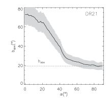
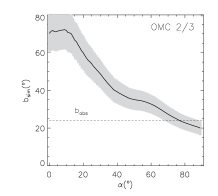
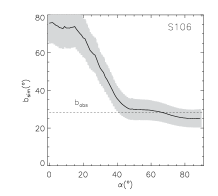
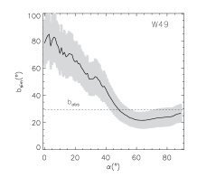
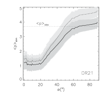
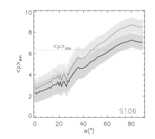
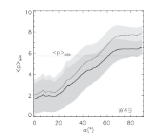
Figure 12.— Top plots: Variations of the turbulent angular dispersion parameter $b_{\rm sim}$ as a function of the inclination angle $\alpha_{\rm sim}$ of the uniform initial magnetic field. The dotted line shows the value $b_{\rm obs}$ obtained from the analysis of the maps of the different regions. Bottom plots: same as top plots but for the mean polarization degree parameter. The black full line shows results obtained with $\epsilon=0.1$; the grey dashed line shows results obtained with $\epsilon=0.12$ (see text for details). Intercepts of curves of $b_{\rm sim}$ and $<p_{\rm sim}>$ (including error bars) with values of $b_{\rm obs}$ and $<p_{\rm obs}>$, respectively, give constraints on values of $\alpha_{\rm sim}$.

4. DISCUSSION

4.1. Shortcomings of the Simulations

Since we focused the modeling of polarization statistics on the turbulent regime of the studied regions we deliberately avoided the use of self-gravity and radiative cooling. For the molecular gas, radiative cooling plays a minor role in the evolution of the turbulent motions and the statistics of the dense structures, and result in very little variations in local temperatures in the range of $T\sim 8-20$K. Self-gravity, on the other hand, plays a major role on the smaller scale dynamics of the molecular clouds, resulting in their fragmentation and collapse of Jeans unstable cores. We tried to remove possible effects of the cores by removing the largest column density pixels out of the statistical study and, as shown before, the parameters $\sigma(\theta)$, $<p>$ and $b$ are only slightly sensitive to that process. In this sense, except for parameter $\gamma$ which will be discussed more in the following, our analysis does not rely on parameters which are too sensitive to the structures of the cloud considered. This can be seen in Figure 11 where variations of parameters $b$, $<p>$ and even $s(\theta)$ are quite smooth as the CDC parameter decreases.

From the point of view of dust grains, our simulations do not take into account possible variations of $p$ with parameters $\lambda$, T_g and $\beta$, i.e. the wavelength of dust grain emission, the dust grain temperature and the dust grain emissivity index, respectively. Variations of dust grains size and / or variations of dust grains axis ratio, whether their shape is oblate or prolate on average, or non ideal, are also not included explicitly. Nevertheless all this infotmation is statistically and implicitly included in the choice of the value for parameter $\epsilon$ used in equation 3.2 to make our numerical calculations. We will see in the next section that a value of $\epsilon\simeq 0.1$ is a reasonable statistical value to describe the turbulent states of the systems investigated.

4.2. Polarization Efficiency Parameter

Two variants of the definition of the polarization efficiency parameter (or polarization reduction factor) have been described and used up to now. They have been mainly proposed by theoreticians based on the fact that the measured linearly polarized signal, as supposed to be produced by layers of aligned dust grains, whether in emission or by dichroic extinction, seems never to exceed a given threshold. In the submm range, which is the domain of wavelengths we are interested, this threshold is often considered to be around a value of 10 $\%$ based on ground-based or airborne experiment observations of sufficiently bright star-forming regions (e.g. Hildebrand et al., 1999), while maxima lying between 10 $\%$ to 20 $\%$ are expected in more diffuse regions of the ISM (see Benoît et al., 2004).

The general definition of the polarization efficiency parameter is given by:

$$\Phi=RF\cos^{2}\gamma_{pos},$$ (13)

where $F$ is the polarization reduction due to the turbulent component of the magnetic field and $\gamma_{pos}$ is the angle between the POS and the local direction of the magnetic field while $R$ is the Rayleigh polarization reduction factor.

In the first variant of the definition provided by Greenberg, (1968), $R$ is defined as:

$$R=1.5(\langle\cos^{2}\beta\rangle-1/3)$$ (14)

where $\beta$ is the angle between the grain angular momentum vector and the magnetic field. In this case $R$ translates as a constant imperfect alignment in the reference frame of each dust grain.

A second definition for $R$ has been proposed by Cho & Lazarian (2005) such that:

$$R=\frac{\int^{a_{\rm max}}_{a_{\rm alg}}C_{\rm ran}n(a)da}{\int^{a_{\rm max}}_{a_{\rm min}}C_{\rm ran}n(a)da},$$ (15)

where, $C_{\rm ran}=(2C_{\perp}+C_{\parallel})/3$ is the dust grain cross section, $a$ is the dust grain size, $n(a)$ is the grain number density, $a_{\rm min}$ is the minimum size, $a_{\rm max}$ is the maximum size, and $a_{\rm alg}$ is the minimum aligned size.

This second definition differs from the first one in the sense that $R$ is now defined as a function of the distribution in size of the grains. Environment effects are very important and the central idea is that non symetrical grains can be radiatively aligned by torques (Radiative Alignment by Torques or RATs, see Hoang and Lazarian et al., 2008) produced by energy transfer on dust grains during their interaction with the Interstellar Radiation Field (ISRF). In particular big grains could be perfectly aligned by this process.

One can now compare those definitions with the assumptions used in and the calculations done with our simulations. Comparison of equations 3.2 and 13 shows that $\gamma_{pos}=90^{\circ}-i$, i.e. all simulated dust grains located in a cell of density $\rho$ are identically aligned by a local magnetic field which orientation makes an angle $\gamma_{pos}$ with the POS. The effects of the turbulence as described by parameter F in equation 13 are directly estimated with our simulations, and the Rayleigh parameter $R$ whether it is described by equation 14 or 15, can therefore be identified to our parameter $\epsilon$ shown in equation 3.2.

In this context our choice of value for $\epsilon$, identified as the maximum polarization degree that could be measured at a given wavelength, should be interpreted as the case where optimal ideal physical conditions are encountered in the ISM. Or in other words, the maximum polarization degree observed at 850 $\mu$m in the SCUPOL catalog would be the maximum value measured if the large scale magnetic field were uniform, lying in a plane almost parallel to the POS and largely dominating over the turbulent field. In such a case we would, therefore, have $\phi\approx\epsilon$.

Following this line of thought we looked into the values of the maximum degree of polarization $p_{\rm max}$ measured on the 4 sources compared with our simulations. All measurements are excessively high with $p_{\rm max}>19\%$ for pixels where the flux density $I$ is each time very low and all corresponding pixels are located on the edges of the clouds. In fact, these estimates of $p_{\rm max}$ look like outliers in the polarization degree distribution which we believe can simply be explained by a high sensitivity of the values of $p=\sqrt{Q^{2}+U^{2}}/I$ in these particular domains of the maps due to the calibration of the intensity maps; i.e. $p$ would be very sensitive to small offsets on $I$ on the edge of the maps. Therefore, we have adopted another approach and checked how the value of $\epsilon=0.1$ compares with the statical maximum $p_{\rm max,stat}\sim<p>+3\times s(p)$ which one could expect for the distributions of $p$ of each sample with the assumption that the distribution of the Stokes parameter is at first order gaussian in nature (e.g. Serkowski et al., 1962). We find values of $p_{\rm max,stat}$ equal to $\approx 7.8\%$, $\approx 9.2\%$, $\approx 8.5\%$ and $\approx 5.4\%$ for regions OMC-2/3, W49, S106 and DR21, respectively, i.e. values which are lower than 10 $\%$. These results do not justify our choice for $\epsilon$, but show that this choice is not inconsistent with the distribution of the polarization degree detected in each region. In addition, the mean turbulent-to-uniform ratios obtained from the SF analyses for those regions all show that the uniform components of the magnetic fields should dominate over the turbulent ones within a factor of 2 to 3, i.e. the magnetic field turbulent component is not expected to constrain $<p>$ to values close to 0, in agreement with the results displayed in Table 1.

On the other hand, a closer look to the SCUPOL catalog and to the results displayed in Table 1 show that values of the mean polarization degree $<p>$ can be found as high as $\approx 10\%$, as in the case for IRAM 04191+1522 and Mon IRAS 12. Therefore, one could expect variations of the polarization efficiency from one region to the other. A look to the plots shown in Figure 12 show that variations of $\epsilon$ should only affect the variations of $<p_{\rm sim}>$ as a function of $\alpha_{\rm sim}$. For illustration purpose, we have added the curves shown with grey dashed-lines obtained for $\epsilon=0.12$ and for each region, except OMC-2/3, we still find common fitting solutions to $\alpha$ from the intercepts of $b_{\rm sim}$ and $<p_{\rm sim}>$ with $b_{\rm obs}$ and $<p_{\rm obs}>$, respectively.

In conclusion, if the physics employed in our simulations to describe the turbulent regimes of the cloud envelopes is correct, as suggested by the results displayed in Table 4, then solutions to $\alpha$ should be firstly constrained from the comparison of $b_{\rm sim}$ with $b_{\rm obs}$. And, on a second round, it would be theoretically possible to constrain a range of solutions to $\epsilon$ by exploring where the intercepts of $<p_{\rm sim}>$ with $<p_{\rm obs}>$ obtain for different values of $\epsilon$ give values of $\alpha$ still consistent with the solutions obtained from the comparison of $b_{\rm sim}$ with $b_{\rm obs}$.

4.3. Comparison with other Works

Cho & Lazarian (2005) show that under peculiar conditions depolarization could occur if grains embedded in dark clouds are aligned by radiative torques (RATs) such that their long axis is perpendicular to the magnetic field. In their model, the mean field is about 2 times stronger than the fluctuating magnetic field, a condition consistent with our results obtained from the analysis of the four regions compared with our simulations. The authors assume a uniform component of the magnetic field to be in the POS, i.e. $\alpha\approx 90^{\circ}$. Their results should be valid for clouds without embedded massive stars.

An application of the definition proposed by Cho & Lazarian (2005) (see equation 15) has been investigated by Pelkonen et al. (2007) with magnetohydrodynamic (MHD) simulations of turbulent supersonic flows distinguishing sub-Alfvénic from super-Alfvénic cases. The inclusion of a proper radiative transfer calculation without detailed simulations of anisotropy shows that alignment efficiency decreases as the RATs become less important into the denser regions. In their work, the question is raised how to distinguish the possible effect of the magnetic field topology from the interception of multiple sources. A possible complication for which likelihood should be avoided is by masking the high density regions as we did in our work. The maximum degree of polarization used by Pelkonen et al. (2007) is fixed to 15$\%$.

An extension of the Cho & Lazarian (2005) model has been proposed by Bethell et al. (2007) by including the effects of the mean Interstellar Radiation Field (ISRF), as well as solutions of the radiative transfer equation to clumpy, optically thick ($A_{\rm V}\sim 10$) prestellar cores and turbulent molecular clouds. Their results are consistent with those described by Cho & Lazarian (2005) and isothermality of large aligned grains is shown to be a reasonable hypothesis. With the Rayleigh reduction factor $R$ defined from equation 15, those authors find that the maximum polarization degree, as well as the power index of the $p-I$ relations are extremely sensitive to the adopted upper cutoff of the power-law distribution of dust grain size, but only moderately sensitive to simplifying assumptions about the radiative anisotropy and no maximum polarization degree is arbitrarily introduced. Despite the highly complex topologies of the magnetic field, those authors show that polarization maps should trace the mass-weighted projected magnetic field vectors reasonably well. Their model explores a large area of parameter space, but does not study the variations of MHD regimes nor consider the impact of embedded sources.

Supplementary analysis on the subject is given by Pelkonen et al. (2009) where an extension of their 2007 work is proposed. In their study they consider $F=1$ and a maximum polarization degree still fixed to 15$\%$. The effect of the distribution of the size of the grains is investigated further away and the effects of the anisotropy of the ISRF are added to the analysis. They find that the inclusion of direction-dependent radiative torque efficiency weakens the dust grains alignment. This effect can be partially counterbalanced if the grain size is doubled in denser regions which means that magnetic fields could theoretically still be probed up to $A_{\rm V}\sim 10$ in regions without embedded sources and where the dynamical timescale of coagulation processes is short enough.

The simulations discussed above cannot be compared directly to ours mainly because they do not explore the same MHD regimes as we do, and also because they are more focused on cloud cores physical characterization rather than on cloud envelopes characterization, as we propose. For example, the turbulent regimes discussed by Pelkonen et al. (2009) are supersonic and super-Alfvénic while the one we find for the envelopes of S106, OMC-2/3, W49 and DR21 are supersonic and sub-Alfvénic. This might also explain the difference on the choice of values for $\epsilon$.

4.4. The Depolarization Parameter

The synthetic polarization maps obtained from the MHD simulations give estimates of $\gamma_{\rm sim}>-0.5$. These values are systematically different from the results obtained from the observed maps, where $\gamma_{\rm obs}<-0.5$. We can therefore speculate what could be the cause of this difference.

One of the main aspects that distinguish simulations and observations is the instrument sensitivity. While in numerical simulations we select the cells we want to use in the statistics, on the observational side the degrees of freedom are much smaller. Low intensity regions of the MHD simulations could be over-represented compared to real data sets because observed LOS low column density cannot be probed from the ground. As pointed in Falceta-Gonçalves et al. (2008), at the lower end of intensity range the simulations reveal no correlation between intensity and polarization degree. The reason for this is that the turbulence in the low intensity regions is basically sub-Alfvenic, i.e. magnetically dominated (see Burkhart et al. 2009). Once we move the statistics to the high intensity regions, the denser regions become more turbulent dominated, resulting in strong depolarization. The turbulent depolarization is a function of the intensity.

From the observational point of view, the limited sensitivity of the instrument biases the statistics for the high intensity regions. It would be theoretically possible to remove low intensity pixels in the simulated maps and produce steeper slopes of the power-law used to fit the $p-I$ relation but how to choose this threshold limit would be too much arbitrary given the shortcomings of the models discussed in section 4.1.

Another possible effect taking part is the alignment efficiency of the dust particles. The numerical simulations do not include radiative alignment for instance. Bethell et al. (2007) and Pelkonen et al. (2009) show that, with the definition of the Rayleigh reduction factor $R$ from equation 15, the maximum polarization degree as well as the power-law index of the $p-I$ relation are extremely sensitive to the adopted cutoff of the power-law distribution of dust grain size and moderately sensitive to symplifying assumptions about the radiative anisotropy, as remarked before. At the same time, as mentionned before, their modelling do not explore the same range of turbulent regimes than we do which limits a direct comparison with our works.

4.5. Interdependence of the Parameters

Every probability distribution function of the polarization degree $p$, PDF($p$), can theoretically be described as a function of the parameter $\Phi$ from equation 13 with the following relation:

$$\rm PDF\it(p)=f(\Phi=RF\cos^{2}\gamma_{pos}).$$ (16)

For each regions, the estimate of $<p>$, is expected to depend on the values of the Rayleigh polarization reduction factor $R$, of the turbulent polarization reduction factor $F$, and on the average inclination of the uniform component of the magnetic field $\gamma_{pos}$. Within our modeling the parameter $\gamma_{pos}$ is directly deduced from the initial conditions of the simulations. The effect of $F$ is directly included in our calculations via the integration of the Stokes parameters along each LOS and estimates of $b$ should only depend on this parameter. In addition, the $p-I$ relation power-law index parameter $\gamma$ should mainly depend on the values of the parameter $R$. This seems to be consistent with the lack of correlation between parameters $p$, $b$ and $\gamma$ discussed in section 2.3.2 and shown in Figures 6, 7 and 8.

On the other hand, if RATs is the dominating mechanism producing dust grain alignment, the interdependence of parameters $p$, $b$ and $\gamma$ might be more complex and for example several cases could be imagined such the that parameter $\gamma$ could depend on the values of $\Phi$ and not $R$ only. Such studies are obviously out of the framework of this work and would need further investigations.

5. SUMMARY AND CONCLUSION

In this work we have presented an extensive analysis of the star-forming and molecular clouds 850 $\mu$m polarization maps of the SCUPOL Catalog produced by Matthews et al. (2009).

For each of the 27 sufficiently sampled regions, sets of parameters $<p>$, $b$ and $\gamma$ are systematically calculated in order to characterize the polarization properties, the depolarization properties and the turbulent-to-mean magnetic field ratio of each region as seen on the POS. As expected from theoretical modelling, the statistical analysis showed no specific correlation between these parameters.

We also created synthetic 2D polarization maps from 3D MHD $1024^{3}$ pixels grid simulations, performed for different MHD regimes, as discussed by Falceta-Gonçalves et al. (2008). Such MHD regimes are estimated for the S106, OMC-2/3, W49 and DR21 molecular cloud regions with 3D MHD cubes properly scaled to the observed maps. The values obtained from the simulations for the Alfvén and sonic Mach numbers are in good agreement, within a factor of 2, with the values obtained for those parameters from Zeeman measurements as estimated by Crutcher (1999) in the same regions.

Constraints on the values of the inclination angle $\alpha$ of the mean magnetic field with respect to the LOS, are obtained by comparing the values of parameters $<p>$ and $b$ estimated from the simulated maps to those obtained from the observed maps of these four regions. Last line of Table 6 gives a summary of the range of estimates obtained for $\alpha$ from our data (1st line), and the constraints provided by Houde (2004) (2nd line) and the range given by the combination of Zeeman measurements and the CF method (lines 3 and 4 of the Table).

Our main conclusion is that most of the results obtained from our analysis of simple ideal isothermal and non-selfgraviting 3D MHD simulations, once properly scaled to the observations, are consistent with results obtained from the latter. This suggests that turbulence only is sufficient to describe the basic dynamical properties of the molecular cloud envelopes, without including the effects of gravity or radiation effects (e.g. in terms of grain alignment).

FOR ACKNOWLEDGEMENTS

We thank the anonymous referee for his comments that helped to improve this work. The research of FP has been supported by the Fundação de Amparo à Pesquisa do Estado de São Paulo (FAPESP no 2007/56302-4). FP also thanks the Leverhulme Trust through the Research Project Grant F/00 407/BN. EDGP thanks the Brazilian agencies FAPESP (no. 2006/50654-3) and CNPq (306598/2009-4) for financial support. DFG thanks the European Research Council (ADG-2011 ECOGAL), and brazilian agencies CNPq (no. 300382/2008-1), CAPES (3400-13-1) and FAPESP (no.2011/12909-8) for financial support.

Table 1Results of the Analysis.

Object	Region(a)	Map	Region(b)	$<p>$ $\pm$ s($(p)$)	$<\theta_{p}>$ $\pm$ s($\theta_{p}$)	$\gamma$	$b$	$\frac{<B^{2}_{t_{||}}>^{1/2}}{B_{0}}$
Name	Type	Pixel	Distance
		Number	(kpc)	($\%$)	$(^{\circ})$		$(^{\circ})$
(1)	(2)	(3)	(4)	(5)	(6)	(7)	(8)	(9)
1 Galactic Center	GC	654	8000.00	2.8 $\pm$ 0.6	142.1$\pm$ 43.7	-0.94 $\pm$ 0.01	24.6$\pm$ 1.5	0.32$\pm$ 0.02
5 AFGL333	SFR	233	1.950	8.2 $\pm$ 1.2	001.3$\pm$ 38.1	-1.00 $\pm$ 0.05	21.1 $\pm$ 1.5	0.27$\pm$ 0.02
8 NGC1333	SFR	193	0.320	6.2 $\pm$ 0.9	055.1$\pm$ 47.1	-0.26 $\pm$ 0.02	35.1 $\pm$ 1.5	0.48$\pm$ 0.02
9 Barnard 1	SFR	101	0.250	6.2 $\pm$ 1.0	054.9$\pm$ 41.2	-0.83 $\pm$ 0.05	37.5 $\pm$ 1.4	0.52$\pm$ 0.02
11 OMC-1	SFR	385	0.414	4.0 $\pm$ 0.6	155.4$\pm$ 38.7	0.10 $\pm$ 0.01	14.8 $\pm$ 1.4	0.19$\pm$ 0.02
12 OMC-2/3	SFR	361	0.414	4.8 $\pm$ 1.0	079.5$\pm$ 41.5	-0.63$\pm$ 0.01	24.2 $\pm$ 1.1	0.31$\pm$ 0.02
13 NGC 2024	SFR	203	0.400	4.1 $\pm$ 0.8	092.1$\pm$ 38.5	-0.84$\pm$ 0.03	14.4 $\pm$ 1.7	0.18$\pm$ 0.02
15 NGC 2068	SFR	285	0.400	7.0 $\pm$ 0.9	039.3$\pm$ 39.4	-0.75$\pm$ 0.04	35.1 $\pm$ 1.4	0.48$\pm$ 0.02
18 Mon R2 IRS1	SFR	183	0.950	4.9 $\pm$ 0.9	072.4$\pm$ 30.7	-1.16$\pm$ 0.03	21.9$\pm$ 1.7	0.28$\pm$ 0.02
20 Mon IRAS 12	SFR	171	0.800	9.9 $\pm$ 2.1	049.7 $\pm$ 45.8	-0.86 $\pm$ 0.03	44.5$\pm$ 1.1	0.66$\pm$ 0.02
22 rho Oph A	SFR	337	0.139	5.3 $\pm$ 0.9	063.2$\pm$ 39.8	-0.80$\pm$ 0.02	21.8 $\pm$ 1.5	0.28$\pm$ 0.02
24 rho Oph B2	SFR	113	0.139	5.3 $\pm$ 1.1	056.6$\pm$ 45.1	-0.86$\pm$ 0.06	36.2$\pm$ 1.3	0.50 $\pm$ 0.02
25 NGC 6334A	SFR	77	1.700	4.2 $\pm$ 1.0	094.8$\pm$ 43.2	-0.82$\pm$ 0.05	14.5 $\pm$ 1.7	0.18$\pm$ 0.02
26 G011.11-0.12	SFR	143	3.600	5.4 $\pm$ 1.2	134.7$\pm$ 26.7	-0.89$\pm$ 0.03	25.3$\pm$ 1.6	0.33$\pm$ 0.02
27 GGD 27	SFR	49	1.700	6.7 $\pm$ 1.6	178.1$\pm$ 39.9	-0.82$\pm$ 0.06	37.3 $\pm$ 1.5	0.52$\pm$ 0.03
29 Serpens Main Core	SFR	231	0.310	7.1 $\pm$ 1.4	075.3$\pm$ 40.4	-1.01$\pm$ 0.03	36.8$\pm$ 1.3	0.51$\pm$ 0.02
33 W48	SFR	122	3.400	4.9 $\pm$ 1.0	152.3$\pm$ 44.2	-0.59 $\pm$ 0.02	35.7 $\pm$ 1.3	0.49$\pm$ 0.02
35 W49	SFR	368	11.400	5.3 $\pm$ 1.3	108.5$\pm$ 45.5	-0.83$\pm$ 0.01	29.6 $\pm$ 1.2	0.39$\pm$ 0.02
36 W51	SFR	123	7.500	3.2 $\pm$ 0.8	137.5$\pm$ 50.5	-0.71$\pm$ 0.03	34.0$\pm$ 1.4	0.46$\pm$ 0.02
41 S106	SFR	201	0.600	5.8 $\pm$ 0.9	115.7$\pm$ 47.1	-0.78$\pm$ 0.03	28.4$\pm$ 1.4	0.37$\pm$ 0.02
43 DR21	SFR	439	3.000	3.6 $\pm$ 0.6	077.0$\pm$ 35.9	-0.50$\pm$ 0.01	19.3 $\pm$ 1.8	0.25$\pm$ 0.02
47 S152	SFR	123	5.000	5.6$\pm$ 1.0	081.8$\pm$ 34.3	-0.61$\pm$ 0.04	21.2 $\pm$ 1.8	0.27$\pm$ 0.02
50 L1448	YSO	130	0.250	5.1 $\pm$ 1.0	040.3$\pm$ 47.5	-0.87$\pm$ 0.04	41.1 $\pm$ 1.4	0.59$\pm$ 0.03
53 L1527	YSO	92	0.140	6.6 $\pm$ 1.3	101.4 $\pm$ 38.7	-1.10$\pm$ 0.05	37.4 $\pm$ 1.3	0.52$\pm$ 0.02
54 IRAM 04191+1522	YSO	55	0.140	10.6 $\pm$ 2.5	074.5 $\pm$ 35.3	-1.35$\pm$ 0.09	35.2$\pm$ 1.3	0.48$\pm$ 0.02
59 Cep A	YSO	100	0.730	4.6 $\pm$ 1.0	127.6 $\pm$ 44.1	-0.65$\pm$ 0.03	15.8 $\pm$ 1.5	0.20$\pm$ 0.02
66 L43	SPC	40	0.170	7.2 $\pm$ 1.6	134.9$\pm$ 37.3	-1.44$\pm$ 0.14	33.1 $\pm$ 1.4	0.45$\pm$ 0.02

Table 2Sample Statistics.

Sample	Objects	$\overline{<p>}$	$\overline{\gamma}$	$\overline{s(\theta_{p})}$	$\overline{b}$
	Number	$(\%)$		(∘)	(∘)
All Selected Regions	27	5.72 $\pm$ 1.84	-0.81 $\pm$ 0.30	40.7 $\pm$ 5.4	28.7$\pm$ 8.9
Galactic Center	1	2.77 $\pm$ 0.00	-0.94 $\pm$ 0.00	43.7 $\pm$ 0.0	24.6$\pm$ 0.0
SFRs(a)	21	5.59 $\pm$ 1.59	-0.74 $\pm$ 0.27	40.6 $\pm$ 5.7	28.0$\pm$ 8.9
YSOs(a)	4	6.73 $\pm$ 2.72	-0.99 $\pm$ 0.30	41.4 $\pm$ 5.4	32.4$\pm$ 11.3
SPCs(a)	1	7.23 $\pm$ 0.00	-1.44 $\pm$ 0.00	37.3 $\pm$ 0.0	33.1$\pm$ 0.0

Table 3Total Magnetic Fields Intensities and Inclinations.

Object	$B_{\rm LOS}^{(a)}$	log $n^{(a)}$	$\sigma_{v}^{(a)}$	$B_{\rm POS}^{HIL09}$	$B_{\rm POS}^{FLK08}$	Map Areas Ratio	$\alpha_{(\rm max)}^{(b)}$
Name	($\mu$G)	(H2 cm-3)	(km/s)	($\mu$G)	($\mu$G)	(pol./spectro.)	(∘)
OMC-1	360	5.9 (5.9)(c)	0.60 (1.85)(c)	1976 (6149)(d)	395 (1229)(d)	$\sim$ 33	79.7 (86.6)(d)
NGC 2024	87	5.0 (5.0)(c)	0.64 (0.68)(c)	773 (830)(d)	154 (165)(d)	$\sim$ 2	83.6 (84.0)(d)
$\rho$ Oph. A (1(a))	10	3.0 (5.0)(c)	0.55 (0.58)(c)	43 (455)(d)	8 (84)(d)	$\sim$ 1	77.0 (88.7)(d)
$\rho$ Oph. B2 (2(a))	14	3.2	0.59	33	2	$\sim$ 1	66.9
W49	21	3.0	0.64	36	$1-2$	$\sim$ 0.1	59.4
S106	400	5.3	0.68	562	19	$\sim$ 16	54.6
DR21 (OH1(a))	710	6.3 (6.3)(c)	0.98 (2.04)(c)	3897 (8140)(d)	1210 (2528)(d)	$\sim$ 26	79.7 (85.0)(d)
DR21 (OH2(a))	360	6.0 (6.0)(c)	0.98 (2.04)(c)	2759 (5762)(d)	856 (1789)(d)	$\sim$ 26	82.6 (86.4)(d)

Table 4Description of the Simulations - MHD, 1024³.

Model	$M_{S}^{(a)}$	$M_{A}^{(b)}$	Object Name	$M_{S}^{(c)}$	$M_{A}^{(c)}$
1……….	2.0	0.3	S106	3.6	0.2
2……….	3.0	0.5	OMC-2/3	-	-
3……….	5.0	0.7	W49	5.9	0.6
4……….	5.0	0.7	DR21	4.0 (4.0)	1.3 (1.8)(d)

Table 5Parameter extracted from the analysis of the observed maps for comparing with simulated maps.

Region	Cloud size	Obs. resolution	CDC cut(a)	Fraction of rejected	$b$	$\gamma$	$P$	s$(\theta_{p})$
Name	(pc$\times$pc)	(pc)	$(\%)$	pixels	$(^{\circ})$		$(\%)$	$(^{\circ})$
S106	$\sim$ 0.9 $\times$ 0.6	$\sim$ 0.03	85.3	25/201	$\sim$ 28.4 $\pm$ 1.4	-0.91 $\pm$ 0.05	6.3 $\pm$ 3.4	47.3
OMC-2/3	$\sim$ 2.2 $\times$ 0.4	$\sim$ 0.04	94.9	19/361	24.1 $\pm$ 1.1	-0.86 $\pm$ 0.02	4.9 $\pm$ 4.4	42.3
W49	$\sim$ 16.6 $\times$ 9.9	$\sim$ 0.55	95.4	36/368	$\sim$ 29.6 $\pm$ 1.2	-1.05 $\pm$ 0.01	5.7 $\pm$ 5.7	44.7
DR21	$\sim$ 4.4 $\times$ 2.6	$\sim$ 0.15	95.9	27/439	$\sim$ 19.3 $\pm$ 1.8	-0.63 $\pm$ 0.02	3.7 $\pm$ 2.8	34.1

Table 6Mean Magnetic Field Inclination Angle Summary Table.

Region Name	S106	OMC-2/3	W49	DR21
$\alpha_{\rm sim}(\epsilon=0.10)$ (${}^{\circ})$ (Envelopes)	[50-70]	$>$70	[50-85]	$>$60
$\alpha_{\rm Ion/Neutral}$ (${}^{\circ})$ (Cores)	…	[72-80] (a)	…	[55-70](b)
$\alpha_{\rm CF(CO)+Zeeman}$ (${}^{\circ})$ (Cores + envelopes)	$<$55	…	$<$ 60	$<$ 83
$\alpha_{\rm CF(H^{13}CO^{+}(J=3-2))+Zeeman}$ (${}^{\circ})$ (Cores + envelopes)	…	…	…	$<$ 87
$\alpha_{\rm AllMethods}(\epsilon=0.10)$ (${}^{\circ})$	[50-55]	[72-80]	[50-60]	[60 - 70]

References

- Anderson (2012) Andersson, B.G. 2012, arXiv:1208.4393, to appear in ”Magnetic Fields in Diffuse Media”, A. Lazarian & E.M. de Gouveia Dal Pino eds
- Armstrong, Rickett & Spangler (1995) Armstrong, J. W., Rickett, B. J., & Spangler, S. R. 1995, ApJ, 443, 209
- Bethell et al. (2007) Bethell, T.J., Chepurnov, A., Lazarian, A. & Kim, J. 2007, ApJ, 663, 1055
- Benoît et al. (2004) Benoît, A., Ade, P., Amblard, A. et al. 2004, A&A, 424, 571.
- Burkhart et al. (2009) Burkhart, B., Falceta-Gonçalves, D., Kowal, G. & Lazarian, A. 2009, ApJ, 693, 250