Excitons in quantum dot molecules: Coulomb coupling, spin-orbit effects and phonon-induced line broadening

Abstract

Excitonic states and the line shape of optical transitions in coupled quantum dots (quantum dot molecules) are studied theoretically. For a pair of electrically tunable, vertically aligned quantum dots we investigate the coupling between spatially direct and indirect excitons caused by different mechanisms such as tunnel coupling, Coulomb coupling, coupling due to the spin-orbit interaction and coupling induced by a structural asymmetry. The peculiarities of the different types of couplings are reflected in the appearance of either crossings or avoided crossings between direct and indirect excitons, the latter ones being directly visible in the absorption spectrum. We analyze the influence of the phonon environment on the spectrum by calculating the line shape of the various optical transitions including contributions due to both pure dephasing and phonon-induced transitions between different exciton states. The line width enhancement due to phonon-induced transitions is particularly pronounced in the region of an anticrossing and it strongly depends on the energy splitting between the two exciton branches.

I Introduction

Structures consisting of two closely spaced quantum dots (QDs) have attracted much interest in the past years both in experimentBayer et al. (2001); Krenner et al. (2005); Stinaff et al. (2006); Bracker et al. (2006); Robledo et al. (2008); Goryca et al. (2009); Shulman et al. (2012) and in theory.Bester et al. (2004); Schliwa et al. (2001); Szafran et al. (2005); Szafran (2008); Gawarecki et al. (2010) Carriers in these nanostructure are not strictly confined to one dot but may be delocalized over both dots, which is often described in terms of a tunnel coupling between the individual dots.Bryant (1993); Bracker et al. (2006); Scheibner et al. (2008) This coupling causes the formation of bonding and anti-bonding states in the double dot systems, hence they are often referred to as quantum dot molecules (QDMs). External fields can be used to effectively manipulate carrier localizationsKrenner et al. (2005); Ortner et al. (2005) and to characterize different exciton states,Ortner et al. (2003); Lyanda-Geller et al. (2004); Ortner et al. (2005); Müller et al. (2011); Heldmaier et al. (2012) which is essential for many applications.

Since QDs are embedded in a solid state matrix, the crystal environment plays a crucial role in the carrier kinetics in a QDM. Phonons provide a source of dephasing in single QDsTakagahara (1999); Krummheuer et al. (2002) as well as in coupled QDs.Borri et al. (2003); Stavrou and Hu (2005) They give rise to the relaxation of the exciton, although this is restricted by the phonon bottleneck effect.Benisty (1995) But even if transition rates are strongly reduced because of the lack of final states in the energy region where the coupling to phonons is efficient, phonon-induced pure dephasing has a pronounced influence on the line shape of absorption or emission spectra.Besombes et al. (2001); Krummheuer et al. (2002) For a QDM also phonon-mediated relaxation between bonding and anti-bonding states as well as phonon-assisted tunneling or interdot relaxation may take place.López-Richard et al. (2005); Vorojtsov et al. (2005); Wu et al. (2005); Grodecka et al. (2008); Gawarecki et al. (2010); Gawarecki and Machnikowski (2012)

Experimental studies of exciton spectra in QDMs placed in an axial electric field show characteristic features that are qualitatively different from the quantum confined Stark shift behavior observed in individual QDs. The most pronounced features emerging in the QDM spectra are resonances (anticrossings) that appear at certain intersections between spatially direct and indirect exciton states (that is, states with the electron and the hole residing in the same QD or in different QDs, respectively).Scheibner et al. (2008); Müller et al. (2011) Recent experiments investigated also the phonon-assisted interdot tunneling between the direct and indirect configurations.Müller et al. (2012) Additionally, it was shown, that the phonon-induced relaxation time of an exciton at a tunnel-resonance (anticrossing) exhibits an oscillatory behavior due to an interplay between the phonon wavelength and the distance between the dots.Wijesundara et al. (2011); Rolon et al. (2012) Theoretical modeling of exciton states in QDMs reproduces the observed spectral features, including the structure of the lowest-energy states Szafran et al. (2001) and their behavior in an axial electric field,Sheng and Leburton (2002); Janssens et al. (2002) as well as the tunnel-related anticrossings between the spatially direct and indirect configurations as a function of the electric field, where the crucial role is played by the electron-hole Coulomb interaction.Szafran et al. (2005, 2007); Szafran (2008) Couplings induced by the spin-orbit coupling (SOC) have been studied in laterally coupled quantum dots.Stano and Fabian (2005) Several theoretical studies have also addressed phonon-related processes in QDMs, focussing on single- López-Richard et al. (2005); Vorojtsov et al. (2005); Wu et al. (2005); Gawarecki et al. (2010) and two-electron Gawarecki et al. (2010); Grodecka et al. (2008) as well as single-hole systems Gawarecki and Machnikowski (2012) and excitons.Muljarov et al. (2005)

In this paper, we present a systematic study of excitons in QDM structures, which are tunable by an external electric field. We extend previous research by investigating avoided exciton level-crossing mediated by Coulomb coupling with higher exciton states. We also consider couplings between exciton states with different values of the angular momentum which can be induced either by the SOC or by a breaking of the cylindrical symmetry of the confinement potential. To calculate the line shape of the transitions in the absorption spectrum we take into account the coupling to acoustic phonons including both the phenomena of pure dephasing as well as phonon-induced transitions to other exciton states.

From our calculations we find that Coulomb interaction is crucial for understanding the sequence of exciton states and tunnel resonances. We show that besides modifying the sequence of the states the Coulomb interaction also leads to the appearance of additional anticrossings between two configurations in which not only one of the carriers (electron or hole) resides in different dots but also the other carrier is in different states within one dot. Such two-particle states are not connected by the usual single-particle tunneling and, therefore, would not give rise to a resonant anticrossing in the absence of the off-diagonal part of the Coulomb coupling. The effective coupling between the two states forming such a resonance is found to be of comparable magnitude as the usual tunnel coupling. For the combined system of exciton and phonons, we investigate phonon-assisted tunneling and the line shape of absorption as a function of temperature. In addition, we study the effect of the SO coupling in the area of level crossings (corresponding to the degeneracy points between states of different angular momentum). We show that it leads to a qualitative change of the system spectrum by opening a resonant anticrossing between spin-bright and spin-dark states with different angular momenta. A comparable effect can be caused by a misalignment of the dots or by deviations from a rotational symmetry of the QDs, which breaks the conservation of angular momentum.

The paper is organized as follows: In Sec. II we summarize the underlying theory of the calculations. We start with the model for the carrier wave-functions and the exciton states. Then, the coupling of the exciton to the phonon system is described and a Green’s function formalism for the calculation of absorption spectra is introduced, followed by the introduction of spin-orbit coupling. In the same way the results are presented in Sec. III. We start with the exciton energy-level structure and a discussion of the absorption spectra of a typical QDM. Then, different types of crossing and avoided crossings are discussed as well as the impact of the phonon environment. Finally the coupling between excitons states with different angular momentum either due to the SOC or due to a broken cylindrical symmetry of the confinement potential is discussed. The paper concludes with a brief summary and some final remarks in Sec. IV.

II Model

II.1 Exciton States

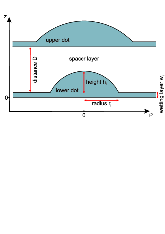
Figure 1: (Color online) Sketch of the quantum dot molecule.

We consider a QDM formed by two vertically stacked QDs of a lens-like shape in a GaAs matrix. The QDs are modeled as spherical segments of In_xGa_1-xAs with homogenous indium fraction $x$, base radii $r_{i}$ and heights $h_{i}$ on thin wetting layers of thickness $w_{i}$ (see Fig. 1). The QDs are centered at $\rho=0$ of a cylindrical coordinate system with the coordinates $(\rho,\phi,z)$. The confinement potential for electrons and holes is given by the band edge discontinuity of conduction and valence band, respectively, between the QD and the host material. The confined electron (hole) states are calculated within a variational multicomponent envelope function scheme as has been presented in detail in Ref. Gawarecki et al., 2010. In this scheme, an “adiabatic” approximation of the single-particle wave functions $\psi^{l,M}(\rho,z,\phi)$ is used (cf. Ref. Wojs et al., 1996). We use the trial functions

$$\psi^{l,M}(\rho,z,\phi)=\frac{1}{\sqrt{2\pi}}\sum_{\alpha}\chi_{\alpha}(z;\rho)\varphi^{l,M}_{\alpha}(\rho)\text{e}^{iM\phi},$$ (1)

where $M$ is the quantum number describing the projection of the angular momentum on the $z$-direction, and $l$ is another quantum number that uniquely labels the states with a given angular momentum. The functions $\chi_{\alpha}(z;\rho)$ are the solutions of the one-dimensional Schrödinger equation of the double well potential along the $z$-direction for a fixed $\rho$,

$$\left\{-\frac{\hbar^{2}}{2m_{\text{c/v}}}\frac{\partial^{2}}{\partial z^{2}}+E_{\text{c/v}}(z;\rho)\right\}\chi_{\alpha}(z;\rho)=E_{\alpha}(\rho)\chi_{\alpha}(z;\rho),$$ (2)

representing the subbands of the confined states in the double well. Here, $E_{\text{c/v}}(z;\rho)=V_{\text{c/v}}(z;\rho)+V(z)$ is the effective confinement potential consisting of the confinement potential $V_{\text{c/v}}(z;\rho)$ resulting from the band edge discontinuities of the conduction/valence band and the potential $V(z)$ of the external electric field.note (2013) From the potential along the $z$-direction, we take the lowest three confined states into account. Because the confinement potential of the dots varies slowly with $\rho$, in Eq. (1), $\varphi^{l,M}_{\alpha}(\rho)$ is a slowly varying envelope function for this coordinate. The lowest $\psi^{l,M}$-states can be obtained by applying Ritz’ variational method and minimizing the energy functional $F[\psi^{l,M}]$ within the class of trial functions defined in Eq. (1),

$$F[\psi^{l,M}] = \langle\psi^{l,M}\left|H\right|\psi^{l,M}\rangle=\sum_{\alpha,\beta}\int^{\infty}_{0}\int^{\infty}_{-\infty}\rho\frac{\hbar^{2}}{2m}$$ (3)

$$\times\frac{\text{d}}{\text{d}\rho}\left(\chi_{\alpha}(z;\rho)\varphi^{l,M}_{\alpha}(\rho)\right)^{*}\frac{\text{d}}{\text{d}\rho}\left(\chi_{\beta}(z;\rho)\varphi^{l,M}_{\beta}(\rho)\right)\text{d}\rho\text{d}z$$

$$+\sum_{\alpha}\int^{\infty}_{0}\varphi^{l,M^{*}}_{\alpha}(\rho)\left(E_{\alpha}(\rho)+\frac{\hbar^{2}M^{2}}{2m\rho^{2}}\right)\varphi^{l,M}_{\alpha}(\rho)\rho\text{d}\rho$$

$$-\lambda\left(\sum_{\alpha}\int_{0}^{\infty}\varphi_{\alpha}^{l,M^{*}}(\rho)\varphi_{\alpha}^{l,M}(\rho)\rho\text{d}\rho-1\right),$$

where $\lambda$ is a Lagrange multiplier introduced to enforce normalization. This minimization can be converted into an eigenvalue problem with $\lambda$ becoming the energy eigenvalues, i.e., $\epsilon^{\text{e}}_{i}$ ($\epsilon^{\text{h}}_{j}$) for the electron (hole) energies, where $i$ ($j$) is a multi-index including both quantum numbers $l$ and $M$.

The single-particle functions of electron and hole found in this way are used to calculate the exciton states within a configuration interaction scheme. For this purpose, we take the space spanned by the products of the single-particle states, i.e. $\tilde{\Psi}_{ij}=\psi^{\text{e}}_{i}\psi^{\text{h}}_{j}$, as a basis. Including the Coulomb interaction between electron and hole, the Hamiltonian in this basis reads

$$H_{\text{exc}} = \sum_{i}\epsilon^{\text{e}}_{i}c^{\dagger}_{i}c^{\phantom{\dagger}}_{i}+\sum_{j}\epsilon^{\text{h}}_{j}d^{\dagger}_{j}d^{\phantom{\dagger}}_{j}+\sum_{ijkl}v_{ijkl}c^{\dagger}_{i}d^{\dagger}_{j}d^{\phantom{\dagger}}_{k}c^{\phantom{\dagger}}_{l},$$ (4)

where $c^{\phantom{\dagger}}_{i},c^{\dagger}_{i}$ denote the annihilation and creation operators for the electron and $d^{\phantom{\dagger}}_{j},d^{\dagger}_{j}$ likewise for the hole, while $\epsilon^{\text{e}}_{i}$ and $\epsilon^{\text{h}}_{j}$ are the corresponding single-particle energies. The interaction between both particles is described by the last term of the Hamiltonian, with

$$v_{ijkl} = -\frac{e^{2}}{4\pi\varepsilon_{0}\varepsilon_{r}}$$

$$\times\int\int{\psi_{i}^{\text{e}}}^{*}(\textbf{r}){\psi_{j}^{\text{h}}}^{*}(\textbf{r}^{\prime})\frac{1}{|\textbf{r}-\textbf{r}^{{}^{\prime}}|}{\psi_{k}^{\text{h}}}(\textbf{r}^{\prime}){\psi_{l}^{\text{e}}}(\textbf{r})\text{d}^{3}{r}\text{d}^{3}{r}^{{}^{\prime}},$$

where $e$ is the elementary charge, $\varepsilon_{0}$ is the vacuum permittivity, and $\varepsilon_{r}$ is the dielectric constant. This Hamiltonian is diagonalized numerically within a truncated basis leading to

$$H_{\text{exc}}=\sum_{n}\epsilon_{n}\left|X_{n}\right\rangle\left\langle X_{n}\right|,$$ (6)

where the exciton energy $\epsilon_{n}$ corresponds to the state

$$\left|X_{n}\right\rangle=\sum_{ij}a^{n}_{ij}c^{\dagger}_{i}d^{\dagger}_{j}\left|0\right\rangle,$$ (7)

expressed as a superposition of the uncoupled electron-hole pair states with expansion coefficients $a^{n}_{ij}$.

II.2 Exciton-phonon coupling

The excitons in the QDM are coupled to the phononic environment of the structure. Because we are mainly interested in exciton states in an energy range of less than 10 meV and we will consider only low temperatures, we can restrict ourselves to the interaction with acoustic phonons which, due to the very similar elastic properties of the QDs and the surrounding material, can be treated as bulk-like. In QDs, due to the rather large splitting between different confined energy levels, the coupling to acoustic phonons typically gives rise to pure dephasing resulting in a strongly non-Lorentzian line shape of absorption or emission lines Besombes et al. (2001); Krummheuer et al. (2002) consisting of a narrow zero-phonon line (ZPL) superimposed on a broad phonon background. Here, depending on the geometry of the QDM and the external field, some exciton states may come energetically close such that transitions between different excitonic states associated with the emission or absorption of an acoustic phonon become possible, which gives rise to an additional Lorentzian broadening of the ZPLs.

The coupling of the single carriers (electron and hole) to the phonon environment can be described by the generic Hamiltonian

$$H_{\text{c-ph}} = \sum_{s,{\textbf{q}}}\left(\sum_{ij}c^{\dagger}_{i}c^{\phantom{\dagger}}_{j}F^{\text{e}}_{s,ij}({\textbf{q}})+\sum_{kl}d^{\dagger}_{k}d^{\phantom{\dagger}}_{l}F^{\text{h}}_{s,kl}({\textbf{q}})\right)$$ (8)

$$\times\left(b^{\phantom{\dagger}}_{s,{\textbf{q}}}+b^{\dagger}_{s,-{\textbf{q}}}\right).$$

Here, $F^{\text{e/h}}_{s,ij}({\textbf{q}})$ are the carrier-phonon coupling constants between the single-particle states ($i,j$) and a phonon of branch $s$ and momentum q which is described by the boson operators $b^{\phantom{\dagger}}_{s,{\textbf{q}}}$ and $b^{\dagger}_{s,{\textbf{q}}}$. The carriers are coupled to transverse acoustic (TA) phonons via the piezoelectric (PE) coupling and to longitudinal-acoustic (LA) phonons via the PE and the deformation-potential (DP) coupling. The coupling constants $F^{\text{e/h}}_{s,ij}({\textbf{q}})=g^{\text{e/h}}_{s}({\textbf{q}})\mathcal{F}^{\text{e/h}}_{ij}({\textbf{q}})$ are composed of two parts. While the second term

$$\mathcal{F}^{\text{e/h}}_{ij}({\textbf{q}}) = \int{\psi^{\text{e/h}}_{i}}^{*}(\textbf{r})\text{e}^{i{\textbf{q}}\cdot\textbf{r}}\psi^{\text{e/h}}_{j}(\textbf{r})\text{d}^{3}r,$$ (9)

is determined by the envelope functions of the involved states, the first part $g^{\text{e/h}}_{s}({\textbf{q}})$ is the bulk coupling matrix element depending on the specific mechanism. The bulk DP coupling constants are given by

$$g^{\text{e/h}}_{\text{LA}}({\textbf{q}}) = \sqrt{\frac{\hbar q}{2\rho Vv_{\text{LA}}}}a_{\text{c/v}},$$ (10)

where $\rho$ is the crystal density, $V$ is the system volume, $v_{\text{LA}}$ is the speed of sound of the LA phonons, and $a_{\text{c/v}}$ is a deformation potential for the conduction or valence band. The piezoelectric interactions can be described by the constants

$$g^{\text{e/h}}_{s}({\textbf{q}}) = -i\sqrt{\frac{\hbar}{2\rho Vv_{s}q}}\frac{d_{p}e}{\epsilon_{0}\epsilon_{r}}M_{s}(\hat{{\textbf{q}}}),$$ (11)

with $v_{s}$ being the speed of sound of the LA and the TA phonons, respectively, while $d_{p}$ is the piezoelectric constant. $M_{s}(\hat{{\textbf{q}}})$ describes the dependence of the PE coupling on the direction $\hat{{\textbf{q}}}=\frac{{\textbf{q}}}{q}$ of the phonon wave-vector and is given by

$$M_{s}(\hat{{\textbf{q}}}) = 2\left[\hat{q}_{x}(\hat{e}_{s,{\textbf{q}}})_{y}\hat{q}_{z}+\hat{q}_{y}(\hat{e}_{s,{\textbf{q}}})_{z}\hat{q}_{x}+\hat{q}_{z}(\hat{e}_{s,{\textbf{q}}})_{x}\hat{q}_{y}\right],\qquad$$ (12)

where $\hat{e}_{s,{\textbf{q}}}$ is the unit polarization vector for the phonon branch $s$ and the wave vector q.

The interaction of an exciton with the phonon environment is given by the projection of $H_{\text{c-ph}}$ on the exciton states

$$H_{\text{x-ph}} = \sum_{nm}\sum_{s,{\textbf{q}}}F_{s,nm}^{\text{x}}({\textbf{q}})\left(b^{\phantom{\dagger}}_{s,{\textbf{q}}}+b^{\dagger}_{s,-{\textbf{q}}}\right)\left|X_{n}\right\rangle\left\langle X_{m}\right|,\quad$$ (13)

with the exciton-phonon coupling constant

$$F_{s,nm}^{\text{x}}({\textbf{q}}) = \sum_{ij}\left\langle X_{n}\right|c^{\dagger}_{i}c^{\phantom{\dagger}}_{j}\left|X_{m}\right\rangle F^{\text{e}}_{s,ij}({\textbf{q}})$$ (14)

$$+\sum_{kl}\left\langle X_{n}\right|d^{\dagger}_{k}d^{\phantom{\dagger}}_{l}\left|X_{m}\right\rangle F^{\text{h}}_{s,kl}({\textbf{q}}).$$

Since the exciton states are superpositions of electron-hole configurations, this may give rise to transitions between exciton states. The transition rate $\gamma_{nm}$ for a transition between an initial exciton-state $n$ and a final state $m$ with energies $E_{n}$ and $E_{m}$, respectively, is given by Fermi’s golden rule

$$\gamma_{nm}=\frac{2\pi}{\hbar^{2}}\left[n_{\text{B}}(T,\omega_{nm})+\delta\right]J_{nm}(\omega_{nm}),$$ (15)

where $\Delta E_{nm}=\hbar\omega_{nm}=|E_{n}-E_{m}|$, $n_{\text{B}}(T,\omega_{nm})$ is the Bose distribution at the lattice temperature $T$, and $\delta=0$ in case of a phonon absorption (i.e., $E_{m}>E_{n}$) and $\delta=1$ in case of a phonon emission (i.e., $E_{m}<E_{n}$). The phonon spectral density $J_{nm}(\omega)$ for the transition from state $n$ to state $m$ is defined as

$$J_{nm}(\omega) = \sum_{s,{\textbf{q}}}\delta(\omega-\omega_{s,{\textbf{q}}})\left|F_{s,nm}^{\text{x}}({\textbf{q}})\right|^{2}.$$ (16)

The transition rate between two states depends on the applied field, as the energy difference and the wave functions of the involved states are affected by the field. The total decay rate $\gamma_{n}$ of an exciton state $n$ is given by the sum over all possible transitions, $\gamma_{n}=\sum_{m}\gamma_{nm}$. The lifetime $\tau_{n}$ of the state is then defined by the inverse of the transition rate, $\tau_{n}=\gamma_{n}^{-1}$.

II.3 Absorption Spectrum

To investigate the absorption spectrum of the double quantum dot system we consider the dipole coupling of the carriers to a classical light field within the rotating wave approximationRossi and Kuhn (2002); Binder et al. (1994)

$$H_{\text{c-l}}=-\sum_{ij}\textbf{M}_{ij}\cdot\textbf{E}^{(-)}c^{\phantom{\dagger}}_{i}d^{\phantom{\dagger}}_{j}+\text{h.c.},$$ (17)

where $\textbf{E}^{(-)}$ is the negative frequency part of the field and $\textbf{M}_{ij}$ is the dipole matrix element of the interband transition, which is given by the product of the bulk dipole matrix element $\textbf{M}_{0}$ and the overlap integral between electron and hole envelope wave functions. The linear absorption spectrum is proportional to the imaginary part of the linear susceptibility $\chi(\omega)$,Fox (2001) it can therefore be obtained from the projection of the dipole operator on the direction of the light field ${P}=\sum_{ij}{M}_{ij}c^{\phantom{\dagger}}_{i}d^{\phantom{\dagger}}_{j}=\sum_{n}{M}_{n}\left|0\right\rangle\left\langle X_{n}\right|=\sum_{n}{M}_{n}a_{n}$, where $a_{n}$ are the exciton annihilation operators and ${M}_{n}$ the corresponding dipole matrix elements. For a weak, ultra-fast pulse (linear response) at $t=0$, i.e., $E(t)=E_{0}\delta(t)$ one gets Suna (1964); Jacak et al. (2005, 2005) $\langle\langle P(t)\rangle\rangle\sim\chi(t)E_{0}$ with

$$\chi(t) \sim \Theta(t)\sum_{nm}{M}_{n}{M}^{*}_{m}\langle\langle a^{\phantom{\dagger}}_{n}(t)a^{\dagger}_{m}\rangle\rangle$$ (18)

$$= \sum_{nm}{M}_{n}{M}^{*}_{m}G_{n,m}(t).$$

Here, $\langle\langle\dots\rangle\rangle$ is the grand canonical average, which is temperature dependent because of the phonon degrees of freedom. We calculate the polarization by utilizing the single-particle Green’s function $G_{n,m}(\omega)=\int^{\infty}_{-\infty}G_{n,m}(t)e^{i\omega t}{\mathrm{d}t}$. Up to the second order in the phonon coupling and neglecting phonon-induced energy shifts $G_{n,m}(\omega)$ can be approximated byJacak et al. (2005)

$$G_{n,m}(\omega)=\frac{\delta_{n,m}}{\omega-\frac{\epsilon_{n}}{\hbar}+i\tilde{\gamma}_{n}(\omega)}$$ (19)

with the imaginary part of the self-energy

$$\tilde{\gamma}_{n}(\omega)=\sum_{l}\tilde{\gamma}_{nl}(\omega)$$ (20)

and

$$\tilde{\gamma}_{nl}(\omega) = \frac{\pi}{\hbar^{2}}\sum_{s,{\textbf{q}}}\left|F_{s,nl}^{\text{x}}({\textbf{q}})\right|^{2}$$

$$\times\left\{n_{\text{B}}(T,\omega_{s,{\textbf{q}}})\delta\left(\omega-\frac{\epsilon_{l}}{\hbar}+\omega_{s,{\textbf{q}}}\right)\right.$$

$$\left.+\left[n_{\text{B}}(T,\omega_{s,{\textbf{q}}})+1\right]\delta\left(\omega-\frac{\epsilon_{l}}{\hbar}-\omega_{s,{\textbf{q}}}\right)\right\},$$

being the contribution to the self-energy resulting from transitions between the states $n$ and $l$. The off-diagonal Green’s function $G_{n,m}(\omega)$ with $n\neq m$ is of higher order in the phonon coupling and has therefore been neglected. Thus, for the absorption spectrum $I(\omega)$ we get

$$I(\omega) \sim \textrm{Im}\chi(\omega)\sim\sum_{n}|{M}_{n}|^{2}\frac{\tilde{\gamma}_{n}(\omega)}{\left(\omega-\frac{\epsilon_{n}}{\hbar}\right)^{2}+\tilde{\gamma}_{n}(\omega)^{2}}.$$ (22)

This expression accounts for spectral broadening due to phonon-mediated transitions as well as pure dephasing.

The off-diagonal contributions $\tilde{\gamma}_{nl}(\omega)$ ($l\neq n$) result from real phonon-mediated transitions from the exciton states $n$ to the state $l$. Here the frequency can be replaced by the value of the initial state, i.e., $\omega=\epsilon_{n}/\hbar$. Formally this corresponds to a Markov approximation equivalent to the derivation of Fermi’s golden rule. Indeed, when comparing with Eq. (15) we have $\tilde{\gamma}_{nl}=\frac{1}{2}\gamma_{nl}$. Including only off-diagonal contributions therefore results in an absorption line with a Lorentzian broadening caused by the finite lifetime of the exciton state due to phonon-mediated transitions to other exciton states.

The diagonal part $\tilde{\gamma}_{nn}(\omega)$, on the other hand, is not related to phonon-mediated transitions between different exciton states, instead it describes the pure dephasing contribution of the state $n$ to the spectrum. The pure dephasing contribution vanishes in the Markov limit because the diagonal form factor $F_{s,nn}^{\text{x}}({\textbf{q}})$ vanishes for $q\to 0$. Therefore, pure dephasing is a genuine non-Markovian process where the full frequency dependence has to be kept. In the spectrum, it causes the presence of phonon sidebands next to the resonant excitation of the state $n$ (zero phonon line). Indeed, when reducing the system to a single exciton state Eq. (II.3) agrees with the perturbative result for pure dephasing as derived in Ref. Krummheuer et al., 2002.

Including both diagonal and off-diagonal contributions to $\tilde{\gamma}_{n}$ the spectrum therefore consists of a zero phonon lined broadened by real transitions to other exciton states and phonon sidebands describing optical transitions assisted by the emission or absorption of a phonon. For small QDs the pure dephasing contribution is particularly important due to the large separation in energy of excitonic states and the resulting suppression of real phonon-mediated transitions. The off-diagonal part $\tilde{\gamma}_{nl}(\omega)$, on the other hand, becomes important for a system with exciton states which are energetically close, such that they can be reached by the emission or absorption of an acoustic phonon which is the case, e.g., in QDMs or larger QDs.

Besides phonon-mediated transitions to other exciton states also other processes which limit the lifetime of an exciton state contribute to the broadening of the zero phonon line. These are in particular the radiative decay of the exciton or the tunneling of electron and hole out of the QD, if the QD is embedded in a photodiode structure. To model such processes, in our calculations we add a finite background lifetime, for which we take a value of 250 ps. In higher orders of the carrier-phonon coupling also additional phonon-related processes might contribute, such as two-phonon scattering via a virtual excited state. Muljarov et al. (2005) These effects are neglected here.

If we consider photoluminescence instead of absorption, the linewidths caused by real phonon-mediated transitions are essentially the same. However, the sidebands on the high and low energy side of the zero phonon lines (ZPLs) resulting from phonon-assisted optical transitions are mirrored. This is because phonon emission gives rise to the low energy sideband in photoluminescence, but to the high energy sideband in absorption, and vice versa for phonon absorption. Here we will concentrate on absorption spectra as can be measured, e.g., by using photocurrent spectroscopy because this technique gives access not only to the lowest exciton state but also to higher states. In contrast, photoluminescence signals, in particular at low excitation intensities, are often restricted to the lowest exciton states.

II.4 Spin-Orbit Coupling

The considered semiconductors, InAs and GaAs, have a zincblende structure, characterized by a bulk inversion asymmetry (BIA).Dresselhaus (1955) Therefore, even for a cylindrically symmetric nanostructure, SOC couples the spins of electron ($\uparrow$, $\downarrow$) and hole ($\Uparrow$, $\Downarrow$) to the orbital angular momenta.Winkler (2003) For electrons, we consider the Dresselhaus term which is of third order in the wave vector k, Winkler (2003)

$$H^{\text{e}}_{\text{SOC}} = b^{\text{6c6c}}_{41}\left\{\Big{[}\frac{k_{-}}{2}\big{(}k_{+}^{2}-k_{-}^{2}\big{)}-2k_{+}k_{z}^{2}\Big{]}\sigma_{+}+\text{h.c.}\right\}$$ (23)

$$+b^{\text{6c6c}}_{41}k_{z}\big{(}k_{+}^{2}+k_{-}^{2}\big{)}\sigma_{z},$$

with $k_{\pm}=k_{x}\pm ik_{y}$ and $\sigma_{\pm}=\frac{1}{2}(\sigma_{x}\pm i\sigma_{y})$, where $\sigma_{i}(i=x,y,z)$ are the Pauli matrices. With a restriction to heavy holes, the BIA spin-orbit coupling for holes reads,Winkler (2003)

$$H^{\text{h}}_{\text{SOC}}=\begin{pmatrix}H_{\Uparrow}&H_{\Uparrow\Downarrow}\\ H_{\Downarrow\Uparrow}&H_{\Downarrow}\end{pmatrix}$$ (24)

with

$$H_{\Uparrow} = \frac{27}{8}b^{\text{8v8v}}_{42}\big{(}k_{+}^{2}+k_{-}^{2}\big{)}k_{z}=H_{\Downarrow}$$ (25)

and

$$H_{\Uparrow\Downarrow} = -\frac{1}{8}\Big{[}\big{(}24b^{\text{8v8v}}_{51}+12b^{\text{8v8v}}_{42}\big{)}k_{-}k_{z}^{2}+8\sqrt{3}C_{k}k_{-}\qquad$$ (26)

$$+\big{(}9b^{\text{8v8v}}_{52}+6b^{\text{8v8v}}_{51}-3b^{\text{8v8v}}_{42}\big{)}k_{-}^{2}k_{+}$$

$$+\big{(}3b^{\text{8v8v}}_{52}-6b^{\text{8v8v}}_{51}+3b^{\text{8v8v}}_{42}\big{)}k_{+}^{3}\Big{]}=H^{\dagger}_{\Downarrow\Uparrow}.$$

Although this interaction is typically weak, it provides a coupling between states with different angular momenta which is absent otherwise. We will therefore take spin-orbit coupling into account only for specific situations, where a qualitative difference is expected due to this coupling (in particular, near crossings of two otherwise uncoupled levels), and neglect it otherwise. In these situations, we need to consider the electron-hole exchange interaction in the same dot as well, as the exchange interaction is of comparable strength,

$$H_{\text{Ex}}=j_{\text{eh}}\textbf{S}^{\text{e}}\cdot\textbf{S}^{\text{h}},$$ (27)

where $\textbf{S}^{\text{e}}$ and $\textbf{S}^{\text{h}}$ are the spin operators of electron and hole. For InGaAs QDs this leads to a splitting between bright and dark exciton spin-configurations of about 100 $\mu$eV.Bayer et al. (2002); Seguin et al. (2005)

In principle, we have to consider the k-linear Rashba effect as well, because the QD structure itself as well as the applied electric field $\textbf{F}=-F\textbf{e}_{z}$ also introduce a structure inversion asymmetry (SIA). For the heavy holes, this leads to a couplingWinkler (2003) $H^{\text{r}}_{\Uparrow\Downarrow}=\frac{3i}{4}r^{\text{8v8v}}Fk_{+}=H^{\text{r}\dagger}_{\Downarrow\Uparrow}$ and $H^{\text{r}}_{\Uparrow}=H^{\text{r}}_{\Downarrow}=0$, while for the electrons this givesWinkler (2003) $H^{\text{r}}=ir^{\text{6c6c}}_{41}F\left(k_{-}\sigma_{+}-k_{+}\sigma_{-}\right)$. However, for the electric fields $F$ considered here, these couplings can be estimated to be three and two orders of magnitude smaller, respectively, compared to the similar Dresselhaus terms. We will therefore neglect the Rashba effect.

III Results

Table 1: Geometry of the quantum dot molecule.

		lower dot	upper dot
base radius (nm)	$r_{i}$	12.0	16.0
center height (nm)	$h_{i}$	4.4	3.8
wetting layer (nm)	$w_{i}$	0.5	0.5
In content	$x$	0.3	0.3
spacer layer (nm)	$D$	9.9

In this section, we present exemplary calculations for a semiconductor QDM. The geometry parameters are summarized in Table 1, they are in the parameter range of typical strain-induced InGaAs QDMs.Krenner et al. (2005); Müller et al. (2011); Szafran (2008) The material parameters that have been used in the calculations are given in Table 2. In Secs. III.1 - III.3 we neglect SOC and assume a structure with a perfect cylindrical symmetry. The role of SOC and the breaking of the cylindrical symmetry will then be discussed in Secs. III.4 and III.5.

Table 2: Material parameters for carrier wave-functions, phonons and SOC used in the calculations.

In0.3Ga0.7As
electronic parameters
electron mass ($m_{0}$)	$m_{\text{e}}$	0.09
hole mass ($m_{0}$)	$m_{\text{h}}$	0.37
relative dielectric constant	$\epsilon_{r}$	12.9
band edge discontinuities (eV)	$E_{\text{c}}$	-0.255
	$E_{\text{v}}$	0.075
exchange interaction (meV)	$j_{eh}$	-0.133
phonon parameters
speed of sound (m/s)	$v_{\text{LA}}$	5110
	$v_{\text{TA}}$	3340
crystal density (kg/m3)	$\rho$	5300
deformation potentials (eV)	$a_{\text{c}}$	-6.90
	$a_{\text{v}}$	2.65
piezoelectric constant (C/m2)	$d_{p}$	-0.16
spin-orbit coefficients
$b_{41}^{6c6c}$ (eVÅ3)		27.46
$b_{51}^{8v8v}$ (eVÅ3)		0.469
$b_{42}^{8v8v}$ (eVÅ3)		1.407
$b_{52}^{8v8v}$ (eVÅ3)		-0.938
$C_{k}$ (eVÅ)		-0.00574

III.1 Exciton States

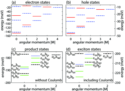
Figure 2: (Color online) Energy-level structure in dependence of angular momentum $M$ in the absence of an external electric field. (a) Electron states with main localization in lower (red, solid) or upper (blue, dashed) dot. (b) Hole states in the same way. (c) Product states of electron and hole (without Coulomb interaction), classified according to a spatially direct configuration (green, solid) and an indirect configuration with a positive (black, dashed) or negative (blue, dotted) sign of the electric dipole moment. (d) Exciton states (including Coulomb interaction) with the same coding as in (c). The labels in (c) and (d) refer to the main localization of electron (e) and hole (h) in the upper (u) or lower (l) dot as well as the shell ($s,p,d$) of the dominant contribution.

Figure 2 shows the energy levels of the confined electron (a), hole (b), product (c) and exciton (d) states. Electrons and holes exhibit essentially the same structure, but the absolute values and separations of the hole energies are much smaller because of the weaker confinement and the larger mass. For the chosen geometry of the QDM, the lowest state of both carriers is mainly localized in the lower dot (red, solid lines), which is, in terms of the standard terminology, of an $s$-shell like character. This state is closely followed by another $s$-shell like state localized in the upper dot (blue, dashed lines). This sequence is caused by the larger height of the lower dot. The energetically next higher state of each dot has an angular momentum of one ($p$-shell). Due to the cylindrical symmetry of the system, the $p$-shells of each dot consist of two degenerate states with $M=\pm 1$. For the $p$-shells, as for all subsequent shells, the lowest state is localized in the upper dot. The order in energy is inverted compared to the $s$-shell because the base radius of the upper dot is larger than the radius of the lower dot. Hence, the almost equidistant sequence of shells of the upper dot is more compact than for the lower dot. For a $d$-shell state we have to distinguish between an angular momentum of two and zero. These states are not degenerate, as we do not have a harmonic confinement (for the hole: $E_{M=0}-E_{M=2}\approx 1\leavevmode\nobreak\$meV). In the following, we denote the single-particle states by their main localization (u for upper and l for lower dot) and their basic type ($s$-, $p$-, $d$-…shell like state), e.g., e${}_{\text{l}s}$ for an electron $s$-shell state in the lower dot.

From the electron and hole single-particle states pair states (excitons) can be formed. For such pair states in a QDM, one has to distinguish between a spatially direct and a spatially indirect configuration. The electron and the hole of a direct exciton are mainly localized in the same dot. The behavior of such an exciton is similar to an exciton in a single QD. In case of an indirect configuration, the electron and the hole are mainly localized in different dots. Therefore, even without an applied electric field the indirect exciton has an electric dipole moment p, roughly proportional to $\pm e\,D$. Thus its energy shifts linearly with an external electric field F. Because the overlap of the electron and hole wave functions is negligible, indirect excitons are not optically active. However, they can become visible in an absorption spectrum due to state mixing with bright, direct excitons, if the coupling between these two configuration is allowed.

In Fig. 2(c) we have plotted a section of the energy structure of the product states of electron and hole ($\tilde{\Psi}_{ij}$, neglecting Coulomb interaction). The states are distinguished according to a direct configuration (green, solid lines), an indirect configuration with a positive dipole moment (black, dashed lines), and an indirect configuration with a negative dipole moment (blue, dotted lines).

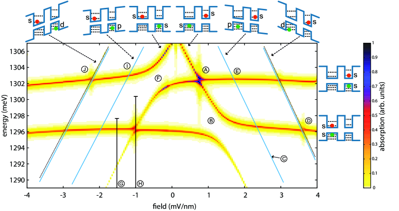
Figure 3: (Color online) Absorption spectrum as a function of the applied electric field at a temperature of $T=10$ K with schemes of the involved exciton states. In the schemes the right potential well refers to the upper dot and the left well to the lower dot. The labels refer to the spectral features and positions discussed in the text. Vertical bars at \textsf{{\scriptsize{G}}}⃝ and \textsf{{\scriptsize{H}}}⃝ indicate the spectral range shown in Fig. 6.

Figure 2(d) shows the energies of the exciton states including Coulomb interaction, as obtained from the diagonalization of the Hamiltonian in Eq. (6). The coding of the lines is the same as in part (c). Although an exciton state is a superposition of electron-hole product states according to Eq. (7), there is in many cases a dominant electron- and hole-contribution, which we use to label the exciton state, e.g., as e${}_{{\text{l}s}}$h${}_{{\text{u}p}}$. In the absence of Coulomb coupling, the lowest indirect states, e${}_{{\text{u}s}}$h${}_{{\text{l}s}}$ and e${}_{{\text{l}s}}$h${}_{{\text{u}s}}$, are lower in energy than the second direct state e${}_{{\text{u}s}}$h${}_{{\text{u}s}}$. This is reversed by taking Coulomb interaction into account, because of the much stronger attraction of electron and hole for a direct exciton. Besides these localization-dependent energy shifts, Coulomb interaction couples different product states, which is important to understand some phenomena of the absorption spectra in the next section.

III.2 Absorption spectra

Figure 3 shows a contour plot of the absorption spectrum of the QDM as a function of the photon energy $E$ and the electric field $F$, which is applied opposite to the growth direction, i.e., a positive value of $F$ refers to a positively charged top contact. The spectral widths of the lines caused by the interaction with phonons can be extracted from the color coding.

The horizontal line at 1.296 eV corresponds to the lowest direct exciton state localized in the lower dot, e${}_{{\text{l}s}}$h${}_{{\text{l}s}}$, while the line at 1.302 eV corresponds to the direct exciton in the upper dot, e${}_{{\text{u}s}}$h${}_{{\text{u}s}}$. For the given values of QD heights and applied fields, the quantum confined Stark effect (QCSE) is only slightly visible by the slight curvature of the absorption lines of the direct excitons with a maximum at zero field. The horizontal lines are intersected by lines corresponding to indirect exciton states, the energy of which shifts linearly with the applied field due to the linear Stark effect $E_{\text{Stark}}\propto-\textbf{p}\cdot\textbf{F}\approx\pm eDF$. Hence, for increasing electric fields $F$, indirect-exciton states with the hole mainly localized in the lower dot and the electron mainly localized in the upper dot [blue, dotted states in Fig. 2(d)] shift downward in energy, while those with the opposite localization of electron and hole [black, dashed states in Fig. 2(d)] shift upward in energy. The former states have the following sequence in energy: e${}_{{\text{u}s}}$h${}_{{\text{l}s}}$, e${}_{{\text{u}s}}$h${}_{{\text{l}p}}$, e${}_{{\text{u}s}}$h${}_{{\text{l}d}}$, e${}_{{\text{u}s}}$h${}_{{\text{l}f}}$, e${}_{{\text{u}p}}$h${}_{{\text{l}s}}$, …while the latter have the same sequence with lower and upper dot exchanged. This order holds for a wide range of parameters, while the distance in energy depends on the specific choice of parameters, like the ratio of carrier masses or strengths of confinement potentials.

As is evident from Fig. 3, at some of the intersections between direct and indirect excitons the energy levels just cross without being visible in the absorption spectrum while at other points a more or less pronounced avoided crossing appears in the spectrum. At \textsf{{\scriptsize{A}}}⃝ we observe such an avoided crossing of the direct state e${}_{{\text{u}s}}$h${}_{{\text{u}s}}$ and the indirect state e${}_{{\text{u}s}}$h${}_{{\text{l}s}}$. Here the hole states in the two dots mix due to tunnel coupling which makes both excitons optically bright in the mixing region. An even more pronounced avoided crossing of e${}_{{\text{l}s}}$h${}_{{\text{l}s}}$ and e${}_{{\text{u}s}}$h${}_{{\text{l}s}}$ appears at \textsf{{\scriptsize{B}}}⃝, which is induced by the tunnel coupling of the electron states in the two dots. The difference in strength of these avoided crossings stems mainly from the difference of electron and hole masses, which favors electron tunneling.

The indirect exciton with the hole having the character of a $p$-shell state (\textsf{{\scriptsize{C}}}⃝; blue, solid line) runs about 11 meV above the previous indirect-exciton state. Due to conservation of angular momentum this state is dark (dipole-forbidden) and decoupled from the visible direct-exciton states. A straight crossing with both direct states occurs, which however can be changed by SO coupling (cf. Sec. III.4) or a perturbation of the cylindrical symmetry of the system (cf. Sec. III.5).

For an exciton with a hole in the $d$-shell (e${}_{{\text{u}s}}$h${}_{{\text{l}d}}$), there are three different configurations: the dark, decoupled ones with angular momenta $M=\pm 2$ (solid, blue line), and the dipole-allowed configuration with $M=0$ (dotted, black line). The former states are not coupled to the direct state e${}_{{\text{l}s}}$h${}_{{\text{l}s}}$ due to the conservation of angular momentum. But also the latter one is not coupled by tunnel coupling to this direct state because tunneling is a single-particle process, while in these two pair-configurations the states of both particles differ. Hence, in the absence of Coulomb interaction, straight crossings would occur. However, a weak anticrossing at a field of $3.6$ mV/nm, \textsf{{\scriptsize{D}}}⃝, appears between the two states with $M=0$ because of Coulomb interaction. Being a a two-particle interaction, it leads to a coupling between excitons with the same total angular momentum, especially at an exciton resonance, i.e., E(e${}_{{\text{u}s}}$h${}_{{\text{l}d}}$) $\approx$ E(e${}_{{\text{l}s}}$h${}_{{\text{l}s}}$), even if all four involved single-particle states are different. The strict discrimination between the $d$-shell states with $M=0$ and $M=\pm 2$ is a consequence of the cylindrical symmetry, which is why in the case of a broken symmetry the anticrossing structure becomes more complicated (cf. Sec. III.5).

The next two indirect states (e${}_{{\text{u}s}}$h${}_{{\text{l}f}}$ and e${}_{{\text{u}p}}$h${}_{{\text{l}s}}$) have a nonzero angular momentum. They have no dipole-allowed transitions and are decoupled from the direct states with angular momentum $M=0$, and are therefore not depicted.

For negative fields the indirect states with a negative dipole moment shift up in energy, while the indirect states with the hole mainly localized in the upper dot (black, dashed lines in Fig. 2(d)) shift down. Hence, the upper anticrossing at $-0.5$ mV/nm (\textsf{{\scriptsize{F}}}⃝) is caused by the tunnel coupling of the electron in e${}_{{\text{u}s}}$h${}_{{\text{u}s}}$ and e${}_{{\text{l}s}}$h${}_{{\text{u}s}}$, instead of the hole-tunnel coupling for positive fields at \textsf{{\scriptsize{A}}}⃝ with e${}_{{\text{u}s}}$h${}_{{\text{l}s}}$. Basically the sequence of crossings and anticrossings of upper and lower dot swaps with the sign of the applied field (\textsf{{\scriptsize{F}}}⃝ corresponds to \textsf{{\scriptsize{B}}}⃝, \textsf{{\scriptsize{J}}}⃝ corresponds to \textsf{{\scriptsize{D}}}⃝ and so on). In this case however, the distances in field strength between the crossings and anticrossings are smaller due to the smaller energy distance of the upper dot’s states. This sequence of crossings and anticrossings is similar to the case of positive field strengths but with upper and lower dots interchanged (although minor differences occur, as the QDM is not symmetric with respect to the growth axis).

III.3 Phonon-mediated transitions

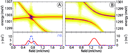
Figure 4: (Color online) Absorption spectrum as a function of the applied electric field (top) and phonon-mediated transition rates from the upper to the lower state (bottom) due to piezoelectric coupling (blue, dashed) and deformation potential (red, solid) at 10 K. In the left panel the rate for piezoelectric coupling has been scaled down by a factor of $1/10$. Left: Hole-anticrossing \textsf{{\scriptsize{A}}}⃝. Right: Electron-anticrossing \textsf{{\scriptsize{B}}}⃝.

In Fig. 3 the width of the absorption lines caused by the interaction with acoustic phonons has already been indicated by the color coding. We will now discuss these line widths in some more detail. In the upper panels of Fig. 4 the absorption spectra in the region of the anticrossings caused by the tunnel-coupling of the holes (\textsf{{\scriptsize{A}}}⃝, left figure) and of the electrons (\textsf{{\scriptsize{B}}}⃝, right figure) are plotted again as functions of the electric field. The lower panels show the corresponding rate $\gamma$ for a transition from the upper to the lower state by phonon emission due to DP (red, solid) and PE coupling (blue, dashed). Note that the rate for PE coupling has been scaled down by a factor of $1/10$. Only in the regions of the anticrossings there is a considerable overlap of the exciton states on the different branches, such that phonon-assisted transitions can take place. In the case of the hole-anticrossing, which is characterized by a weak splitting, we find a large transition rate of the order of 100 ns^-1 corresponding to a lifetime of the upper state of about 10 ps due to the piezoelectric coupling (blue, dashed line). This short lifetime is in good agreement with recent experimental observations.Müller et al. (2012) The PE coupling is strong only in a small energy window of about $0.3-0.9$ meV, where it strongly dominates over the DP coupling. DP coupling is typically strongest for energy differences in the range of $1-2$ meV. Therefore the maxima of the transition rate due to DP interaction in the case of the hole anticrossing appear on both sides of the anticrossing. For the electron anticrossing, the PE coupling is unimportant because of the large energy difference of the states. Here the rate due to DP coupling has its maximum at the center of the anticrossing. In both cases the rate reaches at most a value of about 10 ns^-1 corresponding to a lifetime of about 100 ps. In a QDM there is an oscillatory contribution to the transition rate, which is a typical behavior for quasi one-dimensional phonon scattering;Bockelmann and Bastard (1990); Gawarecki et al. (2010); Wijesundara et al. (2011); Rolon et al. (2012) it is a result of a resonance condition between the phonon wavelength and the distance between the dots. This is the origin of the weak revivals on both sides of the maximum.

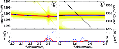
Figure 5: (Color online) Absorption spectrum as a function of the applied electric field (top) and phonon-mediated transition rates from the upper to the lower state (bottom) due to piezoelectric coupling (blue, dashed) and deformation potential (red, solid) at 10 K. In the left panel the rate for piezoelectric coupling has been scaled down by a factor of $1/10$. Left: Coulomb-anticrossing at \textsf{{\scriptsize{D}}}⃝. Right: Crossing of exciton states with different angular momenta at \textsf{{\scriptsize{E}}}⃝.

Figure 5 shows in the same way the spectra in the region of the Coulomb-induced exciton-anticrossing (\textsf{{\scriptsize{D}}}⃝, left figure) and of a crossing (\textsf{{\scriptsize{E}}}⃝, right figure) of exciton states with different angular momenta of $M=0$ (horizontal) and $|M|=1$ (dashed line). The strength of the Coulomb anticrossing as well as the rates of the phonon-mediated transitions are similar to the case of the hole-anticrossing in Fig. 4 (left). This illustrates that the exciton transitions due to phonons do not depend on the coupling mechanism between the involved states. They just depend on the energy separation and the spatial overlap of the states. In the case of crossing exciton states (Fig. 5, right) phonon-assisted transitions are almost absent. The involved states are completely uncoupled due to the conservation of angular momentum and no mixing of the states occur. Since the phonon modes do not have a well-defined angular momentum there is a slight coupling resulting from the weak overlap of the wave functions, however the rate remains very small.

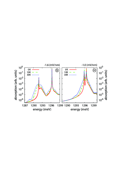
Figure 6: (Color online) Line shape of the absorption spectra for different temperatures at two values of the static electric field: At the hole tunnel-anticrossing \textsf{{\scriptsize{H}}}⃝ (-1 mV/nm) and at a lower field of -1.5 mV/nm \textsf{{\scriptsize{G}}}⃝.

The shape of an absorption line depends crucially on the phonon environment and therefore on temperature.Besombes et al. (2001); Borri et al. (2001, 2003) This is illustrated in Fig. 6 where absorption spectra for two fixed electric fields are shown: At the hole tunnel-anticrossing (\textsf{{\scriptsize{H}}}⃝, right figure) and at a lower electric field on the same direct exciton line (\textsf{{\scriptsize{G}}}⃝, left figure). In each figure, two pronounced peaks (ZPLs) with a temperature dependent background (sidebands) stemming from the states e${}_{{\text{l}s}}$h${}_{{\text{l}s}}$ and e${}_{{\text{l}s}}$h${}_{{\text{u}s}}$ are visible. This shape is characteristic for pure dephasing in QDs. The central peaks are of Lorentzian shape with a broadening that reflects the lifetime of the given state ($\tau_{n}$) with respect to real transitions (relaxation processes). At low temperatures, where no phonon absorption processes are possible, the width of the lowest ZPL is determined by the background lifetime. Outside of the anticrossing region (left figure) there are no phonon-assisted transitions from the upper state, either, because of the lack of final states in the phonon-coupled range. Hence, also the width of the ZPL of the upper line is limited by the background lifetime. At the anticrossing (right figure), on the other hand, the upper line exhibits a pronounced additional broadening, because here phonon-mediated relaxation to the lower branch is more possible. The sidebands are related to the phonon-assisted absorption of light. For zero temperatures, only phonon emission can accompany a photon absorption, so that the sideband appears only at the high energy side of the ZPL. With increasing temperature, a sideband appears also on the low-energy side and grows until the sidebands become symmetric at sufficiently high temperature. Slight modulations of the sidebands again reflect the resonances resulting from the interplay between phonon wavelength and QD separation.

III.4 Spin-Orbit Coupling

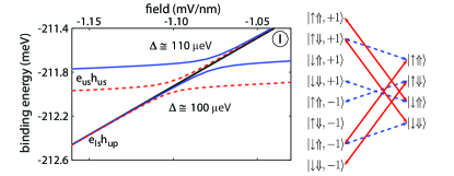
Figure 7: (Color online) Left: Binding energies of the exciton states e${}_{{\text{u}s}}$h${}_{{\text{u}s}}$ and e${}_{{\text{l}s}}$h${}_{{\text{u}p}}$ as a function of the applied field, including different spin configurations and spin-orbit interaction. Right: Scheme of the coupling of the states at the anticrossing due to SOC of electron (red, solid lines) and hole (blue, dashed lines).

For the previous discussions we assumed strict conservation of angular momentum as a consequence of the cylindrical symmetry of the structure. Therefore excitons with different values of the angular momentum did not couple. This conservation is broken by spin-orbit coupling (SOC), although its effects are typically small. For the crossing of the states e${}_{{\text{u}s}}$h${}_{{\text{u}s}}$ and e${}_{{\text{l}s}}$h${}_{{\text{u}p}}$ around $-1$ mV/nm, \textsf{{\scriptsize{I}}}⃝ in Fig. 3, we will now include SOC in the calculations as described in section II.4. Figure 7 (left) shows the corresponding exciton energies as a function of the applied field. The direct exciton splits up in two bright ($\left|\uparrow\Downarrow\right\rangle$ and $\left|\downarrow\Uparrow\right\rangle$) and two dark ($\left|\uparrow\Uparrow\right\rangle$ and $\left|\downarrow\Downarrow\right\rangle$) spin configurations, where the latter two are shifted downward by $0.2\leavevmode\nobreak\$meV due to the exchange interaction. For the indirect exciton we have to consider additionally two different hole orbital-states with angular momentum of $\pm 1$, adding up to eight states (Fig. 7, right). The indirect-exciton states with $\left|\downarrow\Uparrow,+1\right\rangle$ and $\left|\uparrow\Downarrow,-1\right\rangle$ are not coupled by SOC to the direct-exciton states and remain unaffected (black line). The remaining states can be grouped into three subsets of coupled states: $\left|\uparrow\Uparrow,+1\right\rangle,\left|\downarrow\Uparrow\right\rangle,\left|\downarrow\Downarrow,+1\right\rangle$ and $\left|\uparrow\Uparrow,-1\right\rangle,\left|\uparrow\Downarrow\right\rangle,\left|\downarrow\Downarrow,-1\right\rangle$, where the $s$-state is coupled to the $p$-states by hole or electron SOC (note that the $p$-state has contributions of the single-particle $p$-state of hole and electron because of Coulomb interaction). The coupling of these states gives rise to the upper anticrossing (blue, solid lines). In the last subspace with $\left|\uparrow\Uparrow\right\rangle,\left|\downarrow\Uparrow,-1\right\rangle,\left|\uparrow\Downarrow,+1\right\rangle$ and $\left|\downarrow\Downarrow\right\rangle$, the dark, direct states are indirectly coupled to each other. This results in the lower anticrossing (red, dashed lines) with an energy separation of about 100 $\mu$eV. The effect of SOC vanishes quickly out of resonance. Although the mixing of the states supports phonon-mediated transitions, the effect is very small, as the splitting remains in an energy range with a very low spectral density $J_{nm}(\omega_{nm})$.

III.5 Confinement potentials with broken cylindrical symmetry

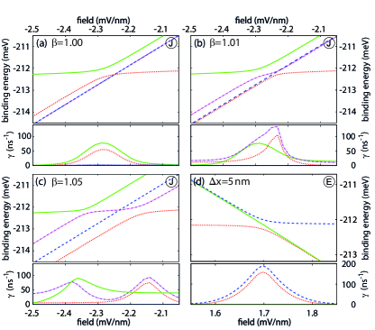
Figure 8: (Color online) Exciton binding energies (top) and phonon-mediated transition rates (DP+PE, at 10 K) (bottom), as a function of the applied field for cases with broken cylindrical symmetry. (a)-(c): Elliptical dots at \textsf{{\scriptsize{J}}}⃝. (d): QDs displaced by $5\leavevmode\nobreak\$nm at \textsf{{\scriptsize{E}}}⃝. Transition rates shown in the bottom panels refer to the states represented by the same line style.

So far, we have considered a structure with cylindrical symmetry, such that – in the absence of SOC – angular momentum has been a good quantum number. In a real structure the cylindrical symmetry of the confining potentials can be broken, e.g., if one or both QDs exhibit elliptical elongations in a specific direction, or in the case of an imperfect alignment, i.e., a lateral displacement of the center of the two QDs. Such structures with a broken cylindrical symmetry are described by an additional contribution $H_{\mathrm{bs}}^{\mathrm{e/h}}$ to the confinement potentials of electrons and holes. Here we will analyze the role of these types of symmetry breaking for the coupling between different direct and indirect excitons. We will assume that the deviations from cylindrical symmetry are not too strong such that they can be treated in a perturbative way.

In the case of an elliptical deformation of the confinement potentials degeneracies are removed, e.g., the p-shell splits into $p_{x}$ and $p_{y}$. Between these states phonon-assisted transitions can become rather efficient. However, a two-fold rotational symmetry axis is still present and no coupling between $p$- and $s$-state emerges. On the level of the present envelope function formalism, this selection rule can only be broken if the dot symmetry is reduced even further, which seems rather unusual.

For a dot with a harmonic in-plane confinement, ellipticity can be described by a difference in the potentials of $x$- and $y$-direction, i.e., $\omega_{x}\neq\omega_{y}$. Assuming the same deviation from cylindrical symmetry of both dots, this ellipticity is described in polar coordinates ($\rho,\phi$) by the Hamiltonian

$$H_{\mathrm{bs}}^{\mathrm{e/h}}=H_{\mathrm{ellip.}}^{\mathrm{e/h}}=\frac{1}{2}m_{\mathrm{e/h}}\bar{\omega}_{\mathrm{e/h}}^{2}\rho^{2}\frac{\beta^{4}-1}{\beta^{4}+1}\cos(2\phi),$$ (28)

where $\bar{\omega}_{\mathrm{e/h}}^{2}=[(\omega^{\mathrm{e/h}}_{\textrm{u}})^{2}+(\omega^{\mathrm{e/h}}_{\textrm{l}})^{2}]/2$ is an average of the confinement frequencies of the upper and lower dot, and $\beta=\sqrt{\omega^{\mathrm{e/h}}_{x}/\omega^{\mathrm{e/h}}_{y}}$ describes the ratio of the $x$- and $y$-axes of the ellipse. We will use the same form as an effective additional potential and extract the confinement frequencies $\omega^{\mathrm{e/h}}_{\textrm{u/l}}$ of upper and lower dot from the splitting between $s$- and $p$-shell states of electrons and holes in the upper and lower dot, respectively. The asymmetry parameter $\beta$ is taken to be the same for electrons and holes. Equation (28) indicates that the perturbation vanishes between all states $i,j$ with $M_{i}-M_{j}\neq\pm 2$.

In the case of a lateral mismatch of the dots, the strict separation of states with different in-plane parity is broken. For a harmonic confinement potential a relative displacement by $\Delta x$ of the upper dot with respect to the lower dot can be introduced by the perturbation

$$H_{\mathrm{bs}}^{\mathrm{e/h}}=H_{\text{displ.}}^{\mathrm{e/h}}=m_{\mathrm{e/h}}(\omega_{\textrm{u}}^{\mathrm{e/h}})^{2}\left(\frac{\Delta x^{2}(z)}{2}-\Delta x(z)\,\rho\,\cos(\phi)\right)$$ (29)

with

$$\Delta x(z)=\frac{\Delta x}{2}\left[\tanh\left(\frac{z-z_{0}}{a}\right)+1\right],$$

where the $\tanh$-function ensures a smooth transition of the potential between the dots, $z_{0}$ is the $z$-coordinate in the middle between both dots, and $a$ is a parameter that controls the smoothing, which we take to be 1 nm. Evidently, this perturbation gives rise to a coupling between states with $M_{i}-M_{j}=\pm 1$.

For both types of symmetry-breaking potentials we calculate the matrix elements in the truncated basis of the single particle states, which leads to an additional contribution

$$\sum_{ij}\left(H_{\mathrm{bs}}^{\mathrm{e}}\right)_{ij}c^{\dagger}_{i}c^{\phantom{\dagger}}_{j}+\sum_{ij}\left(H_{\mathrm{bs}}^{\mathrm{h}}\right)_{ij}d^{\dagger}_{i}d^{\phantom{\dagger}}_{j}$$ (30)

to the interacting particle Hamiltonian in Eq. (4). From this extended Hamiltonian the modified exciton energies and wave functions are then obtained by numerical diagonalization within the basis of electron-hole pair states.

Figures 8(a)-(c) show the exciton energy of the shells e${}_{{\text{u}s}}$h${}_{{\text{u}s}}$ and e${}_{{\text{l}s}}$h${}_{{\text{u}d}}$ as a function of the applied field for different elongations around \textsf{{\scriptsize{J}}}⃝ in Fig. 3. For a symmetric dot, i.e., $\beta=1.00$ [Fig. 8(a)], the degenerate $d$-states with $M=\pm 2$ (blue, dashed line) are uncoupled from the horizontal $s$-state and the other $d$-state with $M=0$, which run through an avoided crossing (red, dotted and green, solid lines). In the presence of an ellipticity ($\beta\neq 1$) the states with $M=\pm 2$ mix leading to the symmetry-adapted states with angular dependencies $\sim\cos(2\phi)$ and $\sim\sin(2\phi)$. By means of the Hamiltonian in Eq. (28) the former state now is coupled to $s$-states as well as to $d$-states with $M=0$ while the latter state remains uncoupled. This is indeed seen in Figs. 8(b),(c) where we observe the lifting of the degeneracy of the two $d$-states and the appearance of a new anticrossing while the blue, dashed line, corresponding to the state with the sine-like angular dependence, still exhibits a crossing behavior. For a ratio of the dot axes of $\beta=1.01$, the degeneracy of the states is only slightly lifted and a small additional anticrossing emerges. The splitting between the $d$-states, as well as the anticrossing, becomes larger for a stronger ellipticity [$\beta=1.05$ in Fig. 8(c)], while the other anticrossing shrinks.

The lower parts of Figs. 8(a)-(c) show the corresponding phonon-mediated transition rates. The rates are increased at an anticrossing, with the higher state having a larger transition rate because of the relaxation to the lower state. For the coupled $d$-states in Fig. 8(b) and (c) phonon-assisted transitions occur also out of the anticrossing region. This is caused by intrashell transitions within the $d$-shell, which become noticeable for sufficiently large splitting between the $d$-shell states. Hence, they only depend on the ellipticity of the dots and stay at a constant level out of the region of an avoided crossing. Phonon-mediated transitions of the uncoupled $d$-state remain negligible.

Also in the case of a lateral displacement of one of the QDs with respect to the other the angular momentum eigenstates mix to states with a sine- or cosine-like angular dependence. This is seen in Fig. 8(d), where the exciton energies of e${}_{{\text{u}s}}$h${}_{{\text{u}s}}$ and e${}_{{\text{u}s}}$h${}_{{\text{l}p}}$ are depicted in the region around the former crossing between $s$- and $p$-states (\textsf{{\scriptsize{E}}}⃝ in Fig. 3) for the case of a displacement of the upper dot by $\Delta x=5$ nm with respect to the lower dot. An anticrossing with a splitting $\Delta E\approx 300$ $\mu$eV appears due to the coupling between the $p_{x}$-state [$\sim\cos(\phi)$] with the $s$-state, while the $p_{y}$-state [$\sim\sin(\phi)$] is uncoupled. Here, the degeneracy of the $p$-shell is only lifted in an area around the avoided crossing, because out of this region the states are mainly localized in one of the dots and therefore experience only a very weak deviation from cylindrical symmetry.

The lower part of Fig. 8(d) depicts the transition rates of the exciton states. The rates of the coupled exciton states are rather high, since the energy separation at the anticrossing is in the range of an efficient phonon coupling. For the uncoupled state the transition rates remain at a very low level.

IV Conclusion

We have investigated excitons in QDMs, in particular their absorption spectra and the influence of the phonon environment on the spectra. Three different kinds of anticrossings, which are caused by tunnel coupling, Coulomb interaction and spin-orbit coupling, were discussed, as well as the influence of a broken cylindrical symmetry induced, e.g., by an elliptical elongation of the dots or a lateral displacement of the centers of the QDs.

We have found that the ordering of the energies of the states is strongly modified by the Coulomb interaction, compared to the sequence of combined single-particle energies. The Coulomb interaction causes additional anticrossings between exciton states leading to an enhanced phonon relaxation in the regions of such anticrossings, comparable to the situation of a tunnel coupling of the hole. The shape of the absorption lines is characterized by a zero phonon line superimposed on a broad phonon background. The latter one results from the pure daphasing-type part of the exciton-phonon coupling, while the width of the ZPLs can be enhanced by real phonon transitions to other exciton states, which occurs mainly in the region of an anticrossing. The resonance between the phonon wavelength and the separation of the QDs gives rise to characteristic modulations in the phonon scattering rates and the phonon background.

Although the cylindrical symmetry of the confinement potential supports conservation of angular momentum, spin-orbit coupling removes this conservation and leads to more complex anticrossings at an exciton resonance. The energy splitting introduced by this coupling, however, are typically rather small such that no efficient phonon scattering between the states occurs.

In the case of a perturbation of the cylindrical symmetry of the confinement potential, we have found that an elliptical elongation leads to additional avoided crossings near resonances between states with angular momenta differing by two and thus to energy splittings of otherwise degenerate states. In contrast, a displacement of the center of the dots provides an additional mixing of otherwise uncoupled states for any difference of the angular momenta.

Acknowledgements

This work was supported in part by a Research Group Linkage Project of the Alexander von Humboldt Foundation and by the TEAM programme of the Foundation for Polish Science, co-financed by the European Regional Development Fund. Fruitful discussions with Jonathan Finley, Kai Müller, and Krzysztof Gawarecki are gratefully acknowledged.

References

- Bayer et al. (2001) M. Bayer, P. Hawrylak, K. Hinzer, S. Fafard, M. Korkusinski, Z. R. Wasilewski, O. Stern, and A. Forchel, Science, 291, 451 (2001).
- Krenner et al. (2005) H. J. Krenner, M. Sabathil, E. C. Clark, A. Kress, D. Schuh, M. Bichler, G. Abstreiter, and J. J. Finley, Phys. Rev. Lett., 94, 057402 (2005).
- Stinaff et al. (2006) E. A. Stinaff, M. Scheibner, A. S. Bracker, I. V. Ponomarev, V. L. Korenev, M. E. Ware, M. F. Doty, T. L. Reinecke, and D. Gammon, Science, 311, 636 (2006).
- Bracker et al. (2006) A. S. Bracker, M. Scheibner, M. F. Doty, E. A. Stinaff, I. V. Ponomarev, J. C. Kim, L. J. Whitman, T. L. Reinecke, and D. Gammon, Appl. Phys. Lett., 89, 233110 (2006).
- Robledo et al. (2008) L. Robledo, J. Elzerman, G. Jundt, M. Atatüre, A. Högele, S. Fält, and A. Imamoglu, Science, 320, 772 (2008).
- Goryca et al. (2009) M. Goryca, T. Kazimierczuk, M. Nawrocki, A. Golnik, J. A. Gaj, P. Kossacki, P. Wojnar, and G. Karczewski, Phys. Rev. Lett., 103, 087401 (2009).
- Shulman et al. (2012) M. D. Shulman, O. Dial, S. P. Harvey, H. Bluhm, V. Uhmansky, and A. Yacoby, Science, 366, 202 (2012).
- Bester et al. (2004) G. Bester, J. Shumway, and A. Zunger, Phys. Rev. Lett., 93, 047401 (2004).
- Schliwa et al. (2001) A. Schliwa, O. Stier, R. Heitz, M. Grundmann, and D. Bimberg, Phys. Status Solidi B, 224, 405 (2001).
- Szafran et al. (2005) B. Szafran, T. Chwiej, F. M. Peeters, S. Bednarek, J. Adamowski, and B. Partoens, Phys. Rev. B, 71, 205316 (2005).
- Szafran (2008) B. Szafran, Acta Phys. Pol. A, 114, 1013 (2008).
- Gawarecki et al. (2010) K. Gawarecki, M. Pochwała, A. Grodecka-Grad, and P. Machnikowski, Phys. Rev. B, 81, 245312 (2010).
- Bryant (1993) G. W. Bryant, Phys. Rev. B, 47, 1683 (1993).
- Scheibner et al. (2008) M. Scheibner, M. Yakes, A. S. Bracker, I. V. Ponomarev, M. F. Doty, C. S. Hellberg, L. J. Whitman, T. L. Reinecke, and D. Gammon, Nat. Phys., 4, 291 (2008).
- Ortner et al. (2005) G. Ortner, M. Bayer, Y. Lyanda-Geller, T. L. Reinecke, A. Kress, J. P. Reithmaier, and A. Forchel, Phys. Rev. Lett., 94, 157401 (2005a).
- Ortner et al. (2003) G. Ortner, M. Bayer, A. Larionov, V. B. Timofeev, A. Forchel, Y. B. Lyanda-Geller, T. L. Reinecke, P. Hawrylak, S. Fafard, and Z. Wasilewski, Phys. Rev. Lett., 90, 086404 (2003).
- Lyanda-Geller et al. (2004) Y. B. Lyanda-Geller, T. L. Reinecke, and M. Bayer, Phys. Rev. B, 69, 161308 (2004).
- Ortner et al. (2005) G. Ortner, I. Yugova, G. Baldassarri Höger von Högersthal, A. Larionov, H. Kurtze, D. R. Yakovlev, M. Bayer, S. Fafard, Z. Wasilewski, P. Hawrylak, Y. B. Lyanda-Geller, T. L. Reinecke, A. Babinski, M. Potemski, V. B. Timofeev, and A. Forchel, Phys. Rev. B, 71, 125335 (2005b).
- Müller et al. (2011) K. Müller, G. Reithmaier, E. C. Clark, V. Jovanov, M. Bichler, H. J. Krenner, M. Betz, G. Abstreiter, and J. J. Finley, Phys. Rev. B, 84, 081302 (2011).
- Heldmaier et al. (2012) M. Heldmaier, M. Seible, C. Hermannstädter, M. Witzany, R. Roßbach, M. Jetter, P. Michler, L. Wang, A. Rastelli, and O. G. Schmidt, Phys. Rev. B, 85, 115304 (2012).
- Takagahara (1999) T. Takagahara, Phys. Rev. B, 60, 2638 (1999).
- Krummheuer et al. (2002) B. Krummheuer, V. M. Axt, and T. Kuhn, Phys. Rev. B, 65, 195313 (2002).
- Borri et al. (2003) P. Borri, W. Langbein, U. Woggon, M. Schwab, M. Bayer, S. Fafard, Z. Wasilewski, and P. Hawrylak, Phys. Rev. Lett., 91, 267401 (2003).
- Stavrou and Hu (2005) V. N. Stavrou and X. Hu, Phys. Rev. B, 72, 075362 (2005).
- Benisty (1995) H. Benisty, Phys. Rev. B, 51, 13281 (1995).
- Besombes et al. (2001) L. Besombes, K. Kheng, L. Marsal, and H. Mariette, Phys. Rev. B, 63, 155307 (2001).
- López-Richard et al. (2005) V. López-Richard, S. S. Oliveira, and G. Q. Hai, Phys. Rev. B, 71, 075329 (2005).
- Vorojtsov et al. (2005) S. Vorojtsov, E. R. Mucciolo, and H. U. Baranger, Phys. Rev. B, 71, 205322 (2005).
- Wu et al. (2005) Z.-J. Wu, K.-D. Zhu, X.-Z. Yuan, Y.-W. Jiang, and H. Zheng, Phys. Rev. B, 71, 205323 (2005).
- Grodecka et al. (2008) A. Grodecka, P. Machnikowski, and J. Förstner, Phys. Rev. B, 78, 085302 (2008).
- Gawarecki and Machnikowski (2012) K. Gawarecki and P. Machnikowski, Phys. Rev. B, 85, 041305 (2012).
- Müller et al. (2012) K. Müller, A. Bechtold, C. Ruppert, M. Zecherle, G. Reithmaier, M. Bichler, H. J. Krenner, G. Abstreiter, A. W. Holleitner, J. M. Villas-Boas, M. Betz, and J. J. Finley, Phys. Rev. Lett., 108, 197402 (2012).
- Wijesundara et al. (2011) K. C. Wijesundara, J. E. Rolon, S. E. Ulloa, A. S. Bracker, D. Gammon, and E. A. Stinaff, Phys. Rev. B, 84, 081404 (2011).
- Rolon et al. (2012) J. E. Rolon, K. C. Wijesundara, S. E. Ulloa, A. S. Bracker, D. Gammon, and E. A. Stinaff, J. Opt. Soc. Am. B, 29, A146 (2012).
- Szafran et al. (2001) B. Szafran, S. Bednarek, and J. Adamowski, Phys. Rev. B, 64, 125301 (2001).
- Sheng and Leburton (2002) W. Sheng and J.-P. Leburton, Phys. Rev. Lett., 88, 167401 (2002).
- Janssens et al. (2002) K. L. Janssens, B. Partoens, and F. M. Peeters, Phys. Rev. B, 65, 233301 (2002).
- Szafran et al. (2007) B. Szafran, F. M. Peeters, and S. Bednarek, Phys. Rev. B, 75, 115303 (2007).
- Stano and Fabian (2005) P. Stano and J. Fabian, Phys. Rev. B, 72, 155410 (2005).
- Muljarov et al. (2005) E. A. Muljarov, T. Takagahara, and R. Zimmermann, Phys. Rev. Lett., 95, 177405 (2005).
- Wojs et al. (1996) A. Wojs, P. Hawrylak, S. Fafard, and L. Jacak, Phys. Rev. B, 54, 5604 (1996).
- note (2013) A spatially dependent strain distribution is not taken into account explicitly in the calculations since this is expected to be of minor importance due to the rather low indium content. However, the values for the electron and hole masses are adjusted to reproduce the experimental results from Ref. 32 and therefore the overall effect of strain is included .
- Rossi and Kuhn (2002) F. Rossi and T. Kuhn, Rev. Mod. Phys., 74, 895 (2002).
- Binder et al. (1994) E. Binder, T. Kuhn, and G. Mahler, Phys. Rev. B, 50, 18319 (1994).
- Fox (2001) M. Fox, Optical Properties of Solids, Oxford Master Series in Cendensed Matter Physics I (Oxford University Press, Oxford, 2001).
- Suna (1964) A. Suna, Phys. Rev., 135, A111 (1964).
- Jacak et al. (2005) L. Jacak, J. Krasnyj, W. Jacak, R. Gonczarek, and P. Machnikowski, Phys. Rev. B, 72, 245309 (2005a).
- Jacak et al. (2005) L. Jacak, P. Machnikowski, and J. Krasnyj, “Fast control of quantum states in quantum dots: Limits due to decoherence,” in Quantum Dots: Fundamentals, Applications, and Frontiers, NATO Science Series, Vol. 190, edited by B. A. Joyce, P. C. Kelires, A. G. Naumovets, and D. D. Vvedensky (Springer Netherlands, 2005) Chap. 20, p. 301.
- Dresselhaus (1955) G. Dresselhaus, Phys. Rev., 100, 580 (1955).
- Winkler (2003) R. Winkler, Springer Tracts in Modern Physics Vol. 191: Spin-Orbit Coupling Effects in Two-Dimensional Electron and Hole Systems (Springer, Berlin, 2003).
- Bayer et al. (2002) M. Bayer, G. Ortner, O. Stern, A. Kuther, A. A. Gorbunov, A. Forchel, P. Hawrylak, S. Fafard, K. Hinzer, T. L. Reinecke, S. N. Walck, J. P. Reithmaier, F. Klopf, and F. Schäfer, Phys. Rev. B, 65, 195315 (2002).
- Seguin et al. (2005) R. Seguin, A. Schliwa, S. Rodt, K. Pötschke, U. W. Pohl, and D. Bimberg, Phys. Rev. Lett., 95, 257402 (2005).
- Bockelmann and Bastard (1990) U. Bockelmann and G. Bastard, Phys. Rev. B, 42, 8947 (1990).
- Borri et al. (2001) P. Borri, W. Langbein, S. Schneider, U. Woggon, R. L. Sellin, D. Ouyang, and D. Bimberg, Phys. Rev. Lett., 87, 157401 (2001).