Efficient binary tomographic reconstruction

Abstract

Tomographic reconstruction of a binary image from few projections is considered. A novel heuristic algorithm is proposed, the central element of which is a nonlinear transformation $\psi(p)=\log(p/(1-p))$ of the probability $p$ that a pixel of the sought image be 1-valued. It consists of backprojections based on $\psi(p)$ and iterative corrections. Application of this algorithm to a series of artificial test cases leads to exact binary reconstructions, (i.e., recovery of the binary image for each single pixel) from the knowledge of projection data over a few directions. Images up to $10^{6}$ pixels are reconstructed in a few seconds. A series of test cases is performed for comparison with previous methods, showing a better efficiency and reduced computation times.

1 Introduction

Tomographic reconstruction is a mature topic Kak01 ; Gardner06 for which a variety of algorithms is now available from the celebrated Filtered BackProjection (FBP) FBP , including its fast implementation Basu01a ; Basu01b , to various Algebraic Reconstruction Techniques (ART) Herman76 . Numerous extensions have been proposed for enhanced accuracy or speed. ART appears as the method of choice for a small number of projections or noisy data, whereas FBP is superior in terms of computation times.

A specific class of reconstruction problems appears when the image to be reconstructed has only few gray levels (termed discrete reconstruction) or is binary (i.e., its “pixels” are either black or white) Herman99 ; Herman07 . This additional piece of information is extremely valuable and allows dealing with very few projections, provided the image to be reconstructed is sufficiently “simple.”

However, the discrete nature of the image to be reconstructed renders more difficult the recourse to classical reconstruction algorithms. In order to reach acceptable reconstructions (perfect ones are generally out of reach), optimization techniques specific to NP-complete problems (binary reconstruction has been shown to belong to this class of “hard” problems NPComplete ) were considered, namely, Simulated Annealing (SA) Weber06 ; Liao07 or Genetic Optimization (GO) Varga10 have been proposed and shown to be able to capture approximately synthetic phantoms over images of size $N\times N$, with $N\leq 256$ pixels, and a number $M$ of projections in the range from 4 to 10, within a computation time of order of a few hours (even for recent GPU implementations Varga10 ). Smaller $N$ values, say of order 64 pixels, still require a computation time of the order of a few minutes in those references. Such performances rely on the fact that the image contains few connected domains generally with smooth boundaries. One additional difficulty of such methods is their rather slow convergence and sensitivity to the way the algorithm is driven. In addition, there is no guarantee that the algorithm is not trapped in a local minimum.

In such a context, an iterative correction approach seems more appealing, and recent works have led to much more successful results either in terms of quality of the reconstruction and computation cost Batenburg07 ; Batenburg08 . The binary nature of the sought image, although offering severe constraints that are helpful to compensate for the lack of information, suggests that combinatorial type approaches are needed. Thus, the challenge is to conciliate corrections, which naturally use a continuous representation of the image, and the known a priori information on its binary character. Early attempts Censor to interleave classical reconstruction steps, and “binary steering” favoring 0 or 1 for pixel values showed encouraging results, yet $64\times 64$ images could not be exactly reconstructed after 1000 iterations.

The binary nature of the image constitutes by itself an element of simplicity, namely, a single bit of information is needed per pixel. However, additional elements can further simplify the problem of reconstructing the image from a few projections. In particular, the notion of “sparsity” has been shown in the recent years to allow for very efficient restoration of signals (or here images) from few partial measurements or data. Yet, sparsity may have different appearance. At least two categories can be distinguished:
- Type A. If no spatial correlation exists in the image, then sparsity has to rely only on the number of 1-valued pixels. It has been shown in a series of work starting from Ref. Donoho04 on undersampling theory, that a “phase-transition” exists separating solvable problems from unsolvable ones depending on the quantity of available information. In the framework of sparsity based on the density of non-zero pixels only, the order of magnitude of the maximum concentration of non zero pixels (i.e., number of pixels relative to the image size), $p_{c}$, in a $N\times N$ pixel image, based on $M$ projections has been shown by Donoho and Tanner Donoho10a ; Donoho10b to amount to

$$p_{c}\approx\frac{M}{2N\log(N/M)}$$ (1)

It may be convenient to introduce the undersampling ratio, $\delta\equiv N/M$, so that $p_{c}\approx[2\delta\log(\delta)]^{-1}$. To mention an example, for a 1-Mpixel image, $N=1000$, and $M=10$ projections, $p_{c}$ is of the order of $10^{-3}$, or about one non-zero pixel (at most) per line. This threshold is a theoretical level, yet available algorithms Jafarpour allow such problems to be addressed with an effective threshold that is quite close to the theoretical value. Note that for $p>p_{c}$ still a unique binary solution may exist, but there is no guarantee that this solution can be reached through a convex minimization procedure.
- Type B. Spatial correlations may also contribute to the reduction of “complexity” in the image. If all 1-valued pixels are grouped into a few blobs, the information content of the image is reduced and hence an arbitrary proportion of black or white pixels can be dealt with, and still a small number of projections is needed to reconstruct the image. Along this line, Candés et al. CS_Tomo introduced an algorithm to reconstruct an image from a set of projections provided the image consists of a few number of domains, each of which having a uniform gray level. The key to the solution is here again a low level of “complexity” in the image. However, in contrast with the previous case, spatial correlations are here essential. In this case, the image gradient is a sparse field, and a regularization based on the “total variation” is essential to reach the solution. Although recent works Needell13 progress toward solid results on stable and robust image recovery from noisy data based on total variation minimization, yet a proof of a phase transition for type B problems (comparable to that of type A) is not currently available.

In the following, all examples are believed to belong to the second class of problems. However, no practical definition of the relevant measure of “complexity” can be formally derived as above mentioned for Type A. Based on the above result, an attempt to transpose this measure for the studied cases is provided in Sect. 7. Let us also note that Gouillart et al. Gouillart have recently proposed a different type of algorithm based on “message passing” for binary and discrete tomography reconstruction where it was suggested that the proportion of 0-1 pixel pairs (or interfaces) is responsible for the image “complexity”. The proposed algorithm is essentially heuristic, and no guarantee for convergence is proposed. When too few projections are given, the algorithm does not converge and the residual difference with the sought image fluctuates around a constant value which may not be small. However, when applied to test images which have been proposed earlier Batenburg07 , the reconstruction performance appears as superior both in terms of quality and time.

In terms of applications, many different fields are concerned. Medical imaging is one of the most demanding applications Medical ; Medical1 , and here the interest lies in the X-ray dose reduction for the patient, provided the reconstruction can be limited to two phases. In the field of fluid mechanics, Tomographic Particle Image Velocimetry (Tomo-PIV) reconstruction of tracer particle distribution in a suspending transparent fluid is required from optical images taken by few cameras PIV1 ; PIV2 , hence few projections. Finally, in the field of materials science, an amazing progress has been achieved in the recent years in terms of fast data acquisition FastTomo . Full 3D scans can now be acquired in less than one second in large scale synchrotron facilities. Whenever the microstructure could tolerate a simple representation as a binary image, the reduction in the number of projections could automatically be translated into a larger scanning rate, or finer temporal resolution. These are three examples where progress in the reconstruction using reduced projections would be very rewarding.

Section 2 defines the problem of tomographic reconstruction and presents some regularization strategies classically used in this context. Section 3 introduces the algorithm used, and a first illustration is shown in Section 4. Section 5 introduces a multi-scale formulation that enhances the efficiency of the algorithm. A detailed comparison with some benchmark tests is reported in Section 6. An attempt to rationalize the performances of the text as a function of a proposed measure of complexity is proposed in Sect. 7, and the effect of noise on reconstruction is documented for a single image in Sect. 8. Finally, Section 9 recalls the major results and some perspectives are discussed.

2 Statement of the problem

The problem consists of identifying a binary-valued discrete image $f(\bm{x})$ where $f$ is valued in $\{0,1\}$. $f$ is defined at pixels $\bm{x}$ having integer coordinates, inside a 2D domain, $\bm{x}\in{\cal D}$, chosen in the sequel to be a circular disk of radius $N/2$ where $N$ is an integer. The image is known only from “projections” along a few known directions labeled by $j=1,...,M$. A direction $j$ is characterized by its unit vector $\bm{n}^{j}$, and its $\pi/2$-rotated vector $\bm{t}^{j}$. For each direction $j$, the projection $\pi^{j}(y)$, is defined as the line sum of $f$ along the “ray” that projects onto $y$. This ray is the set of points $\bm{x}$, such that $\bm{x}^{\top}\bm{t}^{j}=y$. The projection is written as

$$\sum_{\bm{x}^{\top}\bm{t}^{j}=y}f(\bm{x})=\pi^{j}(y)$$ (2)

where $|y|\leq N/2$. The $M$ projections $\pi^{j}(y)$ are given and the image $f$ is to be reconstructed.

The total number of pixels is of order $(\pi/4)N^{2}$. In practice it is often more convenient to consider all pixels with the $[-N/2;N/2]^{2}$ square domain that contain the disk $\cal D$. In that case, $i$ ranges from 1 to $N^{2}$, but for those pixels, $\bm{x}_{i}$ which are more distant than $N/2$ from the origin, $f(\bm{x}_{i})=0$. It is convenient to introduce a vector representation of the discrete image through the notation ${\mathbf{f}}=\{f_{i}\}$ where $f_{i}=f(\bm{x}_{i})$. In the sequel, this vector representation will be used systematically, and denoted (as well as matrices) by bold characters.

Let us note that in the literature, the sampling of $\pi^{j}(y)$ is often assumed to be resolved at the scale of the separation between the projection of the discrete pixel centers $\bm{x}_{i}$ (see e.g., Batenburg07 ). For instance, when the projection is performed at $\pi/4$ with respect to the principal axis, pixels are projected onto positions separated by $1/\sqrt{2}$ and hence the number of projection data is $\sqrt{2}N$, as compared to $N$ when the projection direction is 0 or $\pi/2$. As the number of projections, $M$, increases, the size of the discrete vector $\pi^{j}$ increases, so that the information content increases quickly.

For that reason, a different discretization choice is made herein, namely, for any direction, $j$, the $\pi^{j}(y)$ function is binned over intervals of size 1. Introducing equally spaced discrete coordinates $y_{k}$ (with a unit spacing), the projection $\pi^{j}(y)$ is transformed into the series of discrete components

$$\begin{array}[]{ll}\pi^{j}_{k}&\displaystyle=\sum_{|y-y_{k}|<1/2}\pi^{j}(y)\\ &\displaystyle=\sum_{i}H(1/2-|\bm{x}_{i}^{\top}\bm{t}^{j}-y_{k}|)f_{i}\end{array}$$ (3)

where $H$ denotes the Heaviside function, i.e., $H(x)=1$ iff $x\geq 0$, and $H(x)=0$ else. Thus the projection data are collected into $M$ vectors $\bm{\pi}^{j}$ for $1\leq j\leq M$; each vector $\bm{\pi}^{j}=\{\pi^{j}_{k}\}$ being of length $N$, $k=1,...,N$. In that case, any direction brings approximately the same amount of information (i.e., same number $N$ of equations).

For the sake of simplicity, for any projection direction, the choice is made to associate each pixel $\bm{x}_{i}$ with a unique detector site $y_{k}$ onto which the projection is considered (i.e., closest integer value as above defined). It is to be noted that other choices could have been made. In particular, a pixel could be partitioned into different rays with weight corresponding to the area of the square pixel swept by the ray of unit width. The first choice is the simplest as the weight itself is binary. The second is more realistic when considering an actual experiment. In the following only the first choice was made.

In discrete form, these projections are recast in a linear form

$${\mathbf{W}}{\mathbf{f}}={\bm{\pi}}$$ (4)

where the projection operator ${\mathbf{W}}$ is itself a binary matrix as a result of the above projection discretization. This linear system is the collection of the projection equations along different orientations. For a specific direction $\bm{n}^{j}$, this projection operator is denoted by ${\mathbf{W}}^{j}$ and second member ${\bm{\pi}}^{j}$, so that ${W}^{j}_{mn}f_{n}=\pi^{j}_{m}$ where $1\leq j\leq M$, $1\leq m\leq N$ and $1\leq n\leq N^{2}$.

The associated backprojection operator ${\mathbf{B}}^{j}$ is simply deduced from the transpose of ${\mathbf{W}}^{j}$ through a normalization by the number of pixels $N^{j}_{k}$ being projected onto the same detector site. The latter is obtained by the projection ${\mathbf{W}}^{j}\mathbf{1}$ where $1_{n}=1$ for all $1\leq n\leq N^{2}$, $N^{j}_{k}=\sum_{n}W^{j}_{kn}$. Let us introduce the diagonal operator $\mathbf{D}$ such that

$$D^{j}_{kl}=\delta_{kl}/N^{j}_{k}=\delta_{kl}/\sum_{n=1}^{N^{2}}W^{j}_{kn}$$ (5)

where $1\leq j\leq M$, $1\leq k\leq N$, $1\leq l\leq N$, and $\delta_{kl}$ denotes the Kronecker symbol. The backprojection operator is written as

$$B^{j}_{nm}=\frac{W^{j}_{mn}}{\sum_{p=1}^{N^{2}}W^{j}_{mp}}$$ (6)

for $1\leq j\leq M$, $1\leq m\leq N$ and $1\leq n\leq N^{2}$, or equivalently

$${\mathbf{B}}^{j}=(\mathbf{W}^{j})^{\top}{\mathbf{D}}^{j}$$ (7)

so that ${\mathbf{W}}^{j}{\mathbf{B}}^{j}={\mathbf{I}}$.

It is to be emphasized that the number of available equations from the projections is far less than the number of unknowns. Typically for $N=300$ and $M=4$, the ratio of equations over unknown amounts to about 1.5 %, emphasizing the crucial role to be played by the regularization in the solution.

3 Algorithm

Most binary reconstruction methods proposed in the literature, whatever their specific strategy, are iterative. Hence, the first step of any algorithm is to propose a trial image for $f$ to initialize the procedure. The obvious route to follow is to apply the classical fast algorithm known for continuous reconstruction, and hence, typically, it is proposed to start with the standard FBP algorithm from the known projections. Although natural, this procedure is not optimal, and the following subsection aims at revisiting this first step through a more genuine estimate of the local probabilities for a site $i$ to be valued $f_{i}=0$ or 1.

3.1 Initialization

Let us consider a specific site, $\bm{x}_{i}$, and two arbitrary projection directions, 1 and 2. The corresponding projections of $\bm{x}_{i}$ on the detector line are denoted as $k_{1}$ and $k_{2}$ respectively ($W^{1}_{k_{1}i}=1$ and $W^{2}_{k_{2}i}=1$). From the first direction, and without additional information, the probability that $f_{i}=1$ is $p_{1}$, which is equal to the projection $n_{1}=\pi^{1}_{k_{1}}$ divided by the total number of pixels $N_{1}=\sum_{m}W^{1}_{k_{1}m}$ along the line. Similarly for the second direction, the probability is $p_{2}=n_{2}/N_{2}=\pi^{2}_{k_{2}}/\sum_{m}W^{2}_{k_{2}m}$. The question to be addressed is to provide the “best” estimate, $\overline{p}$, for the probability that $f_{i}=1$, knowing $p_{1}$ and $p_{2}$, assuming the influence of other pixels to be negligible. Let us concentrate hereafter on non trivial cases, where $N_{i}>1$ and $0<n_{i}<N_{i}$ for $i=1$ or 2.

Let us count the number of configurations that are consistent with $f_{i}=1$

$$n_{+}={N_{1}-1\choose n_{1}-1}.{N_{2}-1\choose n_{2}-1}$$ (8)

and those corresponding to the alternative choice $f_{i}=0$

$$n_{-}={N_{1}-1\choose n_{1}}.{N_{2}-1\choose n_{2}}$$ (9)

Hence, using the short-hand notation $q_{i}=1-p_{i}$ ($i=1$ or 2), the ratio of these two quantities is found for all $N_{i}$ and $n_{i}$

$$\frac{n_{+}}{n_{-}}=\frac{n_{1}n_{2}}{(N_{1}-n_{1})(N_{2}-n_{2})}=\frac{p_{1}p_{2}}{q_{1}q_{2}}$$ (10)

Without further information, all configurations are considered as equiprobable and hence, $\overline{p}$, may be evaluated from the ratio

$${\overline{p}}=\frac{n_{+}}{n_{+}+n_{-}}=\frac{p_{1}p_{2}}{p_{1}p_{2}+q_{1}q_{2}}$$ (11)

The above combination of the two probabilities to estimate $\overline{p}$ appears as quite intricate. However, if the following function is introduced

$$\psi(p)=\log(p/(1-p))$$ (12)

and the notations $\psi_{1}=\psi(p_{1})$, $\psi_{2}=\psi(p_{2})$ and $\overline{\psi}=\psi(\overline{p})$, then the above relationship reads

$$\overline{\psi}=\log\left(\frac{p_{1}p_{2}}{q_{1}q_{2}}\right)=\psi_{1}+\psi_{2}$$ (13)

Figure 1 shows function $\psi(p)$. The divergences at $p=0$ or 1 are the counterparts of the observation that if a line is seen as empty or full, then whatever the other projection values, the pixel (and the entire projection line) is surely determined. Reverting to probabilities $p$ from $\psi$ is straightforward

$$p=\frac{e^{\psi}}{1+e^{\psi}}=\frac{1+\tanh(\psi/2)}{2}$$ (14)

In practice for numerical purposes, function $\psi$ is truncated for arguments close to 0 or 1. A small parameter $\epsilon$ is introduced and for arguments $x$ less than $\epsilon$ or greater than $1-\epsilon$, their $\psi$ values are turned into $\psi(\epsilon)$ or $\psi(1-\epsilon)$ respectively. For all the examples shown hereafter, a value of $\epsilon=10^{-6}$ was chosen. It is worth noting that function $\psi$ is the opposite of derivative of the (Fermi-Dirac) entropy $S=-p\log(p)-(1-p)\log(1-p)$ with respect to $p$. Exploitation of this observation in the context of image reconstruction (and more generally of deconvolution) was proposed by Byrne Byrne98 . In the latter reference, an iterative scheme was proposed to deal with images obeying constraints such that $0\leq f_{i}\leq 1$ for all $i$ (rather than the binary constraint considered herein), and the above entropy functional was postulated as a convenient way to favor intermediate values within the allowed interval. This is to be contrasted with the above derivation based on actual probabilities.

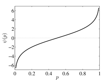
Figure 1: Graph of function $\psi(p)$ when $0\leq p\leq 1$.

The additive property of $s=\psi(p)$ is easily generalized to an arbitrary number of projections. This observation is the heart of the proposed algorithm, and in particular the initialization step. For a given direction, $j$, the projections $\pi^{j}_{k}$ are transformed into probabilities $\pi^{j}_{k}/N^{j}_{k}$ where $N^{j}_{k}=\sum_{n}W^{j}_{kn}$, and further into $s^{j}_{k}=\psi(\pi^{j}_{k}/N^{j}_{k})$. The latter is backprojected over the image to be reconstructed. The summation of these backprojections at each site $i$

$$\sigma_{i}=\sum_{j,k}{W}^{j}_{ki}s^{j}_{k}$$ (15)

or, $\bm{\sigma}={\mathbf{W}}^{\top}{\mathbf{s}}$, provides a resulting ${\bm{\sigma}}$ vector that is finally transformed back into probabilities ${\mathbf{p}}$. This transform reads

$${\mathbf{p}}=\psi^{-1}\left({\mathbf{W}}^{\top}\psi({\mathbf{D}}.{\bm{\pi}})\right)$$ (16)

where the $t$ superscript denotes transposition. Thus, up to the $\bm{\pi}$-$\mathbf{s}$ substitution, the canonical backprojection algorithm is to be used. If $\psi$ is turned into identity, the above expression reduces to a simple backprojection.

The classical FBP is based on a similar backprojection, but with the filtered signal $\bm{\pi}$ (i.e., convoluted by the inverse Fourier transform of the absolute value of the wavevector, $|k|$). This form of filter results from compensating the spreading of the back-projected values, prominent for small angles. The algebraic form of the filter is derived for a continuous distribution of angles. Let us note that the filtering could also be performed through a deconvolution on the backprojected unfiltered projection data. A similar problem of over-counting is met for a large number of projections because the same blocks of pixels appear for neighboring projection directions. The kernel to be used in the deconvolution varies with the number of projections, from the inverse Fourier of $|k|$ for a continuous distribution of angles to a Dirac distribution for two orthogonal distributions. When the maximum number of angles does not exceed 10 or 15, the filtering can simply be ignored.

As a conclusion of this section, two routes could be considered:

• The first one would consist of i) transforming the projection with the $\psi$ function, ii) applying a classical FBP algorithm from this transformed signal, iii) filtering the reconstructed image to account for the errors induced by the incomplete set of projections, iv) finally transform back the image using the $\psi^{-1}$ function, and threshold the resulting image to a value of 1/2. It is to be noted that the final step can be further simplified since thresholding the $\psi^{-1}$-transformed image at 1/2 is strictly equivalent to thresholding the untransformed image at a value of $\psi(1/2)=0$. This approach requires not too few projection angles, but is simple and fast. It works for instance in the case of a random distribution of pixels provided the fraction of 1-valued pixels matches constraints Eq. 1 as theoretically obtained by Donoho and Tanner Donoho10a ; Donoho10b . Although suited to “Type A”, this approach however does not easily allow for the incorporation of spatial correlations in the reconstructed image as required for “Type B”. It will not be further explored in the present study.

• The second option is to follow an approach similar to the iterative correction reconstruction technique, i.e., design an iterative algorithm that progressively corrects the reconstructed image. This approach is expected to be safer and more precise when the number of projections is very small, as a one step algorithm is out-of-reach. It is also a priori more demanding in terms of computation time and hence algorithmic efficiency is a critical issue. Because this approach proceeds by successive corrections, the first approach (without deconvolution) can be used to provide an initialization of the reconstructed image.

3.2 Correction

Before describing the correction step, let us briefly recall a (block-iterative) ART implementation (SART in the terminology of Ref. Kak01 , i.e., simultaneous correction of the image for each block of projection equations corresponding to a given direction, $j$, and sequential inspection of the different directions) to highlight the parallel with the proposed approach. This algorithm is based on a progressive correction of a current estimate, ${\mathbf{f}}^{(n)}$ at step $n$. The projection error ${\bm{\pi}}^{j}-{\mathbf{W}}^{j}{\mathbf{f}}^{(n)}$ along direction $j$ is computed and corrected by a uniform translation of $f$ along each ray (i.e., a backprojection) so as to cancel out this error. All projection directions are successively considered.

One interesting variant is the MART strategy MART72a ; MART72b where M stands for multiplicative. As for the SART algorithm, a block-iterative formulation, termed SMART, was introduced SMART93 ; SMART93err ; BISMART96 . This latter strategy consists of scaling (rather than translating) ${\mathbf{f}}^{(n)}$ by a constant factor along each ray to meet the projection constraint. The correction step can thus be seen as a uniform translation along each ray of $\log({\mathbf{f}}^{(n)})$ so that after correction the projection error exactly cancels out.

Section 3.1 showed that $\sigma$ is an appropriate field to apprehend the $f$ image. In the same spirit as ART and SMART, the proposed correction step is a uniform increase (or decrease) along each ray of ${\bm{\sigma}}^{(n)}$ values so that the projection constraint along that direction is exactly met. The latter increment is to be evaluated after a binarization step to produce an image ${\mathbf{f}}^{(n+1)}=H({\bm{\sigma}}^{(n+1)})$. Hence, the computation of the increment per ray is a little more demanding than in the two above SART and SMART cases, yet it can conveniently be achieved via a sorting algorithm when $\mathbf{W}$ is binary as we now discuss.

Considering a specific projection direction, $j$, and line reaching the detector at position $k$ in the above procedure, one may compute the value ${r}_{k}^{j}$ that should be subtracted to $\sigma$ so that the natural binarization of $\bm{\sigma}-\mathbf{B}^{j}{r}_{k}^{j}$ would lead to the known line-sum $\pi_{k}^{j}$, or when considering all lines indexed by $k$ in a vector notation, along the same direction $j$,

$${\mathbf{W}}^{j}H(\bm{\sigma}-\mathbf{B}^{j}{\mathbf{r}}^{j})={\bm{\pi}}^{j}$$ (17)

The solution to this non-linear equation is given by selecting the $\pi_{k}^{j}$ largest $\sigma$ values along each line $k$, as one can consider that the largest values are the ones that are the most likely to be 1-valued. Let $\sigma^{*j}_{k}$ denote the smallest of them. Alternatively, one could also consider the ${\cal N}^{j}_{k}-\pi^{j}_{k}$ smallest $\sigma$ values, and denote by $\sigma^{**j}_{k}$ the largest of them. Then any value of $r^{j}_{k}$ in the interval $\sigma^{**j}_{k}<r^{j}_{k}<\sigma^{*j}_{k}$ would fulfill condition (17). Thus it is proposed to opt for the mid-value

$$r^{j}_{k}=\frac{\sigma^{*j}_{k}+\sigma^{**j}_{k}}{2}$$ (18)

For a given projection direction, the correction of $\sigma$ along each ray is easily performed by a 1D sorting step, or more precisely by looking for the $\pi$-quantile, for which efficient algorithms exist Quantile . The resulting corrected image if binarized would fulfill the appropriate projection for the considered direction. However, presumably the projection along other directions is not correct, and thus the algorithm consists of successively considering all directions. This step is repeated twice.

Let us stress that the sorting algorithm to determine the increment $\mathbf{r}$ is specific to the case of a binary projection matrix ${\mathbf{W}}$ so that rays are decoupled from each other. In the case of a more general projection matrix, then a similar correction step could be performed but the computation of the increment $\mathbf{r}$ would be more involved, and hence less efficient. This extension has not been explored further.

The proposed algorithm shares the same property as the SMART algorithm close to 0 where $\psi(x)\sim_{x\to 0}\log(x)$. However, it also introduces a similar behavior close to $p=1$. The price to pay is that the correction is a nonlinear problem that can be solved by a sorting scheme. It is also observed that when $p$ is close to 0 or 1, a translation of $\psi$ values has a very small impact on $p$. In contrast for $\psi$ close to 0 (i.e., $p$ close to 1/2) the relative influence of a $\psi$-correction is the largest.

Even though the sought image $\mathbf{f}$ is binary, it is important to allow for intermediate values in the course of its determination. It enables to move continuously from one state to the other without having to resort to a combinatorial treatment, or being trapped within a fixed topology. The image $\mathbf{f}$, or its $\psi$-transform $\bm{\sigma}$, are natural quantities to deal with.

3.3 Regularization

Regularization is not introduced here as an extra functional to be minimized together with the projection constraints. Rather a specific iterative procedure is introduced aiming for an image $f$ lying in the constraint set, and stopping once this constraint is fulfilled. Because the solution of $\bf W\bf f=\bm{\pi}$ is generally non unique in the herein considered cases, the final image will depend on the specific procedure followed for its estimation. In some way, such a strategy can be compared to the spirit to the approach of “Binary steering” Censor . It consists of interleaving a first reconstruction step, and a second one that tends to favor either 0 or 1 for a real valued candidate for the binary image. Neither the reconstruction nor the binary steering is similar to the procedure proposed in this reference, but the spirit of alternating these two steps can be considered as qualitatively similar.

Moreover, in the early stage of the algorithm, in addition to favoring the vicinity of 0 and 1 as values for the image, high spatial frequencies will be dampened to bias $f$ toward an image containing few domains and smooth boundaries between them. Along with iterations, this high-frequency filter will progressively be tuned down, hence allowing for finer details to be introduced. However, the convergence of the algorithm relies on the fact that such a procedure is able to capture the large scale features quickly, and hence at each iteration only a small correction will be needed. In the classification of the different types of sparsity introduced in the introduction, it is observed that the last stages of the algorithm will definitely rely on the assumption that boundaries between domains will be sparse (Type B), while the first stages require that a coarse-grained image has few pixels of one “color” and thus the coarsened image should rather be of Type A. Because of this observation, we are not able to derive an operational definition of “complexity” or “simplicity” suited to the images considered hereafter, and hence we are not in a position to state precisely the conditions under which the proposed heuristic procedure converges. However, some examples shown below illustrate convergence to a satisfactory solution even if, according to the criterion of Type A complexity, no solution should have been accessible. This is due to the fact that spatial correlations reduce complexity. Provided these correlations are “gently” promoted by the procedure, a binary image may be reconstructed from few projection data. Hence, the results obtained herein and those of previous comparable studies Batenburg07 suggest that the exact reconstructability results of Type A could be extended to other types of signals when space or time correlations are considered. In this spirit, a measure of complexity derived from that proposed by Donoho and Tanner Donoho10a ; Donoho10b is tested in Section 7.

The idea of the implemented regularization is to note that the low frequency part of the image is robust with respect to the missing information, whereas the high frequency part is more fragile. In order to capture long wavelength modes, it is chosen to resort to a convolution of the current determination of the image, $f^{(n)}$, with a Gaussian kernel of characteristic size $a$, $G_{a}(\bm{x})=1/(2\pi a^{2})\exp(-\bm{x}^{2}/2a^{2})$, $g^{(n)}=G_{a}\star f^{(n)}$ where $\star$ stands for a convolution. The convoluted image can be seen as a local average over a centered domain of area $a^{2}$. Hence if the convolution image is close to 0 or 1, then it is likely that the point is inside a subregion of 0’s or 1’s respectively. In contrast, at the interface between a 0 and a 1 region, the convolution will be of order 1/2. If $g$ is substituted to $f$ as the current determination of the image, a correction step is applied that will mostly affect the boundaries of the 0 and 1 regions. However, as the procedure progresses, the reconstructed image is expected to come closer and closer to the true one, and hence, the weight to be given to the “regularization”, or a priori information, is progressively reduced. This is easily performed by reducing the extension of the Gaussian, $a$ to 1. In this limit, the convolution leaves $f^{(n)}$ essentially unchanged. Hence, the regularization initially focusses on the long wavelength components of the reconstructed image and leaves interfaces to be determined at a later stage, and progressively, regularization vanishes. In the proposed algorithm, a fixed, i.e., prescribed pace is chosen, namely $a$ is uniform and progressively reduces to 1. Thus the regularization is not defined as belonging to a specific space, not to the kernel of specific operator, but rather as a progressively less and less intrusive action on the proposed solution, first erasing the high frequency components and then preserving finer and finer scale details. The problem to be solved, namely $Wf=\pi$, $f\in\{0,1\}^{N\times N}$, is not altered, but the regularization introduced here is a way to give a hierarchy in the determined information on $f$, giving the precedence to long wavelength over short ones. This will be shown on a series of numerical (artificial) test cases, to lead efficiently to a solution. However, no other evidence than these encouraging numerical examples is offered.

Because the previous correction step involved a sorting procedure rather than a mere algebraic evolution for each pixel value, it is difficult to associate the regularization step with the correction step, and hence these two operations are performed sequentially. In the following, a matrix notation is chosen to indicate the convolution by $G_{a}(\bm{x})$, namely, $g=G_{a}\star f$ is denoted as ${\mathbf{g}}={\mathbf{G}}_{a}{\mathbf{f}}$ although in practice this convolution is performed via fast Fourier transforms. The regularization step consists of a first binarization, followed by a convolution with a Gaussian kernel, $G_{a}$

$${\mathbf{g}}={\mathbf{G}}_{a}H(\bm{\sigma})$$ (19)

Note that there is no need to transform $\bm{\sigma}$ into $\mathbf{f}$ through $\psi^{-1}$ for the binarization since $H(\bm{\sigma})=H(\mathbf{f}-0.5)$. The convolution with a Gaussian kernel is only active in the neighborhood of interface sites between 0 and 1. The smoothing of the image produced by the Gaussian convolution kernel is thus a way to ease boundary adjustments without impeding nucleation of a small cluster nor loosing the determined information on other pixels. It plays the role of a surface tension as it tends to smooth out boundaries.

The width of the Gaussian kernel, $a$, is chosen to be larger in the first steps of the algorithm, and to decrease progressively as the iteration number $n$ increases. The following choice was made in the implementation

$$a=1+\alpha^{n}(a_{0}-1)$$ (20)

with $a_{0}$ ranging typically from 2 to 4 and $\alpha$ of order 0.7-0.9. Their values are dependent on the image “complexity”. They have been chosen to allow for the quickest convergence for a series of test cases. Note that their precise value affects predominantly the convergence rate but not the quality of the result. Let us stress that in all cases the regularization part involves only very small scale modifications of the image. When $a$ approaches 1, the effect of convolution essentially vanishes. The reason for the reduction of the convolution weight is that the remaining inconsistencies between the known projection vectors $\bm{\pi}$ and the projected estimate ${\mathbf{W}}{\mathbf{f}}$ become smaller and smaller. The initial value, $a^{0}$, and its decrease rate $\alpha$ are the only adjustable parameters of the proposed procedure.

To summarize, the meta-code of the proposed procedure is given in Algorithm 1. The next section illustrates these different steps on a test case.

Input : Projection $\bm{\pi}$, Initial $a\leftarrow a_{0}$

Initialization

$\bm{\sigma}\leftarrow\bf W^{\top}\psi(\bf D\bm{\pi})$

  /* Eq. 15 */

foreach direction $j\leftarrow 1$ to $M$ do

      $\bm{\sigma}\leftarrow\bm{\sigma}+\bf B\bf r$

        /* Eq. 17 */

      

Result: $\bf f\leftarrow H(\bm{\sigma})$

Iterative correction

while $\|\bm{r}\|>\eta$ do

       $a\leftarrow 1+\alpha(a-1)$

        /* Eq. 20 */

       $\bm{\sigma}\leftarrow\psi\left({\bf G}_{a}\bf f\right)$

       for $i\leftarrow 1$ to $2$ do

            foreach direction $j\leftarrow 1$ to $M$ do

                  $\bm{\sigma}\leftarrow\bm{\sigma}+\bf B\bf r$

                    /* Eq. 17 */

                  

            

      $\bf f\leftarrow H(\bm{\sigma})$

Output : Reconstructed image $\bf f$

Algorithm 1 Algorithm consisting of two parts: Initialization, and iterative correction. $\eta$ is a small parameter controlling convergence.

4 Illustration of the procedure

All the basic ingredients of the algorithm have been defined. The resulting procedure is now illustrated on a simple example shown in Figure 2a with a rather large definition image (1 Mpixel) as compared to typical definitions from the literature. It consists of simple shape domains, with however rather sharp angles, and non convex domains. In the following the image is reconstructed from 7 projections (to be compared with the 1600 projections that would be required for a classical reconstruction). This small number of projections amounts to 0.45 % of the classical requirement.

(a) Reference

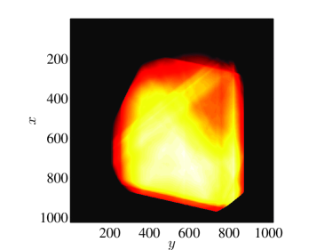
(b) $\psi$ backprojection

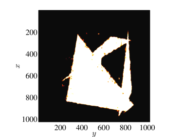
(c) 1st Correction

Figure 2: Illustration of the proposed initialization step. (a) Reference 1-Mpixel image. (b) First raw backprojection, $\psi^{-1}(\sigma)$ based on 7 projections. (c) After a single correction step. The reconstructed image are shown as a continuous gray (or color) values from black ($p=0$) to white ($p=1$). Note that the pixel error after binarization of this initialization step is only 0.82 %.

The initialization part consists of:
i) computing the $\bm{\sigma}$-image from the backprojection of $\psi$-transformed probabilities,
ii) applying a correction step.

The resulting images after each of these two steps are shown in Figures 2b and c respectively. The $\psi$ backprojection produces a $\bm{\sigma}$ image that captures the overall shape of the domains in the image, but without access to small details. It should be remembered that the $\bm{\sigma}$ map is convoluted by a discrete kernel, and no attempt is made here to perform a deconvolution. As expected all lines that do not cross the 1-valued domain have a very small $\sigma$-value. After a single correction step, the $\sigma$ values have been adjusted so that the natural binarization of the corrected image matches exactly the known projection along the last visited direction. The resulting image is shown in Figure 2c. The latter is already quite close to the original reference image. The difference between the two (fraction of pixels having the wrong $f$-value) amounts to 0.82 %.

The remainder of the procedure consists of repeating the correction step. The only difference between the successive steps is the fact that the width of the Gaussian filter progressively decreases to 1. In the present example, $a_{0}=3$, and $\alpha=0.75$.

Evaluation of the projection error $\|{\mathbf{W}}{\mathbf{f}}-\bm{\pi}\|$ is performed, and for the artificial cases considered in this study, a pixel error is also computed from the difference $\|{\mathbf{f}}_{est}-{\mathbf{f}}_{orig}\|$. If the error is less than a threshold value (or a maximum number of iterations is reached) the code terminates, otherwise a new correction step is performed starting from the obtained $\mathbf{f}$.

In the present case, only four correction steps are needed to reach an error free solution. Table 1 reports the relative pixel and projection errors as a function of iteration number.

Table 1: Convergence rate of the procedure for the example of Figure 2.

Iteration	Relative Pix. Error	Relative Proj. Error
	(%)	(%)
(init.)	0.81	1.09
1	0.23	0.42
2	0.04	0.11
3	0.001	0.004
4	0	0

(a) Iteration # 1

(b) Iteration # 2

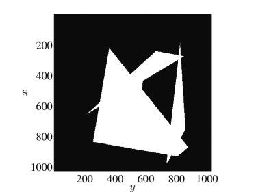
(c) Iteration # 3

Figure 3: Different stages of the reconstruction after (a) 1, (b) 2 and (c) 3 iterations. The last image differs from the original model by only 10 pixels (Figure 2(a)).

The program was written in Matlab^®, and run on a single processor PC (2.3-GHz Core i5 processor) without fancy optimization. Computation time for this 1-Mpixel image is 8.4 s.

4.1 Relation with Batenburg’s algorithm

As earlier mentioned, Batenburg proposed a rather efficient procedure for binary reconstruction Batenburg07 ; Batenburg08 . Actually the spirit of the present approach shares some similarities with that work. After initialization (performed using a standard FBP algorithm), the proposed approach by Batenburg is to find successive binary images that fulfill exactly the projection constraint along two directions, and to visit successively different pairs of projection direction. In addition to fulfilling two projection constraints, the estimate ${\mathbf{f}}^{(n)}$ is chosen to maximize its projection along a predefined direction ${\mathbf{g}}$, through the scalar product ${\mathbf{f}}^{(n)\top}{\mathbf{g}}$. Batenburg’s clever observation was to note that the satisfaction of the two projections could be rewritten as a max flow/min cut graph optimization problem. The maximization of the projection along $\mathbf{g}$ was then simply obtained as a simplex-type problem. The resulting procedure was shown to be more efficient than all available alternative algorithms. In fact the present scheme can be seen in a similar spirit with however some significant differences. First, the proposed initialization leads to a predetermination of the image much closer to the sought solution, a very helpful property for convergence. Second, the proposed correction step considers a single direction. The problem is still of simplex type, but so simple that the solution is nothing but the sorting scheme that was proposed. This results in a much simpler code. Note that Batenburg and Sijbers Batenburg09 also considered a single projection constraint at a time, later on, but this variant was found to be much less efficient than the original 2-projection constraint.

5 Multiscale acceleration

As presented so far, the algorithm has been tested in a number of different cases, always successfully, i.e., down to a zero remaining pixel error (provided enough projections are considered). However, it is possible to speed up the convergence process using a multiscale variant. The image $\mathbf{f}$ to be reconstructed can be coarse-grained by gathering 2$\times$2 pixels into super-pixels whose value is determined by a majority rule (and a random choice if the sum of pixels is equal to 2). The resulting problem is simpler in the sense that the projection information $\bm{\pi}$ is reduced by a factor of 2, but the number of pixels to be determined is reduced by a factor of 4. Hence the ratio of projection information and the unknowns is doubled. The solution to this reduced-scale problem can be re-expanded giving to each constituent pixel the same value as that of the mother super-pixel. This image can be used as the initialization of the relaxation step. Such a coarsening operation defines one level of a pyramidal construction that can be repeated up to a chosen maximum level $n_{level}$ (e.g., $n_{level}=5$ reduces the number of unknown sites by a factor of 1024). Such a multiscale strategy reduces drastically the required number of relaxation steps and thus cuts down the computation time by a significant amount (typical gains of a factor 2 or more are obtained).

Figure 4: Binarized pattern reproduced from an actual tomography. No less than 15 projections are needed to complete an error-free reconstruction using a single scale procedure. Parameter values are $a_{0}=4$, $\alpha=0.87$. (Original tomographic data were kindly provided by E. Gouillart and C. Zang Zang .)

The example shown in Figure 2 requires too few iterations for convergence to highlight the benefit of the multiscale approach. A more complicated texture binarized from an actual tomographic reconstructed image, of size $1025\times 1025$ pixels is chosen as a test case (it will be analyzed below, Figure 4). Because of the complex microstructure, a minimum number of 15 projections is needed to allow for an exact reconstruction. This should be compared with the 1500 projections needed for the original reconstruction. Without multiscale acceleration, 31 iterations are needed, resulting in a computation cost of 189 s. With 5 levels of the multiscale procedure, the same exact reconstruction is reached in 28 s i.e., about 7 times faster. The number of iterations from level 4 to 0 are successively 3, 8, 6, 3 and 3. However due to the rapid decrease of computation time with the level number, most of the computation time (more than half of it) is spent at level 0. The residual relative pixel error as a function of iteration number is shown in Figure 5. It may also be noted that using the multiscale procedure, a perfect reconstruction could be obtained for a smaller number of projections (i.e., 13).

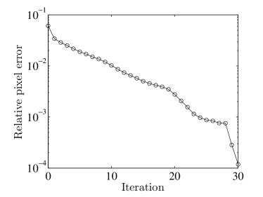
(a) Monoscale

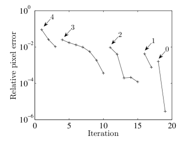
(b) Multiscale

Figure 5: Semi-log plot of the relative pixel error versus iteration number using the monoscale approach (a) reaching an error free solution at the 31-st iteration. The multiscale case is shown in (b). At the completion of a level, the error naturally increases when the coarse image is used as an initialization for the finer one. Arrows indicate the start of a given level.

6 Test Cases

Up to now, only two examples have been shown for illustration purposes. A variety of other test cases have been tried with smooth or angular shapes, equal sized domains or having a wide distribution of characteristic scales. In all the cases where the number of projections is sufficient, a successful (i.e., error-free) reconstruction was achieved, tuning parameters such as $a^{0}$ or $\alpha$ in a small range if necessary. However, depending on the complexity of the patterns, the minimum number of projections differs. When the number of projections is too small, the error saturates at a plateau value. The number of projections may be roughly related to the number of interfaces between 0 and 1 pixels, even though high curvatures also play a significant role. It has been shown mathematically that convex objects only require at most seven projections to be reconstructed exactly, and that this number can be reduced to four for specific directions Convex . Conversely, a complex pattern taken from a real tomography as shown in Figure 4 required no less than 15 (for monoscale) or 13 (for multiscale) projections for a perfect reconstruction (for a 1-Mpixel image). An a priori evaluation of the “complexity” of an image, and the minimum number of projections needed to reconstruct it, is an interesting and important question that deserves further studies.

In order to illustrate the performances of the proposed algorithm, we reproduced a series of tests initially proposed by Batenburg Batenburg07 . In the latter reference, a detailed comparison of the algorithm proposed by the author with two of the most powerful approaches proposed so far. More precisely, the first one is the extension proposed by Weber et al. Weber03 , of the linear programming algorithm of Fishburn et al. Fishburn97 , and the second one is a greedy algorithm without any smoothness prior Gritzmann00 .

All those benchmark tests are carried out on $257\leavevmode\nobreak\ \times\leavevmode\nobreak\ 257$-“pixel” lattices, and for each type of pattern, the numbers indicated in the tables correspond to an average over 200 random samples. Although we tried to remain as close as possible from the initially proposed references, some adjustments were necessary. All the objects present in the binary image are to fit in a circle inscribed in the square. In doing so, the number of objects is preserved rather than their density (so that if the number of 0-1 interfaces is a crucial parameter, complexity is not altered). For a dilute collection of objects such interface sites remain the same. A second difference worth mentioning is the fact that the projections used in the present analysis have a fixed size equal to the width of a pixel in the binary image. In contrast, in Ref. Batenburg07 , all distinct point-wise projections were distinguished, so that the actual amount of information (i.e., number of line-sums) may be significantly larger than the one used in the present case (when the angle tangent does not coincide with a fraction of low integers).

6.1 Polygon test cases

The first test case was constructed from the union of $n$ convex polygons. Each polygon is constructed from a random set of $p$ points within the largest inscribed circle, from which a convex hull is considered. The two parameters $(n,p)$ thus characterize the image. Three such cases where considered, ranging from a single $n=1$ convex polygon (with a large number of points $p=25$ although fewer actually are vertices of the convex envelope), to a large number $n=25$ of such polygons constructed from few points ($p=4$). The intermediate case consists of $n=5$ polygons built from $p=8$ points. The first case is an elementary problem, the two subsequent examples exhibit details and non convexity that are much more difficult to capture. Figure 6 shows an example of the three choices of $(n,p)$ values.

Those examples were then analyzed with a variable number of projections $M$. For each of them, the proportion of perfect reconstructions (out of the 200 trials) was recorded together with the projection error (i.e., the sum of absolute value of differences between original data and reconstructed projections, averaged over all 200 samples), and the pixel error (i.e., the number of pixel differing in the binary image and its reconstruction, averaged over all 200 samples). Finally the computation time is recorded. Note that the same set of parameters was chosen to complete the analysis, namely, three coarse-graining steps were considered, and the total number of iterations per scale was limited to a maximum value of 20 (or less if perfect reconstruction is reached earlier). Data extracted from Ref. Batenburg07 are reported in Table 2, whereas the corresponding result for the present algorithm is given in Table 3.

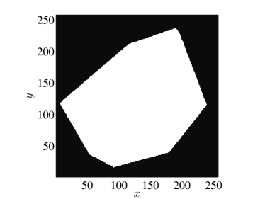
(a) $n=1$, $p=25$

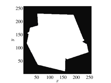
(b) $n=5$, $p=8$

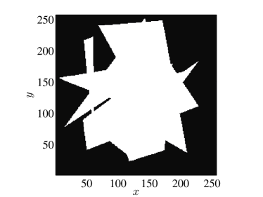
(c) $n=12$, $p=4$

Figure 6: Polygon test cases for the three sets of parameters $(n,p)$ used.

Table 2: Polygon test cases reproduced from Ref. Batenburg07 .

$n$	$p$	$M$	# perfect (%)		Proj. error		Pix. error		Time (s)
1	25	3	93.	5	0.	5	24.	0	13
		4	100.	0	0.	0	0.	0	11
5	8	3	29.	5	32.	0	538.	0	14
		4	100.	0	0.	0	0.	0	11
		5	100.	0	0.	0	0.	0	10
12	4	4	95.	0	12.	0	62.	0	18
		5	100.	0	0.	0	0.	0	18
		6	100.	0	0.	0	0.	0	14

Table 3: Polygon test cases with the present method (number of levels $=3$, $a_{0}=4$, $\alpha=0.87$).

$n$	$p$	$M$	# perfect (%)		Proj. error		Pix. error		Time (s)
1	25	3	92.	5	1.	0	3.	0	0.36
		4	99.	0	0.	0	0.	6	0.45
5	8	3	63.	5	1.	0	1.	7	0.50
		4	99.	0	1.	0	5.	7	0.43
		5	100.	0	0.	0	0.	0	0.43
12	4	4	90.	0	2.	0	21.	0	1.92
		5	97.	5	1.	0	1.	3	1.31
		6	100.	0	0.	0	0.	0	1.04

Although the geometry of this test case is simple, the very small number of projection directions makes the problem difficult. In particular, even without projection error, the image may not be reconstructed perfectly, (see e.g., $n=1$, $p=25$, $M=4$ in Table 3). The proportion of perfect reconstructions is comparable in Ref. Batenburg07 and with the proposed algorithm, apart for the $n=5$, $p=8$ and $M=3$ case, where the present code has about half unperfect reconstructions. In most other cases the differences are not significant, as the errors are not weighted in this criterion. When considering the mean projection error, it is observed that it never exceeds 2 with the present approach. The mean pixel error is 21 wrong pixels in the worst case. It is to be stressed that this represents only an extremely small fraction, $3\times 10^{-4}$, of pixels. Thus in terms of errors, the proposed approach performs generally better than Ref. Batenburg07 . Finally, in terms of computation time, we observe a reduction in the computation time by a factor of order 10 to 20. Let us stress that this latter comparison is fragile, as it amounts to compare codes written in different languages, and run on different computers. In the present case however, the code was not optimized, and was run on a standard laptop computer.

6.2 Ellipse test case

The second series of tests consists of the union of $n$ random ellipses whose principal axes are picked at random in the interval $[r_{min},r_{max}]$. The principal axis of the ellipse is also chosen randomly with a uniform distribution over $[0,\pi]$ (i.e., isotropic distribution). Hence a test case is characterized by three parameters $(n,r_{min},r_{max})$. Figure 7 shows an example of the five cases considered in the following series. Here again, the number $M$ of projection directions was varied depending on the complexity of the case. The image size was here again $257\leavevmode\nobreak\ \times\leavevmode\nobreak\ 257$ “pixels.”

As in the previous case, 200 samples were generated for each set of parameters, and averages over these samples are reported in Tables 4 (reproduced from Ref. Batenburg07 ) and 5 for the proposed algorithm. Let us note that we reproduce here only global numbers and did not consider statistics over “successful” reconstructions.

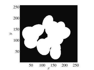
(a) $n=15$, $r_{min}=20$, $r_{max}=40$

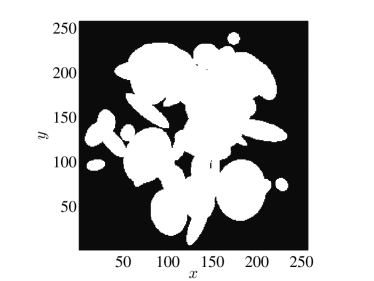
(b) $n=50$, $r_{min}=5$, $r_{max}=35$

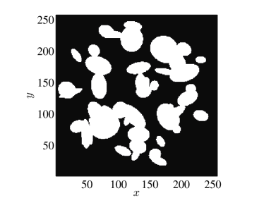
(c) $n=50$, $r_{min}=5$, $r_{max}=25$

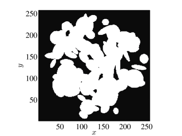
(d) $n=100$, $r_{min}=5$, $r_{max}=25$

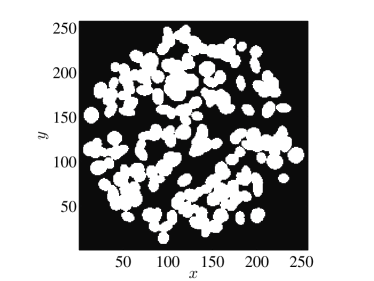
(e) $n=200$, $r_{min}=5$, $r_{max}=10$

Figure 7: An example for the ellipse test cases for the five sets of parameters $(n,r_{min},r_{max})$.

Table 4: Ellipse test case reproduced from Ref. Batenburg07 .

$n$	$r_{min}$	$r_{max}$	$M$	# perfect (%)		Proj. error		Pixel error		Time(s)
15	20	40	4	38.	5	170.	0	3257.	0	36
			5	100.	0	0.	0	0.	0	19
			6	100.	0	0.	0	0.	0	13
50	5	35	5	4.	5	737.	0	7597.	0	57
			6	56.	5	577.	0	2779.	0	43
			7	61.	0	5.	9	1.	2	22
			8	79.	5	7.	5	1.	3	20
50	5	25	6	17.	5	1202.	0	6510.	0	54
			7	54.	5	521.	0	1289.	0	37
			8	81.	0	6.	3	1.	1	21
			9	65.	0	13.	2	1.	9	21
100	5	25	7	5.	5	1589.	0	4455.	0	61
			8	31.	5	270.	0	457.	0	40
			9	36.	5	31.	0	4.	5	31
200	5	10	12	2.	5	6699.	0	6157.	0	117
			14	13.	5	107.	0	9.	0	68
			16	13.	0	131.	0	9.	5	48

Table 5: Ellipse test cases with the proposed algorithm (number of levels $=3$, $a_{0}=4$, $\alpha=0.87$).

$n$	$r_{min}$	$r_{max}$	$M$	# perfect (%)		Proj. error		Pixel error		Time(s)
15	20	40	4	83.	5	2.		41.	2	2.0
			5	99.	5	0.		0.	005	1.4
			6	100.	0	0.		0.		1.3
50	5	35	5	73.	0	19.		497.		6.3
			6	97.	5	2.		15.		5.1
			7	100.	0	0.		0.		4.4
			8	99.	5	0.		0.	4	4.4
50	5	25	6	46.	5	43.		1665.		8.6
			7	97.	0	2.		45.		5.6
			8	99.	5	1.		15.		5.3
			9	100.	0	0.		0.		4.6
100	5	25	7	90.	5	5.		79.		8.3
			8	99.	0	1.		10.		7.9
			9	99.	5	0.		0.	02	8.1
200	5	10	12	22.	5	152.		2472.		19.8
			14	98.	5	3.		5.		14.1
			16	98.	5	3.		5.		14.8

The ellipse test cases are more demanding than the polygon ones, and require a larger number of projections. The chosen number of projections is clearly for the smaller values at the lower limit of the minimum value for a decent reconstruction success rate. Only the first series with fifteen ellipses and four projections can be tackled safely with 100-% success for 5 and 6 projections in Table 4 from Ref. Batenburg07 . The last series (200 ellipses) can hardly be considered as satisfactory with at best 13-% success rate. In contrast, we observe that, with the present approach, all series reach a success rate above 98.5-% provided enough projections are taken into account. The projection and pixel errors are systematically much smaller with the present approach, even when the overall success rate is low. Finally the computation time is reduced by a factor from 5 to 10 from that reported by Batenburg Batenburg07 .

For all the test cases, the proposed algorithm is shown to perform better than Batenburg’s procedure both in terms of lower residual error (projection and reconstructed image) and lower computation time.

7 Complexity

Considering the previous results, let us try to formulate a measurement of “complexity” relevant for our algorithm. As mentioned in the introduction, Donoho and Tanner Donoho10a ; Donoho10b have derived an appropriate measurement of complexity in the case where no spatial correlation are present in the image to be reconstructed. In this case, complexity has to be a function of the fraction of 1-pixels, $p$, (or 0-pixels whichever is the minority value). Moreover, a critical value $p_{c}$ given in Eq. 1 allows one to distinguish solvable problems where $p<p_{c}$ from those where information is lacking, $p>p_{c}$. Thus $\chi_{A}=p/p_{c}=2p\delta\log(\delta)$ can be seen as a measure of complexity for Type A problems where $\delta=N/M$ is the undersampling ratio.

No such result has been derived for Type B problems, where boundaries play somehow the role played by minority pixels in Type A. If the fraction of boundary “bonds” (i.e., pairs of neighbouring pixels having a different value) $p_{b}$ is introduced, it is natural to consider

$$\chi_{B}=p_{b}\delta\log(\delta)$$ (21)

as a candidate for quantifying the image complexity for Type B. Figure 8 is an attempt to quantify the final pixel error as a function of the average $\chi_{B}$ measured from each image series. On this graph, all the test cases reported earlier (polygons and ellipses) have been collected, as well as the AlCu tomographic image. This plot seems to indicate that small values of $\chi_{B}\leq 3.5$ can be solved exactly, while values above 4 may be out of reach of the present algorithm. Note however that there is no formal justification for this choice concerning the measure of complexity.

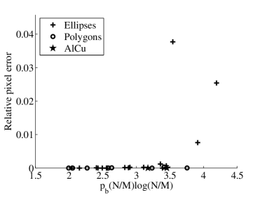
Figure 8: Relative pixel error as a function of the proposed measure of complexity, $\chi_{B}$.

8 Robustness with respect to noise

To test the robustness of the proposed methodology with respect to noise, only the case of the microstructure shown in Figure 4 has been chosen as representative of a challenging case, in particular considering its size (i.e., 1024$\times$1024 pixels), and its complex geometry. The physics of noise generation in the projections reflects a number of different phenomena. The ambition is not to reproduce a specific noise, but rather to test the robustness of the algorithm. Thus it is chosen to add a Gaussian white noise to the projection data. The noise is characterized by its Signal to Noise Ratio, SNR, such that

$$\mathrm{SNR}=20\log_{10}\left(\frac{\langle\pi\rangle}{\eta}\right)$$ (22)

where $\eta$ is the standard deviation of the noise.

The number of projections is $M=15$, and a standard set of parameters was chosen to deal for all SNRs. The number of scales was chosen to be 4, with 30 iterations per scale. The regularization length scale was chosen to be larger than in the preceding examples $a_{0}=10$, and hence with a faster decay rate $\alpha=0.8$. At the end of the prescribed number of iterations, the relative pixel and projection errors are computed. Relative means here that the pixel error is normalized by the total number of pixels in the reconstructed disk, and the projection error is normalized by the mean projection data, $\langle\pi\rangle$.

Figure 9 shows the change of both errors as functions of the SNR. It is observed that both errors have a similar evolution, and although the process is intrinsically susceptible to noise (because of the low level of information provided), convergence to decent reconstruction is still achieved. For a 1% level of fluctuations in the projection data (SNR$=40$), the relative pixel error is about 3%. Let us emphasize the fact that spatial regularization is essentially active in the first few iterations (when $a$ is significantly larger than 1) and hence no filter is applied in the last stages apart from the projection constraints that are corrupted by noise. A post-processing of the data to remove isolated pixels for instance (or involving a more elaborate filtering) is able to reduce significantly the resulting error. This section is included to document the robustness of the proposed procedure, but the latter has not been designed to be especially immune to noise, but rather to allow for an efficient reconstruction for a low number of projections $M$.

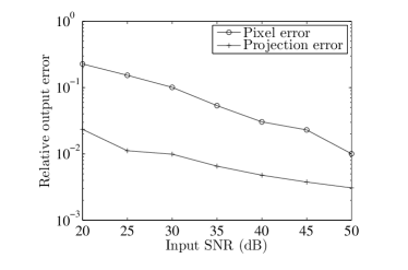
Figure 9: Evolution of pixel or projection errors at the end of the reconstruction as a function of the noise signal ratio, SNR.

9 Conclusion

A novel binary reconstruction algorithm has been introduced. It is based on a nonlinear transformation of the probability for a site to be 1-valued. The proposed initialization step is a mere backprojection applied to a non-linear transformed projection data, followed by a correction step. A correction scheme to meet the projection constraints and involving a minimal regularization procedure (binarization and convolution by a small width Gaussian kernel) allows error-free binary reconstructions to be achieved for a variety of examples of large image sizes (examples of 1-Mpixel images have been shown). A multiscale version speeds up convergence. A detailed comparison with a series of test cases provided in Ref. Batenburg07 shows that the proposed algorithm achieves very good performances (superior success rate and lower computation time).

Let us emphasize that the number of required projection data can be as low as 1 % of the required number for standard reconstructions. This has direct consequences in terms of X-ray dose reduction for medical applications (provided the severe constraint (or approximation) or looking for a binary image can be acceptable), or for fast-imaging where acquisition time is limited.

An appealing route is to provide an efficient computer implementation of the proposed algorithm. Up to now a basic Matlab^® code has been used on a simple processor PC. GPU implementation is expected to offer much higher performances.

Finally, extensions of such approaches to discrete (rather than binary) images is also very challenging as it would open new perspectives for applications, going beyond the very restrictive frame of binary images. In a similar spirit, the application of the proposed binary algorithm to images that are not binary is an interesting question to be addressed.

- (1) Atkinson C., Soria J., An efficient simultaneous reconstruction technique for tomographic particle image velocimetry, Exp. Fluids 47, 553–568, (2009)
- (2) J. Baruchel, J.-Y. Buffière, P. Cloetens, M. di Michiel, E. Ferrié, W. Ludwig, E. Maire, L. Salvo, Advances in synchrotron radiation microtomography, Scripta Mat., 55, 41–46, (2006)
- (3) K.J. Batenburg, A network flow algorithm for reconstructing binary images from discrete X-rays, J. Math. Imaging Vis. 27, 175–191, (2007)
- (4) K.J. Batenburg, A network flow algorithm for reconstructing binary images from continuous X-rays, J. Math. Imaging Vis. 30, 231–248, (2008)
- (5) K.J. Batenburg, J. Sijbers, Generic iterative subset algorithms for discrete tomography, Discrete Applied Mathematics, 157, 438–451, (2009)
- (6) S. Basu, Y. Bresler, Filtered backprojection reconstruction algorithm for tomography, IEEE Trans. Image Proc., 9, 1760–1773, (2000)
- (7) S. Basu, Y. Bresler, Error analysis and performance optimization of fast hierarchical backprojection algorithms, IEEE Trans. Image Proc., 10, 1103–1117, (2001)
- (8) C.L. Byrne, Iterative image reconstruction algorithms based on cross-entropy minimization, IEEE Trans. Image Processing, 2, 96–103, (1993)
- (9) C.L. Byrne, Erratum and addendum to ’Iterative image reconstruction algorithms based on cross-entropy minimization’, IEEE Trans. Image Processing, 4, 226–227, (1995)
- (10) C.L. Byrne, Iterative algorithms for deblurring and deconvolution with constraints, Inverse Problems, 14, 1455–1467 (1998)
- (11) C.L. Byrne, Block-iterative methods for image reconstruction from projections, IEEE Trans. Image Processing, 5, 792–794, (1996)
- (12) E.J. Candès, J. Romberg, T. Tao, Robust uncertainty principles: exact signal reconstruction from highly incomplete frequency information, IEEE Trans. Inform. Theory, 52, 489–509, (2006)
- (13) B.M. Carvalho, G.T. Herman, S. Matej, C. Salzberg, E. Vardi, Binary tomography for triplane cardiography, in IPMI’99, A. Kuba et al. (Eds.), LNCS 1613, 29–41, (Springer-Verlag, Berlin), (1999)
- (14) Y. Censor, Binary steering in discrete tomography reconstruction with sequential and simultaneous iterative algorithms, Linear Algebra and its Applications, 339, 111–124, (2001)
- (15) J.N. Darroch, D. Ratcliff, “Generalized iterative scaling for log linear models”, Annals Math. Statist., 43, 1470–1480, (1972)
- (16) D.L. Donoho, “Neighborly polytopes and sparse solution of underdetermined linear equations”, Technical Report, Department of Statistics, Stanford University, (2004)
- (17) D.L. Donoho, J. Tanner, “Counting the faces of randomly-projected hypercubes and orthants with applications”, Discrete Comput. Geom., 43, 522–541, (2010)
- (18) D.L. Donoho, J. Tanner, “Precise Undersampling Theorems”, Proceedings of the IEEE, 98, 913–924, (2010)
- (19) G.E. Elsinga, F. Scarano, B. Wieneke, B.W. van Oudheusden, Tomographic particle image velocimetry, Exp Fluids 41, 933–947, (2006)
- (20) P. Fishburn, P. Schwander, L. Shepp, R. Vanderbei, The discrete Radon transform and its approximate inversion via linear programming, Discrete Appl. Math., 75, 39–61, (1997)
- (21) R.J. Gardner, P. Gritzmann, Discrete tomography: determination of finite sets by X-rays, Trans. Amer. Math. Soc., 349, 2271–95, (1997)
- (22) R.J. Gardner, P. Gritzmann, D. Prangenberg, On the computational complexity of reconstructing lattice sets from their X-rays, Discrete Math., 202, 45–71, (1999)
- (23) R.J. Gardner, Geometric tomography, Cambridge University Press, New York (2006)
- (24) E. Gouillart, F. Krzakala, M. Mezard, L. Zdeborová, Belief Propagation Reconstruction for Discrete Tomography, Inverse Problems, 29, 035003, (2013)
- (25) P. Gritzmann, S. de Vries, M. Wiegelmann, Approximating binary images from discrete X-rays, SIAM J. Optim., 11, 522–546, (2000)
- (26) G.T. Herman, A. Lent, Iterative reconstruction algorithms, Comput. Biol. Med. 6, 273–294, (1976)
- (27) G.T. Herman and A. Kuba (eds.), Discrete tomography: foundations, algorithms and applications, Bikhäuser, Boston (1999)
- (28) G.T. Herman and A. Kuba (eds.), Advances in discrete tomography and its applications, Bikhäuser, Basel (2007)
- (29) A.C. Kak and M. Slaney, Principles of computerized tomographic imaging, SIAM, (2001)
- (30) H.Y. Liao, G.T. Herman, Direct image reconstruction-segmentation as motivated by electron microscopy, G.T. Herman and A. Kuba (eds.), Advances in discrete tomography and its applications, Bikhäuser, Basel (2007)
- (31) G.S. Manku, S. Rajagopalan, B.G. Lindsay, Approximate medians and other quantiles in one pass and with limited memory, ACM SIGMOD, 12, 426-435, (1998)
- (32) R.M. Mersereau, Direct Fourier transform techniques in 3-D image reconstruction, Comput. Biol. Med., 6, 247–258, (1976)
- (33) D. Needell, R. Ward, Stable image reconstruction using total variation minimization, SIAM Journal on Imaging Sciences, 6, 1035–1058 (2013).
- (34) P. Schmidlin, Iterative separation of sections in tomographic scintigrams, Nucl. Med., 15, (1), (1972), Schatten Verlag, Stuttgart.
- (35) S. Sina Jafarpour, W. Xu, B. Hassibi, A.R. Calderbank, “Efficient and robust compressed sensing using optimized expander graphs”, IEEE Trans. Inform. Theory, 55, 4299–4308, (2009)
- (36) C.H. Slump, J.J. Gerbrands, A network flow approach to reconstruction of the left ventricle from two projections, Comput. Gr. Im. Proc., 18, 18–36, (1982)
- (37) L. Varga, P. Balázs, A. Nagy, Direction-dependency of a binary tomographic reconstruction algorithm, R.P. Barneva et al. (Eds.): CompIMAGE 2010, Lect. Notes in Comput. Sci. 6026, 242–253, (2010)
- (38) S. Weber, C. Schnörr, J. Hornegger, A linear programming relaxation for binary tomography with smoothness priors, Electron. Notes Discrete Math., 12, (2003).
- (39) S. Weber, A. Nagy, T. Schüle, C. Schnörr, A. Kuba, A benchmark evaluation of large-scale optimization approaches to binary tomography, A. Kuba, L.G. Nyúl, and K. Palágyi (Eds.) Lect. Notes in Comput. Sci. 4245, 146–156, (2006)
- (40) A. Yang, A. Ganesh, S. Sastry, Y. Ma, Fast -minimization algorithms and an application in robust face recognition: a review, 17th IEEE Int. Conf. Image Proc. (ICIP), 1849–1852, (2010)
- (41) Zang C., Private communication, 2011.