Evolutionary consequences of assortativeness in haploid genotypes

Abstract

We study the evolution of allele frequencies in a large population where random mating is violated in a particular way that is related to recent works on speciation. Specifically, we consider non-random encounters in haploid organisms described by biallelic genes at two loci and assume that individuals whose alleles differ at both loci are incompatible. We show that evolution under these conditions leads to the disappearance of one of the alleles and substantially reduces the diversity of the population. The allele that disappears, and the other allele frequencies at equilibrium, depend only on their initial values, and so does the time to equilibration. However, certain combinations of allele frequencies remain constant during the process, revealing the emergence of strong correlation between the two loci promoted by the epistatic mechanism of incompatibility. We determine the geometrical structure of the haplotype frequency space and solve the dynamical equations, obtaining a simple rule to determine equilibrium solution from the initial conditions. We show that our results are equivalent to selection against double heterozigotes for a population of diploid individuals and discuss the relevance of our findings to speciation.

I Introduction

While the origin of species has always been a central subject in evolutionary biology, the large number of recent empirical and theoretical developments has renewed the interest in the area (Coyne and Orr, 2004; gavrilets_2004, ; Butlin et al., 2012; Nosil, 2012). Individual-based simulations, in particular, have been successful in fostering relevant discussions in speciation (higgs1991, ; higgs1992, ; kondra1998, ; Dieckmann and Doebeli, 1999; Gavrilets, 1999; doursat2008, ; Doorn et al., 2009; fitzpatrick2009, ; de_aguiar_global_2009, ; ashlock2010, ; kopp2010, ; melian2011, ; desjardins2012, ). Specifically, simulations in which mating is restricted by spatial and genetic distances have been able to describe empirical patterns of species diversity (de_aguiar_global_2009, ) and within-species genetical diversity (Martins et al., 2013).

One of the simplest ways of introducing assortativeness in mating in a individual-based simulation is to attribute haploid genomes with $B$ biallelic loci to individuals and allow them to mate only if the genomes differ in no more than $G$ loci (Gavrilets et al., 2000; de_aguiar_global_2009, ; Martins et al., 2013). This approach considers that mate choice often relies on multiple cues that are determined genetically (Candolin, 2003). In the case of assortative mating, we assume that individuals have a certain tolerance to differences when choosing a mate, however if the other individual is too different, it will no longer be considered a potential mate. Under these assumptions, reproductive isolation was shown to be maintained among demes in the presence of sufficiently low migration rates (Gavrilets et al., 2000). Spatially explicit versions of this process have also been studied doursat2008 ; fitzpatrick2009 ; de_aguiar_global_2009 ; ashlock2010 ; melian2011 ; Martins et al. (2013) and, in particular, speciation was shown to emerge spontaneously if mating is also constrained by the spatial distance (doursat2008, ; de_aguiar_global_2009, ; ashlock2010, ; Martins et al., 2013).

In order to reflect the dynamics of evolving populations, most simulations need to incorporate several ingredients simultaneously, such as mutation, genetic drift, recombination, assortativeness in mating and individual’s movement and spatial positioning. Gavrilets Gavrilets (1999) proposed and analysed a number of simplified mathematical models that are closely related to these simulations, including selection, mutation, drift and population structure. These more realistic approaches to speciation do not allow for the detailed understanding of how each of the mechanisms involved contribute to the emergence and maintenance of reproductive isolation.

To construct a dynamical theory that accounts for the predictions of the model described in de_aguiar_global_2009 and other similar models, it is important to understand the roles of their different ingredients and to validate their generality. It has already been shown that separation of individuals into males and females does not introduce important effects in the conditions for speciation baptestini_2013 ; schneider_2012 , originally based on hermaphrodite populations. In this paper we focus on the effect of genetic incompatibility and work out the theory for infinitely large populations with two biallelic loci ($B=2$) without mutations. Genetic incompatibilities will be implemented by allowing reproduction only if the alleles from the parents differ at most in one locus ($G=1$). This is the simplest system for which the genetical mechanism of interest may be implemented. We will show that this process leads to evolution by changing the allele frequencies and that it is one of the main ingredients in the process of speciation studied in (de_aguiar_global_2009, ). Despite the changes in all allele frequencies, we will demonstrate that a certain combination of frequencies from the two loci remain constant during the evolution, revealing a strong correlation between the loci introduced by the genetic mating restriction.

The paper is organized as follows. In section II we describe the reproductive mechanism employed in the dynamics. In section III we characterize the evolution of a population subjected to no mating restrictions (random mating), which is similar to the Hardy-Weinberg (HW) equilibrium. The mathematical implications of the genetic restriction, including the description of equilibria and their features, are analyzed in section IV. Finally, in section V we expose our conclusions and discuss the possible evolutionary impacts of our results. Mathematical technicalities not strictly essential to the discussion are included in the appendices.

II Reproductive mechanism

Consider a population of $N$ hermaphrodite individuals with haplotypes $AB$, $Ab$, $aB$, and $ab$ ($A$ and $a$ being the alleles at the locus 1, and $B$ and $b$ the alleles at the locus 2), whose composition at the generation $t$ is characterized by the numbers $N_{AB}$, $N_{Ab}$, $N_{aB}$ and $N_{ab}$ ($\sum_{u^{\prime},u^{\prime\prime}}N_{u^{\prime}u^{\prime\prime}}=N$, with $u^{\prime}=\{A,a\}$ and $u^{\prime\prime}=\{B,b\}$). All possibles encounters between members of this generation give an offspring which will be a member of the generation $t+1$ with a probability $r_{h_{1}\!:h_{2}}$, $h_{1}$ and $h_{2}$ being the paternal haplotypes (we include in $r_{h_{1}\!:h_{2}}$ both effects of compatibility of the parents and the viability of the new born individual). By assuming no overlap among generations, the contributions to the individuals with haplotype $AB$ at generation $t+1$ can be inferred from Table 1.

$$\begin{array}[]{c|c|c}\text{Paternal haplotypes}&\text{Number of encounters}&\text{Fraction of successful}\\ &&\text{$AB$ offspring}\\ \hline\cr AB\times AB&\frac{1}{2}N_{AB}\times(N_{AB}-1)&r_{AB:AB}\\ AB\times Ab&N_{AB}\times N_{Ab}&1/2\times r_{AB:Ab}\\ AB\times aB&N_{AB}\times N_{aB}&1/2\times r_{AB:aB}\\ AB\times ab&N_{AB}\times N_{ab}&1/4\times r_{AB:ab}\\ Ab\times aB&N_{Ab}\times N_{aB}&1/4\times r_{Ab:aB}\\ \end{array}$$

Table 1: Production of individuals with haplotypes $AB$ at generation $t+1$, through encounters between individuals of the generation $t$.

The number of $AB$ individuals at time $t+1$ obeys thus the equation

$$N_{AB}^{t+1}=\frac{N_{AB}(N_{AB}-1)}{2}r_{AB:AB}+\frac{N_{AB}N_{Ab}}{2}r_{AB:Ab}+\frac{N_{AB}N_{aB}}{2}r_{AB:aB}+\frac{N_{AB}N_{ab}}{4}r_{AB:ab}+\frac{N_{Ab}N_{aB}}{4}r_{Ab:aB}$$ (1)

Equivalent tables allow to obtain evolution equations for the remaining haplotypes

$$N_{Ab}^{t+1}=\frac{N_{Ab}(N_{Ab}-1)}{2}r_{Ab:Ab}+\frac{N_{AB}N_{Ab}}{2}r_{AB:Ab}+\frac{N_{Ab}N_{ab}}{2}r_{Ab:ab}+\frac{N_{AB}N_{ab}}{4}r_{AB:ab}+\frac{N_{Ab}N_{aB}}{4}r_{Ab:aB}$$ (2)

$$N_{aB}^{t+1}=\frac{N_{aB}(N_{aB}-1)}{2}r_{aB:aB}+\frac{N_{AB}N_{aB}}{2}r_{AB:aB}+\frac{N_{aB}N_{ab}}{2}r_{aB:ab}+\frac{N_{AB}N_{ab}}{4}r_{AB:ab}+\frac{N_{Ab}N_{aB}}{4}r_{Ab:aB}$$ (3)

$$N_{ab}^{t+1}=\frac{N_{ab}(N_{ab}-1)}{2}r_{ab:ab}+\frac{N_{Ab}N_{ab}}{2}r_{Ab:ab}+\frac{N_{aB}N_{ab}}{2}r_{aB:ab}+\frac{N_{AB}N_{ab}}{4}r_{AB:ab}+\frac{N_{Ab}N_{aB}}{4}r_{Ab:aB}$$ (4)

In the following sections we analyze the dynamics of the haplotype frequencies $p_{u^{\prime}u^{\prime\prime}}\equiv N_{u^{\prime}u^{\prime\prime}}/N$ in the infinite limit of the population size. For each different scenario we specify the values of the probabilities $r_{h_{1}\!:h_{2}}$ by setting the total number of individuals constant along generations.

III The non restricted case

This section summarizes the outcomes for the case of no genetic restrictions. Although some of the results described in here can be found in the literature (see for example crow_introduction_1970 ; ewens ), the following discussion is fundamental as a reference for comparing the results presented next.

If random mating is assumed, $r_{h_{1}\!:h_{2}}=r$ for every encounter. Substituting in equations (1-4) and summing up, one obtains

$$N^{t+1}=rN(N-1)/2\equiv N,$$ (5)

so that $r=2/N$ for very large populations. By introducing $D=p_{AB}p_{ab}-p_{Ab}p_{aB}$, the so called linkage disequilibrium, and after some algebra, equations for the haplotype frequencies read

$$p_{AB}^{t+1} =p_{AB}-\frac{1}{2}D$$ (6)

$$p_{Ab}^{t+1} =p_{Ab}+\frac{1}{2}D$$ (7)

$$p_{aB}^{t+1} =p_{aB}+\frac{1}{2}D$$ (8)

$$p_{ab}^{t+1} =p_{ab}-\frac{1}{2}D$$ (9)

,

from which one immediately sees that a sufficient condition for the equilibrium is $D=0$, or $p_{AB}p_{ab}=p_{Ab}p_{aB}$. Notice that the quantities

$$\tilde{p}_{A}= p_{AB}+p_{Ab}$$ (10)

$$\tilde{p}_{a}= p_{aB}+p_{ab}$$ (11)

$$\tilde{p}_{B}= p_{AB}+p_{aB}$$ (12)

$$\tilde{p}_{b}= p_{Ab}+p_{ab},$$ (13)

representing the frequencies of the four available alleles, remain constant from the first generation. This is also the case in the HW equilibrium context, however it should be emphasized that in the present framework there are two independent allele frequencies (because $\tilde{p}_{A}+\tilde{p}_{a}=\tilde{p}_{B}+\tilde{p}_{b}=1$) in contrast to the HW equilibrium where the only independent variable is the frequency of one of the two available alleles.

The time dependence of the haplotype frequencies can be obtained analytically (see appendix A). Here we just look for a relationship between the haplotype and the allele frequencies.We start calculating $D$ at time $t+1$,

$$D^{t+1}=(p_{AB}-\frac{1}{2}D)(p_{ab}-\frac{1}{2}D)-(p_{Ab}+\frac{1}{2}D)(p_{aB}+\frac{1}{2}D)=\frac{1}{2}D,$$ (14)

whose solution is simply

$$D=\frac{1}{2^{t}}D^{0},$$ (15)

$D^{0}$ being the initial value of $D$. Combining (10-12) and (6-9), it is possible to deduce the following relationships (see appendix B)

$$p_{AB} =\tilde{p}_{A}\tilde{p}_{B}+D=\tilde{p}_{A}\tilde{p}_{B}+\frac{1}{2^{t}}D^{0}$$ (16)

$$p_{Ab} =\tilde{p}_{A}\tilde{p}_{b}-D=\tilde{p}_{A}\tilde{p}_{b}-\frac{1}{2^{t}}D^{0}$$ (17)

$$p_{aB} =\tilde{p}_{a}\tilde{p}_{B}-D=\tilde{p}_{a}\tilde{p}_{B}-\frac{1}{2^{t}}D^{0}$$ (18)

$$p_{ab} =\tilde{p}_{a}\tilde{p}_{b}+D=\tilde{p}_{a}\tilde{p}_{b}+\frac{1}{2^{t}}D^{0}$$ (19)

Accordingly, the haplotype frequencies reach an equilibrium asymptotically and, as in the case of the HW equilibrium, is related to the constant alleles frequencies,

$$p_{AB}^{\rm eq} =\tilde{p}_{A}\tilde{p}_{B}$$ (20)

$$p_{Ab}^{\rm eq} =\tilde{p}_{A}\tilde{p}_{b}$$ (21)

$$p_{aB}^{\rm eq} =\tilde{p}_{a}\tilde{p}_{B}$$ (22)

$$p_{ab}^{\rm eq} =\tilde{p}_{a}\tilde{p}_{b}$$ (23)

It is important to remark the asymptotic behavior of the haplotype frequencies toward the equilibrium (equations (16-19)), in contrast to HW theorem in which the equilibrium of the genotype frequencies is attained in one generation.

IV Genetically restricted mating

To mathematically describe the mating restriction imposed to individuals differing in more than one allele, we simply redefine the compatibility-viability rate as follows

$$r_{h_{1}:h_{2}}=\left\{\begin{array}[]{cc}0&h_{1}\!:\!h_{2}=AB\!:\!ab\;\text{ or }\;h_{1}\!:\!h_{2}=Ab\!:\!aB\\ r^{\prime}&{\rm otherwise}\end{array}\right.$$ (24)

Following the procedure of section III, we obtain

$$r^{\prime}=\frac{2}{N}\frac{1}{1-2\Delta}$$ (25)

with

$$\Delta\equiv\frac{N_{AB}N_{ab}+N_{Ab}N_{aB}}{N^{2}}=p_{AB}p_{ab}+p_{Ab}p_{aB}$$ (26)

Notice that $r^{\prime}$ is not constant, in contrast to the rate $r$ of section III, but varies along generations depending on how many incompatible encounters may take place. The more incompatible encounters, the bigger the chance of a compatible encounter to give an offspring viable for the next generation.

By substituting (25) in (24), and (24) in (1-4), equations for the haplotype frequencies reduce to

$$p_{AB}^{t+1}=\frac{p_{AB}(1-p_{ab})}{1-2\Delta}$$ (27)

$$p_{Ab}^{t+1}=\frac{p_{Ab}(1-p_{aB})}{1-2\Delta}$$ (28)

$$p_{aB}^{t+1}=\frac{p_{aB}(1-p_{Ab})}{1-2\Delta}$$ (29)

$$p_{ab}^{t+1}=\frac{p_{ab}(1-p_{AB})}{1-2\Delta}$$ (30)

In what follows, we explore the dynamics governed by equations (27-30) on the basis of a stability analysis.

IV.1 Equilibrium solutions and stability analysis

Equations (27-30) display four different types of fixed points, summarized in Table 2. As we will see next, only types 1 and 2 are stable.

Table 2: The four types of fixed points of the dynamical system (27-30). For equilibria of type 1 and 2, the label subscripts indicate the alleles which are lost.

Type	Label	Coordinates	Stability
Type 1. Continuous sets. Two	$E_{A}$	$p_{AB}=p_{Ab}=0,p_{aB}=\lambda_{A},p_{ab}=1-\lambda_{A}$
compatible haplotypes have	$E_{B}$	$p_{AB}=p_{aB}=0,p_{Ab}=\lambda_{B},p_{ab}=1-\lambda_{B}$	Stable
zero frequency; one allele is	$E_{a}$	$p_{aB}=p_{ab}=0,p_{AB}=\lambda_{a},p_{Ab}=1-\lambda_{a}$
lost in one locus. The other	$E_{b}$	$p_{Ab}=p_{ab}=0,p_{AB}=\lambda_{b},p_{aB}=1-\lambda_{b}$
locus remains polymorphic.		$\lambda_{A,B,a,b}\in(0,1)$
Type 2. Three haplotypes have	$E_{AB}$	$p_{AB}=p_{Ab}=p_{aB}=0,p_{ab}=1$
zero frequency. One allele is lost	$E_{aB}$	$p_{AB}=p_{aB}=p_{ab}=0,p_{Ab}=1$	Stable
at both loci.	$E_{ab}$	$p_{Ab}=p_{aB}=p_{ab}=0,p_{AB}=1$
.	$E_{Ab}$	$p_{AB}=p_{Ab}=p_{ab}=0,p_{aB}=1$
Type 3. Two incompatible	$EU_{1}$	$p_{Ab}=p_{aB}=0,p_{AB}=p_{ab}=1/2$	Unstable
haplotypes have zero frequency.	$EU_{2}$	$p_{AB}=p_{ab}=0,p_{Ab}=p_{aB}=1/2$
Type 4. Equiprobable	$ES$	$p_{AB}=p_{Ab}=p_{aB}=p_{ab}=1/4$	Saddle
distribution.

Since $p_{AB}+p_{Ab}+p_{aB}+p_{ab}=1$, it is possible to give a graphical description of the dynamics by constructing a 3-dimensional phase space. We arbitrarily chose the frequencies $p_{AB}$, $p_{Ab}$ and $p_{aB}$ as the independent dynamic variables. The constrains $p_{AB}\geq 0$, $p_{Ab}\geq 0$, $p_{aB}\geq 0$, and $p_{AB}+p_{Ab}+p_{aB}\leq 1$ give the phase space the geometry of a tetrahedron having right triangular faces (Figure 1). The top face of the tetrahedron, defined by the equation $p_{AB}+p_{Ab}+p_{aB}=1$, corresponds to frequencies distributions having $p_{ab}=0$. $p_{ab}=1$ implies $p_{AB}+p_{Ab}+p_{aB}=0$ and is represented by the origin. Type 1 fixed points are located at four of the six edges of the tetrahedron (colored edges in Figure 1), the points of type 2 are the vertices of the tetrahedron (black circles), type 3 fixed points $EU_{1}$ and $EU_{2}$ are located at the midpoints of the edges not containing points of type 1 (orange circles) and finally, the center of the tetrahedron houses the type 4 fixed point $ES$ (brown circle).

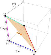
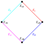
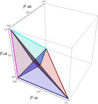
Figure 1: (Color online) Left: 3-dimensional phase space displaying the four families of equilibrium solutions: $E_{A}$ ($p_{aB}$ axis, purple), $E_{B}$ ($p_{Ab}$ axis, blue), $E_{a}$ (diagonal on the $p_{Ab}-p_{AB}$ plane, red) and $E_{b}$ (diagonal on the $p_{aB}-p_{AB}$ plane, cyan); $E_{ab}$, $E_{Ab}$, $E_{aB}$ and $E_{AB}$ (vertices connecting the first family, black circles); $EU_{1}$ and $EU_{2}$ (midpoints of edges of the phase space not containing the first family, orange circles); and $ES$ (center, brown circle). The shaded light brown surface represents the top face of the tetrahedral phase space of equation $p_{AB}+p_{Ab}+p_{aB}=1$. Middle: Schematic representation of the stable fixed points. Right: Division of the phase space displaying the basins of attraction of type 1 fixed points.

We start the discussion with type 3 fixed points for which the stability matrix is two times the identity. Therefore, it has one single fully degenerated eigenvalue $\zeta=2$ and both points $EU_{1}$ and $EU_{2}$ are unstable fixed points.

The stability matrix of $ES$ displays two different eigenvalues, $\zeta_{s}=2/3$ and $\zeta_{u}=4/3$, the latter with degeneration 2. Accordingly, this fixed point has a saddle like behavior, being unstable on a two dimensional subspace and stable on a one dimensional subspace. From a geometrical point of view, it is interesting to note that the points $EU_{1}$ and $EU_{2}$ are equidistantly located from $ES$ along the linear subspace spanned by the stable eigenvector ${\bf e}_{AB}-{\bf e}_{Ab}-{\bf e}_{aB}$ (Figure 1).

Fixed points of types 1 and 2 deserve a more detailed description. Not displaying exactly the same properties, they share common features, which makes instructive to analyze the stability of both types at the same time. We take as an example the set of points $E_{B}$, and its $\lambda_{B}\rightarrow 0$ and $\lambda_{B}\rightarrow 1$ limits, which are the points $E_{AB}$ and $E_{aB}$, respectively. Appendix C explains how to transfer the outcomes of the following analysis to the remaining type 1 and type 2 fixed points. The stability matrix for any of such points has the following eigenvalues and eigenvectors:

• $\zeta_{1}=\lambda_{B}$: ${\mathbf{v}_{1}}=\frac{1}{2}{\bf e}_{AB}-\lambda_{B}{\bf e}_{Ab}$.

• $\zeta_{2}=1-\lambda_{B}$: ${\mathbf{v}_{2}}=(\frac{1}{2}-\lambda_{B}){\bf e}_{Ab}+\frac{1}{2}{\bf e}_{aB}$.

• $\zeta_{3}=1$: ${\mathbf{v}_{3}}={\bf e}_{Ab}$.

In the first place, notice that along the direction spanned by ${\mathbf{v}_{3}}$ displacements are neutral. Indeed, since $\zeta_{3}=1$ for all points in the set, displacements from the fixed points in this direction are not amplified nor contracted. This is consistent with the fact that this direction corresponds to the $p_{Ab}$ axis itself, where the entire set $E_{B}$ is located. Therefore, by displacing a point from a fixed point in this direction one simply moves to another fixed point and thus iterations do not evolve it further.

In the directions spanned by ${\mathbf{v}_{1}}$ and ${\mathbf{v}_{2}}$, the eigenvalues show that the fixed points $E_{B}$ are stable (points $E_{AB}$ and $E_{aB}$ are also stable, however the stability can not be inferred from the eigenvalues). Notice that, properly scaled, eigenvectors ${\mathbf{v}_{1}}$ and ${\mathbf{v}_{2}}$ have the interesting property of connecting the fixed points $E_{B}$ (as well as $E_{AB}$ and $E_{aB}$) with the points $EU_{1}$ and $EU_{2}$, respectively. This property, illustrated in Figure 2, will be used in section IV.3.

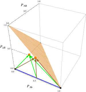
Figure 2: (Color online) Eigenvectors $\mathbf{v_{1}}$ (green) and $\mathbf{v_{2}}$ (brown) corresponding to the points $E_{B}$ (with $\lambda_{B}=1/2$), $E_{AB}$ and $E_{aB}$.

IV.2 Rates of convergence

Although the qualitative behavior of any fixed point in the set $E_{B}$ is the same (one neutral direction and two stable directions pointing to type 3 fixed points), and even for the extremes $E_{AB}$ and $E_{aB}$, points within the set differ from each other in the time to convergence. Close to the fixed points the movement along a given eigendirection obeys

$$x^{t+1}_{i}=\zeta_{i}x_{i},$$ (31)

so that

$$x_{i}=x_{i}^{0}\zeta_{i}^{t}\equiv x_{i}^{0}e^{-t/\tau_{i}},$$ (32)

($x_{i}^{0}$ being the i-th component of the initial displacement from the fixed point, for $i=1,2$) with

$$\tau_{i}=-\frac{1}{\ln{\zeta_{i}}}.$$ (33)

This allows to compare the time constants in the directions ${\mathbf{v}_{1}}$ and ${\mathbf{v}_{2}}$ as the parameter $\lambda_{B}$ varies along the set. The ratio gives

$$\frac{\tau_{1}}{\tau_{2}}=\frac{\ln{(1-\lambda_{B})}}{\ln{\lambda_{B}}}.$$ (34)

Accordingly, by displacing the fixed point close to the point $E_{AB}$ ($\lambda_{B}\sim 0$), the time of convergence along ${\mathbf{v}_{2}}$ becomes much larger compared to the time along ${\mathbf{v}_{1}}$. The opposite behavior is obtained by displacing the fixed point towards $E_{aB}$ ($\lambda_{B}\sim 1$).

For $\lambda_{B}$ strictly equal to zero, estimation (33) yields an infinitely slow convergence along ${\mathbf{v}_{2}}$, and an instantaneous convergence along ${\mathbf{v}_{1}}$. This is however a consequence of the attempt to linearize an equation with no linear contribution in its series expansion. Since $p_{Ab}=p_{aB}=0$ along ${\mathbf{v}_{1}}$, we can rewrite equation (27) as

$$p_{AB}^{t+1}=\frac{p_{AB}^{2}}{1-2p_{AB}(1-p_{AB})},$$ (35)

whose leading order is quadratic. We write therefore

$$p_{AB}^{t+1}=p_{AB}^{2}+O(p_{AB}^{3})$$ (36)

for points close to $E_{AB}$, whose leading order solution reads

$$p_{AB}=(p_{AB}^{0})^{2^{t}}.$$ (37)

Besides demonstrating stability, this solution shows that convergence is superfast in comparison to the exponential behavior for points $E_{B}$ (equation (32)).

In the ${\mathbf{v}_{2}}$ direction $p_{Ab}=p_{aB}$ and $p_{AB}=0$. Therefore, we rewrite equation (28) as

$$p_{Ab}^{t+1}=\frac{p_{Ab}(1-p_{Ab})}{1-2p_{Ab}^{2}}=p_{Ab}(1-p_{Ab})+O(p_{Ab}^{3}).$$ (38)

Even by neglecting the $O(p_{Ab}^{3})$ term, this equation does not have a closed solution foot1 . Yet, it is possible to extract a conclusion concerning stability and convergence rate. Successive iterations of equation (38) give

$$p_{Ab}=p_{Ab}^{0}\sum_{k=0}^{2^{t}-1}(-1)^{k}a_{k}(p_{Ab}^{0})^{k},$$ (39)

where $a_{0}=1$ and $a_{1}=t$. Accordingly, for times $t<O(1/p_{Ab}^{0})$ and points close to the fixed point along ${\mathbf{v}_{2}}$,

$$p_{Ab}\approx p_{Ab}^{0}(1-tp_{Ab}^{0})\approx\frac{p_{Ab}^{0}}{1+p_{Ab}^{0}t},$$ (40)

which again demonstrates stability, however a convergence results superslow when compared with points $E_{B}$. Numerical computations demonstrate that the right hand result is still valid for times arbitrarily large (see appendix D).

IV.3 Conserved quantities

Quantities not changing in time give powerful insights in the understanding of dynamical problems. In the absence of restrictions in reproduction, allele frequencies $\tilde{p}_{A}$ and $\tilde{p}_{B}$ remain constant and this property characterizes the equilibrium (20-23). Surprisingly, the dynamics under genetic restrictions has also a conserved quantity that, being different from the frequencies of the alleles, allows for a complete description of the dynamics and the equilibria.

Through equations (27-30) it can be shown that all allele frequencies obey the same evolution equation

$$\tilde{p}_{u}^{t+1}=\frac{\tilde{p}_{u}-1/2}{1-2\Delta}+1/2$$ (41)

for $u=A,B,a,b$. Writing this equation for $u=A$ and $u=B$ and dividing one by the other implies that the quantity

$$T=\frac{\tilde{p}_{A}-1/2}{\tilde{p}_{B}-1/2}$$ (42)

remains constant across generations. This implies that in the 3-dimensional haplotype phase space, the dynamics is constrained to the plane defined by the equation

$$p_{AB}+p_{Ab}-1/2-T(p_{AB}+p_{aB}-1/2)=0,$$ (43)

referred from now on as $T$-plane. Notice that the three aligned points $EU_{1}$, $EU_{2}$ and $ES$ are contained in the $T$-plane for any $T$. Changing the value of $T$ simply rotates the $T$-plane around the axis defined by these three points, making the description of the dynamics quite simple. Specifically, the location of the $T$-plane unambiguously determines two stable fixed points, which can be

1. $E_{B}$ and $E_{b}$ for $|T|<1$

2. $E_{A}$ and $E_{a}$ for $|T|>1$

3. $E_{AB}$ and $E_{ab}$ for $T=1$

4. $E_{Ab}$ and $E_{aB}$ for $T=-1$.

The stable eigenvectors ${\bf v}_{1}$ and ${\bf v}_{2}$, in turn, run along the borders of the $T$-plane. The dynamics reduces therefore to a 2-dimensional hyperbolic motion with the central fixed point $ES$ attracting trajectories in one direction (corresponding to the $EU_{1}-ES-EU_{2}$ axis) and repelling in the other direction. The latter, unstable direction, gives rise to the unstable manifold connecting $ES$ with two stable fixed points (in any of the four combinations listed above). Figure 3 illustrates the picture for $T=-0.8$.

From the previous paragraph results that by setting the plane of motion, initial conditions almost determine the equilibrium distribution of haplotype frequencies. There is still an ambiguity concerning which of the two stable fixed points intersected by the $T$-plane is attained. Of course, this ambiguity is solved by determining to which side respect to the the $EU_{1}-ES-EU_{2}$ axis the initial condition is located. As we demonstrate next, a simple algorithm to determine the latter issue consists in computing initial values of (10-13), and identifying the allele in the minor proportion.

The right panel of Figure 1 depicts a division of the haplotype space in four regions, and two planes forming the frontiers between them. These planes correspond to $T=1$, and $T=-1$. In terms of the alleles frequencies, a straightforward calculation shows that on the $(+1)$-plane $\tilde{p}_{A}=\tilde{p}_{B}$, whereas on the $(-1)$-plane $\tilde{p}_{A}+\tilde{p}_{B}=1$. Accordingly, in one and only one of the four regions, the alleles frequencies should satisfy

• $\tilde{p}_{A}<\tilde{p}_{B}$

• $\tilde{p}_{A}+\tilde{p}_{B}<1$

but the second relation implies $\tilde{p}_{A}<\tilde{p}_{b}$, which necessarily means $\tilde{p}_{A}<1/2$ and thus $\tilde{p}_{A}<\tilde{p}_{a}$. This region of the haplotype space is therefore characterized by the fact that the allele $A$ is the allele in the minor proportion. As type 1 fixed points labeled $E_{A}$ (in purple in Figure 1) have necessarily this property, it turns out that the region in consideration must contain all points in the phase space that are attracted to this set of fixed points. The conclusion is that points shadowed in light purple in Figure 1 are the points with allele A in the minor proportion, and evolve to fixed points $E_{A}$. Similar arguments allow to conclude that the light blue region contains initial conditions having allele $B$ in the minor proportion (evolving to fixed points $E_{B}$), light red region contains initial conditions with allele $a$ in the minor proportion (evolving to fixed points $E_{a}$), and finally, light cyan region contains initial conditions with allele $b$ in the minor proportion (evolving to fixed points $E_{b}$).

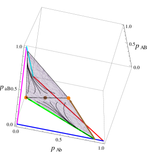
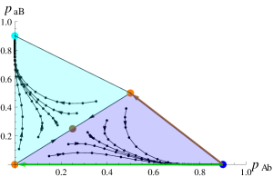
Figure 3: (Color online) Plane of motion corresponding to $T=-0.8$, and a set of trajectories with initial conditions chosen close to the stable manifold of $ES$. In the right pannel, a projection of the T-plane on the $p_{Ab}\!-\!p_{aB}$ plane. Arrows indicate the direction of motion, and shadowed regions represent the basins of attaction of fixed points $E_{b}$ (cyan) and $E_{B}$ (blue) (compare with figure 1). In green and brown, the eigenvectors of the equilibrium $E_{B}$. Notice the bending of the trajectories towards ${\bf v_{1}}$ (green vector), making evident the differential rates of convergence in the two eigendirections. In the picture $\lambda_{B}=0.9$, which corresponds to $\tau_{1}/\tau_{2}\approx 21.8$.

IV.4 Equilibrium

The construction presented above allows us to predict, for an arbitrary initial condition, the asymptotic equilibrium of the population in terms of two elements. First, it is necessary to establish the $T$-plane where the initial condition is located and, second, the allele in the smaller proportion. In the example of Figure 3, a bunch of trajectories is simulated taking initial conditions close to the $EU_{1}-ES-EU_{2}$ axis and having $T=-0.8$. The $T$-plane intersects the $E_{B}$ set for the initial conditions having $B$ in the smaller proportion and the $E_{b}$ set for initial conditions having $b$ in the smaller proportion. From the conservation of $T=-0.8$ results that at equilibrium the first bunch of trajectories converge to the point given by $\lambda_{B}=0.9$, and the second bunch of trajectories to the point given by $\lambda_{b}=0.1$.

The practical result of this analysis is that the smallest among the initial allelic frequencies always goes to zero. This information, together with the conserved quantity $T$ suffices to determine all frequencies. For example, if $p_{b}$ is the smallest initial frequency, in the equilibrium $p_{b}=0$ and, consequently, $p_{B}=1$. From equation (42) we find $p_{A}=(1+T)/2$ and $p_{a}=1-p_{A}=(1-T)/2$ and all haplotype frequencies have been calculated.

V Conclusions and biological implications

The procedure outlined in sections IV.3 and IV.4 to predict the equilibrium from the initial conditions, in addition to the information provided in section IV.2 concerning times to convergence, represent the full solution of the dynamics of the two-loci problem subjected to genetic restricted mating. Geometrically, the dynamics reduces to a foliation of the 3-dimensional haplotype space in planes with a very simple motion, consisting of a central hyperbolic point repelling trajectories towards two stable equilibria. Initial conditions and stable equilibria remain related through the existence of a conserved quantity $T$, which defines the planes where the hyperbolic motion takes place.

On the basis of times to convergence, stable equilibria can be divided in two categories. Stable equilibria of type 1 are attained exponentially, whereas type 2 equilibria are attained at much slower rates ($\delta^{t}=\frac{\delta^{0}}{1+\delta^{0}t}$, $\delta$ being the distance to the fixed point). It is interesting to observe that this classification has a biological counterpart. Specifically, slow-attained equilibria represent monomorphic populations, whereas exponentially-attained equilibria correspond to populations that are polymorphic at a single locus. Double-polymorphic populations are unstable (points of type 3 and 4) or evolve to any of the former scenarios, reveling the fact that genetic restricted mating has the net effect of a selection. As pointed out in Gavrilets (1999), models of incompatibility based on genetic distance have two alternative interpretations. One interpretation corresponds to sexual haploid populations with fitness assigned to pairs of individuals (here fitness is included in the rate $r_{h_{1}:h_{2}}$), and the second interpretation concerns diploid populations reproducing through random mating, where fitness is a function of individual heterozygosity. Accordingly, the model studied in this work describes an evolution process that eliminates double polymorphism (first interpretation) or alternatively a selection against double heterozigotes (second interpretation). Selection against heterozigote is also known as underdominance, and explains the disruptive selection causing sympatric speciation smith .

Section IV.3 revels another important aspect of restriction through genetic distance, which concerns the fact that the allele initially appearing in the smallest proportion remains always in the minor proportion, and vanish when the equilibrium is attained. The existence of the conserved quantity $T$, in turn, also has an interesting consequence from the biological point of view. As $\tilde{p}_{A}=1/2$ represents the maximum polymorphism at the first locus, $d_{A}=(\tilde{p}_{A}-1/2)^{2}$ can be interpreted as a measure of the monomorphism for that gene. Accordingly, the fact that $T^{2}=d_{A}/d_{B}$ remains constant along evolution, establishes that the correlation between the polymorphism at the two loci does not change.

In the general situation of $B$ genes and mating genetic restriction by a distance $G$, stable equilibria are expected to be of $G+1$ different types, in the form of full monomorphic populations, polymorphic populations at a single locus, polymorphic populations at only two loci, etc, up to polymorphic populations at the $G$ loci. Accordingly, such scenarios can be related to an elimination of $G\!+\!1$-uple to $B$-uple polymorphic populations, or alternatively as a selection against $G\!+\!1$-uple to $B$-uple heterozygotes. These results will be demonstrated in a subsequent publication. In a spatially structured population it might happen that different regions converge to different equilibria, resulting in reproductively isolated species as obtained in de_aguiar_global_2009 . As the case studied here exhibits reproductive isolation only in the trivial way accomplished by monomorphic species (for instance, populations $AB$ and $ab$ are isolated with genetic distance within the populations $d_{w}=0$), it is of special interest to explicitly consider the case $B=3$ and $G=1$. In this situation, populations $ABC\!-\!ABc$ and $abC\!-\!abc$ are reproductively isolated with $0<d_{w}<1$. Moreover, the existence of a third single polymorphic species $ABc\!-\!Abc$, or even the monomorphic species $Abc$, may create an ring structure, revealing the richness of scenarios that can be realized through this simple arrangement. From the analysis of the times to convergence of section IV.2, it is also expected that times to convergence for $G=1$ will behave in the same way even for $B>2$, displaying an exponential behavior for single polymorphic species, and a superslow convergence for monomorphic species. These times to convergence should eventually be compared with the time to fixation driven by random drift. As the model studied here assumes infinite size populations, the model should be modified to take finite populations into account. A possible way to estimate the time to fixation driven by random drift would be a Moran approach moran ; moranaguiar . The case $B=3$ and $G=2$, on the other hand, represents also an interesting issue to investigate, as it is expected to display three different time scales of convergence, corresponding to three types of stable equilibria.

The scenarios described in the previous paragraph, as well as the influences of mutations on the results of section IV, will be the subject of a future work. Nevertheless, we stress the importance of the study accomplished so far, as it reveals aspects of the dynamics that necessarily help to undertake the analysis in more complex frameworks.

Acknowledgments. We thank Yaneer Bar-Yam for helpful comments and discussions. This work was partly supported by FAPESP (Fundação de Amparo à Pesquisa do Estado de São Paulo) and CNPq (Conselho Nacional de Desenvolvimento Científico e Tecnológico).

Appendix A Evolution of the haplotypic frequencies under random mating

In this appendix we solve equations (6-9), performing explicit calculations for the expression (6). The remaining solutions can be obtained in an equivalent way. We write explicitly the time dependence

$$p_{AB}^{t+1}=p_{AB}^{t}-\frac{1}{2}D^{t},$$ (44)

or

$$p_{AB}^{1} = p_{AB}^{0}-\frac{1}{2}D^{0}$$

$$p_{AB}^{2} = p_{AB}^{0}-\frac{1}{2}D^{1}-\frac{1}{2}D^{0}$$

$$p_{AB}^{3} = p_{AB}^{0}-\frac{1}{2}D^{2}-\frac{1}{2}D^{1}-\frac{1}{2}D^{0}$$

$$\vdots$$

$$p_{AB}^{t} = p_{AB}^{0}-\frac{1}{2}\displaystyle\sum_{i=0}^{t-1}D^{i}.$$ (45)

On the other hand, using the result (15) yields

$$p_{AB}^{t}=p_{AB}^{0}-\frac{D^{0}}{2}\displaystyle\sum_{i=0}^{t-1}2^{-i}=p_{AB}^{0}-D^{0}(1-2^{-t}),$$ (46)

For long times, we obtain the equilibrium solutions,

$$p_{AB}^{\rm eq} = p_{AB}^{0}-D^{0}$$

$$p_{bB}^{\rm eq} = p_{Ab}^{0}+D^{0}$$

$$p_{aB}^{\rm eq} = p_{aB}^{0}+D^{0}$$

$$p_{ab}^{\rm eq} = p_{ab}^{0}-D^{0}.$$ (47)

Appendix B Relationship between allele and haplotype frequencies

Here we demonstrate the product relationship between the allele and the haplotype frequencies when mating is not restricted by genetic distance. Given the definitions of the allele frequencies, we calculate, for instance, the product $\tilde{p}_{A}\tilde{p}_{B}$

$$\tilde{p}_{A}\tilde{p}_{B} = (p_{AB}+p_{Ab})(p_{AB}+p_{aB})$$ (48)

$$= p_{AB}(p_{AB}+p_{Ab}+p_{aB})+p_{Ab}p_{aB}$$

$$= p_{AB}(1-p_{ab})+p_{Ab}p_{aB}$$

$$= p_{AB}-D.$$

Using the result (15) leads to

$$p_{AB}=\tilde{p}_{A}\tilde{p}_{B}+\frac{D^{0}}{2^{t}}.$$ (49)

The equilibrium corresponds to the asymptotic limit of the previous equation, and is approached after a small number of generations

$$p_{AB}^{\rm eq}=\tilde{p}_{A}\tilde{p}_{B}.$$ (50)

Strictly speaking, $|p_{AB}-\tilde{p}_{A}\tilde{p}_{B}|<1\%$ of the equilibrium value $\tilde{p}_{A}\tilde{p}_{B}$ in less than ten generations.

Appendix C Stability of fixed points of type 1 and 2 (complement)

In this appendix we extend the results of the stability analysis of section IV.1 for the fixed points $E_{A}$, $E_{B}$ and $E_{b}$. We start with the eigenvalues and eigenvectors of the stability matrices of the different fixed points.

Stability of points $E_{A}$ (purpple line, $p_{aB}=\lambda_{A})$

• $\zeta_{1}=\lambda_{A}$: $\quad\qquad{\mathbf{v}_{1}}=\frac{1}{2}{\bf e}_{Ab}-\lambda_{A}{\bf e}_{aB}$

• $\zeta_{2}=1-\lambda_{A}$: $\quad{\mathbf{v}_{2}}=\frac{1}{2}{\bf e}_{Ab}+(\frac{1}{2}-\lambda_{a}){\bf e}_{aB}$.

• $\zeta_{3}=1$: $\quad\qquad{\mathbf{v}_{3}}={\bf e}_{aB}$.

Stability of points $E_{a}$ (red line, $p_{AB}=\lambda_{a}$, $p_{Ab}=1-\lambda_{a}$)

• $\zeta_{1}=1-\lambda_{a}$: $\quad{\mathbf{v}_{1}}=(\frac{1}{2}-\lambda_{a}){\bf e}_{AB}+(-1+\lambda_{a}){\bf e}_{Ab}$.

• $\zeta_{2}=\lambda_{a}$: $\quad\qquad{\mathbf{v}_{2}}=-\lambda_{a}{\bf e}_{AB}+(-\frac{1}{2}+\lambda_{a}){\bf e}_{Ab}+{\bf e}_{aB}$

• $\zeta_{3}=1$: $\quad\qquad{\mathbf{v}_{3}}={\bf e}_{AB}-{\bf e}_{Ab}$.

Stability of points $E_{b}$ (cyan line, $p_{AB}=\lambda_{b}$, $p_{aB}=1-\lambda_{b}$)

• $\zeta_{1}=1-\lambda_{b}$: $\quad{\mathbf{v}_{1}}=(\frac{1}{2}-\lambda_{b}){\bf e}_{AB}-(1-\lambda_{b}){\bf e}_{aB}$.

• $\zeta_{2}=\lambda_{b}$: $\quad\qquad{\mathbf{v}_{2}}=-\lambda_{b}{\bf e}_{AB}+{\bf e}_{Ab}+(-\frac{1}{2}+\lambda_{b}){\bf e}_{aB}$

• $\zeta_{3}=1$: $\quad\qquad{\mathbf{v}_{3}}=-{\bf e}_{AB}+{\bf e}_{aB}$.

Stable eigenvectors corresponding to points of type 1 and type 2, properly scaled, connect the fixed points with type 3 fixed points. In Figure 4 we expose this important property for some specific points at each set, including the points $E_{B}$ analyzed in section IV.1.

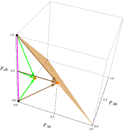
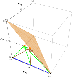
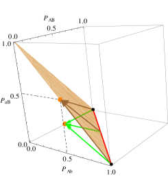
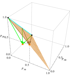
Figure 4: (Color online) Eigenvectors corresponding to type 1 and type 2 fixed points (vectors ${\mathbf{v}_{1}}$ in green, and ${\mathbf{v}_{2}}$ in brown).

Rates of convergence are inferred from the relation

$$\tau_{i}=-\frac{1}{\ln{\zeta_{i}}}$$ (51)

where $i=1,2$ denotes the type 3 fixed point ($EU_{1}$ or $EU_{2}$) to which the eigenvector points. Accordingly, going through the set $E_{a}$ from $E_{aB}$ to $E_{ab}$ (see Figure 5), makes $\tau_{1}$ to decreases. This time becomes almost zero at the point $E_{ab}$ (superfast convergence), and it starts increasing again by going to $E_{Ab}$ through the set $E_{b}$ (cyan line in Figure 5). At this $\tau_{1}$ becomes infinite (superslow convergence), which means an equivalent behavior to that corresponding to $E_{Ab}$. On the other hand, as $\zeta_{2}=1-\zeta_{1}$, it turns out that $\tau_{2}$, the time to convergence along the directions spanned by ${\mathbf{v_{2}}}$, displays the opposite behavior. Finally, the picture is completed by observing that the remaining branch of the cycle ($E_{Ab}\rightarrow E_{AB}$ along $E_{A}$ and $E_{AB}\rightarrow E_{aB}$ along $E_{B}$) is an exact repetition of the branch described above.

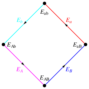
Figure 5: (Color online) Schematic representation of type 1 and type 2 fixed points. Arrows indicate the direction of the walk employed in the text to describe the behavior of the rates of convergence.

Appendix D Numerical solution of equation (38)

Here we give a brief summary of the fitting process employed to solve equation (38). By iterating the map for different initial conditions and fitting the results, one obtains

$$p_{Ab}^{t}=\frac{1}{A(p_{Ab}^{0})+t},$$ (52)

where $A(x)$ is a function that diverges as $1/x$ when $x\rightarrow 0$ (see Figure 6). Accordingly, for very small $p_{Ab}^{0}$ values we can write

$$p_{Ab}^{t}=\frac{p_{Ab}^{0}}{1+p_{Ab}^{0}t}+O((p_{Ab}^{0})^{2}).$$ (53)

(a) (Color online) Iterations of the map for the initial condition $p_{Ab}^{0}=0.1$. The fitting gives $1/p_{Ab}=12.336+1.002t$.

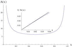
(b) (Color online) Plot of the function $A(x)$ (see the text). In the inset we plot $1/A(x)$ to demonstrate that, for very small $x$ values $1/A(x)=x+O(x^{2})$ (black curve: $f(x)=x)$.

Figure 6: Fitting results related to the eigenvector $\mathbf{v}_{2}$ of the stability matrix associated to $E_{AB}$.

References

- Coyne and Orr (2004) J.A Coyne and H.A. Orr, 2004. Speciation. 1 ed. Sinauer Associates, Inc.
- (2) S. Gavrilets, 2004. Fitness Landscapes and the Origin of Species (MPB-41). Princeton University Press.
- Butlin et al. (2012) R.A. Butlin et al., Trends Ecol. Evol. 27 (2012) 27.
- Nosil (2012) P. Nosil, 2012. Ecological speciation. Oxford University Press, Oxford; New York.
- (5) P.G. Higgs and B.Derrida, J. Phys. A. 24, L985 (1991).
- (6) P.G. Higgs and B.Derrida, J. Mol. Evol. 35, 454 (1992).
- (7) A.S. Kondrashov, M. Shpak, Proc. Soc. Lond R 265 (1998) 2273.
- Dieckmann and Doebeli (1999) U. Dieckmann, M. Doebeli, Nature 400 (1999) 354.
- Gavrilets (1999) S. Gavrilets, The Am. Natur. 154 (1999) 1.
- (10) G.A. Hoelzer, R. Drewes, J. Meier and R. Doursat, PLoS Comput. Biol. 4 e1000126 (2008).
- Doorn et al. (2009) G.S. v. Doorn, P. Edelaar, and F.J. Weissing, Science 326 (2009) 1704.
- (12) B.M. Fitzpatrick, J.A. Fordyce, S. Gavrilets, J. Evol. Biol. 22 (2009) 2342.
- (13) de Aguiar, M.A.M., M. Baranger, E.M. Baptestini, L. Kaufman, and Y. Bar-Yam, Nature 460 (2009) 384
- (14) D. Ashlock, E.L. Clare, T.E. von Konigslow, W. Ashlock, J. Theor. Biol. 264 (2010) 1202.
- (15) M. Kopp, BioEssays 32 (2010) 564.
- (16) C. J. Melian, C. Vilas, F. Baldo, E. Gonzalez-Ortegon, P. Drake and R. J. Williams, Ad. Ecol. Res. 45 (2011) 225.
- (17) P. Desjardins-Proulx, D. Gravel, The Am. Natur. 179 (2012) 137
- Martins et al. (2013) A.B. Martins, M.A.M. de Aguiar, and Y. Bar-Yam, PNAS 110 (2013) 5080.
- Gavrilets et al. (2000) S. Gavrilets, H. Li, M.D. Vose, Proc. Biol. Sci. 54 (2000) 1126.
- Candolin (2003) U. Candolin, Biological Reviews 78 (2003) 575.
- (21) E.M. Baptestini, M.A.M. de Aguiar, Y. Bar-Yam, J. Theor. Biol. 335 (2013) 51.
- (22) D.M. Schneider, E. do Carmo, Y. Bar-Yam, M.A.M. de Aguiar, Phys. Rev. E 86 (2012) 041104.
- (23) J.F Crow and M. Kimura, 1970. An Introduction to Population Genetics Theory, The Blackburn Press.
- (24) W.J. Ewens Mathematical Population Genetics I. Theoretical Introduction Series: Biomathematics, Vol. 9 (New York: Springer Verlag, 1979).
- (25) P.A.P. Moran, Proc. Cam. Phil. Soc. 54 60 (1958).
- (26) M.A.M. de Aguiar and Y. Bar-Yam, Phys. Rev. E 84 (2011) 031901.
- (27) The equation is a particular case of the logistic map , having analytical solutions only for , and .
- (28) J. M. Smith, The Am. Natur. 100 (1966) 637.