Truncated hierarchical preconditioning for the stochastic Galerkin FEM

Abstract

Stochastic Galerkin finite element discretizations of partial differential equations with coefficients characterized by arbitrary distributions lead, in general, to fully block dense linear systems. We propose two novel strategies for constructing preconditioners for these systems to be used with Krylov subspace iterative solvers. In particular, we present a variation on of the hierarchical Schur complement preconditioner, developed recently by the authors, and an adaptation of the symmetric block Gauss-Seidel method. Both preconditioners take advantage of the hierarchical structure of global stochastic Galerkin matrices, and also, when applicable, of the decay of the norms of the stiffness matrices obtained from the polynomial chaos expansion of the coefficients. This decay allows to truncate the matrix-vector multiplications in the action of the preconditioners. Also, throughout the global matrix hierarchy, we approximate solves with certain submatrices by the associated diagonal block solves. The preconditioners thus require only a limited number of stiffness matrices obtained from the polynomial chaos expansion of the coefficients, and a preconditioner for the diagonal blocks of the global matrix. The performance is illustrated by numerical experiments.

1 Introduction

Precise values of coefficients in the setup of physical models using partial differential equations (PDEs) are often not known. In such situations, the coefficients are typically treated as random variables or processes in attempt to quantify uncertainty in the underlying problem. Probably the most popular and widely used class of methods for a solution of these problems are the Monte-Carlo techniques, because they require only solutions of the PDE for a given set of realizations of the input random coefficients. These methods are well-known for their robustness, versatility, and quite slow convergence. Therefore, in the last two decades, a significant effort has been devoted to the development of methods that leverage regularity of the solution, and outperform the Monte-Carlo methods at least for problems with stochastic dimensions that are not too large. The most promising developments include the stochastic finite element methods. There are two main variants of the stochastic finite elements: collocation methods [1, 2], and stochastic Galerkin methods [3, 4, 5]. The first approach samples the stochastic PDE at a predetermined set of collocation points, which yields a set of uncoupled deterministic systems. The solution at these collocation points is then used to interpolate the solution in the entire random input domain. Because extending legacy software to support the collocation points is relatively simple, these methods are often regarded as non-intrusive. On the other hand, the second approach, using the stochastic Galerkin methods, translates the stochastic PDE into one large coupled deterministic system. Consequently, the Galerkin methods require a development of new solvers and therefore they are commonly regarded as intrusive. Since use of direct solvers for the stochastic Galerkin systems might be prohibitive due to their large size, iterative solvers are often preferred. We then seek preconditioners to speed up convergence.

There are two main types of expansion of the random field representing the uncertainty in the coefficients of the underlying model. The first one, known as Karhunen-Loève (KL) expansion [6], is suitable for a finite-dimensional representation of Gaussian random fields, and leads in conjunction with the stochastic Galerkin finite element discretizations to block sparse structure of global matrices. Random fields with general probability distributions are also sometimes represented using the KL expansion, however it might be more suitable to use so-called generalized polynomial chaos (gPC) expansion [7] for their representation. This in general leads to block dense structure of the global matrices. In particular, in this paper we will focus on the random coefficients of the model elliptic PDE with lognormal distribution. Such discretization is done within the gPC framework, using Hermite polynomials [8]. It has been shown in [9, Theorem 18] that in order to guarantee a complete representation of the lognormal random field, one has to use twice the order of polynomial expansion of the coefficient than of the solution, which indeed leads to a fully block dense structure of the global stochastic Galerkin matrix. Clearly, based on the block sparsity pattern of the global stochastic Galerkin matrix, a certain class of preconditioners might be more suitable, compared to the others, for a particular problem to be solved.

Probably the most simple, yet quite powerful method is the mean-based preconditioner proposed by Pellissetti and Ghanem [10] and analyzed by Powell and Elman [11]. It is a block diagonal preconditioner which uses the information carried by the mean of the random coefficient and the corresponding stiffness matrix, i.e., the zeroth order term of the coefficient expansion. Subsequently, Ullmann has developed a Kronecker product preconditioner [12], cf. also [13], that makes use of information carried by higher order terms and improves the convergence quite significantly. The preconditioner has the Kronecker product structure of the global stochastic Galerkin matrix. Various iterative methods and preconditioners including multigrid methods, based on matrix splitting, were compared by Rosseel and Vandewalle in [14]. Most recently, the authors have developed in [15] a hierarchical Schur complement preconditioner that takes advantage of the recursive hierarchy in the structure of the global stochastic Galerkin matrix. We note that an interesting approach to solver parallelization has been proposed by Keese and Matthies [16], and a block-triangular preconditioner for the block sparse case has been proposed recently by Zheng et al. [17]. Finally, we refer to Ernst and Ullmann [18] for a more general study of the stochastic Galerkin matrices.

In this paper, we propose two novel strategies for constructing preconditioners for solution of the linear systems with block dense global matrices to be used with Krylov subspace iterative methods. In particular, we present a variation on the hierarchical Schur complement preconditioner developed recently by the authors [15], and an adaptation of the symmetric block Gauss-Seidel method. Both preconditioners are built in a way to account for the recursive hierarchy in the structure of the global stochastic Galerkin matrix. Because, unlike in the block sparse case, neither of the submatrices in this hierarchy is block diagonal, we approximate solves with submatrices by the associated diagonal block solves. This variant yields versions of the two preconditioners, which will be called as approximate. We note that the approximate versions thus use “locally” the block diagonal preconditioning, which allows for a certain level of decoupling. Our numerical experiments indicate that this approximation might not be necessarily traded off for slower convergence rates. In the second variation, we take take an advantage of the decay of the norms of the stiffness matrices obtained from the polynomial chaos expansion of the coefficients. The decay of the matrices allows to truncate the matrix-vector multiplications in the action of the preconditioners, and therefore these versions of the preconditioners will be called as truncated. We also note that one can replace the direct solvers of the diagonal blocks by iterative ones, possibly with the same tolerance as for the outer iterations. Doing so, the preconditioners become variable and one has to make a careful choice of the Krylov iterative method used for the global (outer) iterations. In general, it is recommended to use flexible methods such as the flexible conjugate gradients [19], FGMRES [20], or GMRESR [21]. Thus neither the global matrix, nor the matrix of the preconditioner need to be formed explicitly, and we can use the so called MAT-VEC operations introduced in [10] for all matrix-vector multiplications. Provided that we have a preconditioner for the diagonal block solves available, the ingredients of our methods include only the number of stiffness matrices from the expansion of the random coefficient. Therefore, the proposed methods can be viewed as minimally intrusive because they can be built as wrappers around existing solvers for the corresponding deterministic problem. Finally, we note that choice of a preconditioner for the diagonal block solves would not change the convergence in terms of outer iterations, and we will address this topic elsewhere.

The paper is organized as follows. In Section 2 we introduce the model problem and its discretization, in Section 3 we discuss the structure of the stochastic Galerkin matrices, in Section 4 we formulate our algorithms, in Section 5 we present some numerical experiments, and finaly in Section 6 we summarize and conclude our work.

2 Model problem

Let $\left(\Omega,\mathcal{F},\mu\right)$ denote the probability space associated with a physical experiment. We are interested in the solution of the stochastic linear elliptic boundary value problem, with stochastic input and deterministic data, given in a bounded domain$~{}D\subset$ $\mathbb{R}^{d}$, $d=2,3$. The solution is a random function$~{}u\left(x,\omega\right):\overline{D}\times\Omega\rightarrow\mathbb{R}$ that almost surely (a.s.) satisfies the equation

$$-\nabla\cdot\left(k\left(x,\omega\right)\,\nabla u\left(x,\omega\right)\right) =f\left(x\right)\qquad\text{in}\ D\times\Omega,$$ (1)

$$u\left(x,\omega\right) =0\qquad\text{on}\ \partial D\times\Omega,$$ (2)

where $f\in L^{2}\left(D\right)$, the gradient symbol $\nabla$ denoting the differentiation with respect to the spatial variables, and

$$0<k_{\min}\leq k\left(x,\omega\right)\qquad\text{a.s. in }\Omega,\;\forall x\in\overline{D}.$$

The function$~{}k\left(x,\omega\right):$ $\overline{D}\times\Omega\rightarrow\mathbb{R}$ is a random scalar field with a continuous and square-integrable covariance function. We will assume that the randomness of $k\left(x,\omega\right)$ is induced by a set of random variables $\xi\left(\omega\right)=\left\{\xi\left(\omega\right)\right\}_{i=1}^{N}$ that are assumed to be independent Gaussian with zero mean and unit variance. Thus the domain of $k\left(\cdot,\omega\right)$ is restricted to the subset $\left(\Omega,\mathcal{F}\left(\mathcal{\xi}\right),\mu\right)$ of $\left(\Omega,\mathcal{F},\mu\right)$ where $\mathcal{F}\left(\xi\right)$ is the $\sigma-$algebra generated by $\xi$. We will henceforth use $k\left(x,\xi\right)$ instead of  $k\left(x,\omega\right)$, and the solution $u\left(x,\omega\right)$ can be also written as $u\left(x,\xi\right)$.

In the variational formulation of problem (1)-(2), we consider the solution of the equation

$$u\in U:\ a\left(u,v\right)=\left\langle f,v\right\rangle,\qquad\forall v\in U.$$ (3)

where $U$ is a tensor product space defined as

$$U=H_{0}^{1}\left(D\right)\otimes L^{2}\left(\Omega\right),\qquad\left\|u\right\|_{U}=\sqrt{\mathbb{E}\left[\int_{D}\left|\nabla u\right|^{2}dx\right]},$$

where $\mathbb{E}\left[\cdot\right]$ denotes mathematical expectation, and the bilinear form $a\left(\cdot,\cdot\right)$ along with the right-hand side are defined as

$$a\left(u,v\right)=\mathbb{E}\left[\int_{D}k\left(x,\xi\right)\,\nabla u\cdot\nabla v\,dx\right],\qquad\left\langle f,v\right\rangle=\mathbb{E}\left[\int_{D}f\,v\,dx\right].$$

We assume that $k\left(x,\xi\right)$ can be represented, using a generalized polynomial chaos (gPC) expansion, as

$$k\left(x,\xi\right)=\sum_{i=0}^{M^{\prime}}k_{i}\left(x\right)\psi_{i}\left(\xi\right),\quad\text{where }k_{i}\left(x\right)=\frac{\mathbb{E}\left[k\left(x\right)\psi_{i}\left(\xi\right)\right]}{\mathbb{E}\left[\psi_{i}^{2}\right]},$$ (4)

and $\left\{\psi_{i}\left(\xi\right)\right\}_{i=0}^{M^{\prime}}$ is a set of $N-$dimensional Hermite polynomials [5]. Similarly, we will look for an expansion of the solution as

$$u\left(x,\xi\right)=\sum_{i=0}^{M}u_{i}\left(x\right)\psi_{i}\left(\xi\right),$$ (5)

that converges in $L^{2}\left(\Omega\times D\right)$ as $M\rightarrow\infty$. We will, in particular, model $k\left(x,\xi\right)$ as a truncated lognormal process. To this end, let $g\left(x,\xi\right)=g_{0}\left(x\right)+\sum_{i=1}^{N}\xi_{i}g_{i}\left(x\right)$ be a truncated Karhunen-Loève expansion of a Gaussian process defined on$~{}D$ with known mean $g_{0}\left(x\right)$ and covariance function$~{}C_{g}\left(x,y\right)$, i.e., $g_{i}\left(x\right)$ are weighted eigenfunctions of

$$\int_{D}C_{g}\left(x,y\right)\varphi_{i}\left(y\right)\,dy=\lambda_{i}\varphi_{i}\left(x\right),\quad\forall x\in D,\qquad\text{and\quad}g_{i}\left(x\right)=\sqrt{\lambda_{i}}\varphi_{i}\left(x\right)\text{.}$$ (6)

Then $k\left(x,\xi\right)$ is defined as $k\left(x,\xi\right)=\exp\left[g\left(x,\xi\right)\right]$. The procedure for computing the coefficients $k_{i}\left(x\right)$ in (4) has been derived by Ghanem in [8]. Denoting $\eta_{j}=\xi_{j}-g_{j}$, the coefficients are precisely given, cf. [8, eq. (33)], as

$$k_{i}\left(x\right)=\frac{\mathbb{E}\left[\psi_{i}\left(\eta\right)\right]}{\mathbb{E}\left[\psi_{i}^{2}\right]}\exp\left[g_{0}\left(x\right)+\frac{1}{2}\sum_{j=1}^{N}\left(g_{j}\left(x\right)\right)^{2}\right].$$ (7)

According to [9], in order for (4) to guarantee a complete representation of the lognormal random field, the order of polynomial expansion of$~{}k\left(x,\xi\right)$ in (4) should be twice the order of the expansion of the solution$~{}u\left(x,\xi\right)$ in (5). Denoting the two orders of the polynomial expansions of $u\left(x,\xi\right)$ and $k\left(x,\xi\right)$ as $P$ and $P^{\prime}$, resp., with $P^{\prime}=2P$, the total numbers of the gPC polynomials are

$$M+1=\frac{\left(N+P\right)!}{N!P!},\quad M^{\prime}+1=\frac{\left(N+P^{\prime}\right)!}{N!P^{\prime}!}=\frac{\left(N+2P\right)!}{N!\left(2P\right)!}.$$ (8)

We will consider approximations to the variational problem (3) given by the finite element discretizations of$~{}H_{0}^{1}\left(D\right)$. The solution$~{}u\left(x,\xi\right)$ from (5) will be thus approximated by

$$u\left(x,\xi\right)=\sum_{i=1}^{N_{\text{dof}}}\sum_{j=0}^{M}u_{ij}\phi_{i}\left(x\right)\psi_{j}\left(\xi\right),$$ (9)

where $\left\{\phi_{i}\left(x\right)\right\}_{i=1}^{N_{\text{dof}}}$ is a finite element basis, and $\left\{\psi_{j}\left(\xi\right)\right\}_{j=0}^{M}$ is the basis of the Hermite polynomials described above. Substituting the expansions (4) and (9) into (3) yields a deterministic system of linear equations

$$\sum_{j=0}^{M}\sum_{i=0}^{M^{\prime}}c_{ijk}K_{i}u_{j}=f_{k},\qquad k=0,\dots,M,$$ (10)

where $(f_{k})_{l}=\mathbb{E}\left[\int_{D}f\left(x\right)\phi_{l}\left(x\right)\psi_{k}\,dx\right]$, $\left(K_{i}\right)_{lm}=\int_{D}k_{i}(x)\phi_{l}(x),\phi_{m}(x)\,dx$, and $c_{ijk}=\mathbb{E}\left[\psi_{i}\psi_{j}\psi_{k}\right]$. Each one of the blocks $K_{i}$ is thus a deterministic stiffness matrix given by$~{}k_{i}\left(x\right)$ of size $N_{\text{dof}}\times N_{\text{dof}}$, where $N_{\text{dof}}$ is the number of spatial degrees of freedom. The system (10) is given by a global stochastic Galerkin matrix of size $\left(M+1\right)N_{\text{dof}}\times\left(M+1\right)N_{\text{dof}}$, consisting of $N_{\text{dof}}\times N_{\text{dof}}$ blocks $K^{\left(j,k\right)}$, and it can be written as

$$\left[\begin{array}[c]{ccccc}K^{\left(0,0\right)}&K^{\left(0,1\right)}&\cdots&&K^{\left(0,M\right)}\\ &\ddots&&&\\ \vdots&&K^{\left(k,k\right)}&&\vdots\\ &&&\ddots&\\ K^{\left(M,0\right)}&K^{\left(M,1\right)}&\cdots&&K^{\left(M,M\right)}\end{array}\right]\left[\begin{array}[c]{c}u_{\left(0\right)}\\ \vdots\\ u_{\left(k\right)}\\ \vdots\\ u_{\left(M\right)}\end{array}\right]=\left[\begin{array}[c]{c}f_{\left(0\right)}\\ \vdots\\ f_{\left(k\right)}\\ \vdots\\ f_{\left(M\right)}\end{array}\right],$$ (11)

where each of the blocks $K^{\left(j,k\right)}$ is obtained as

$$K^{\left(j,k\right)}=\sum_{i=0}^{M^{\prime}}c_{ijk}K_{i}.$$ (12)

We note that the first diagonal block is obtained by the $0-$th order polynomial chaos expansion and therefore corresponds to the deterministic problem obtained using the mean value of the coefficient$~{}k_{0}$. In particular,

$$K^{\left(0,0\right)}=K_{0}.$$

In the next section we discuss the structure of the global stochastic Galerkin matrix from (11) in somewhat more detail.

3 Hierarchical structure of the matrices

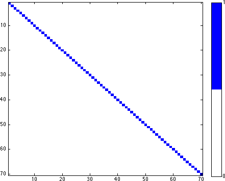
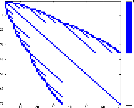
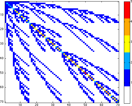
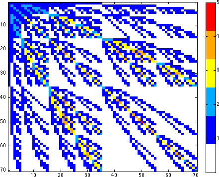
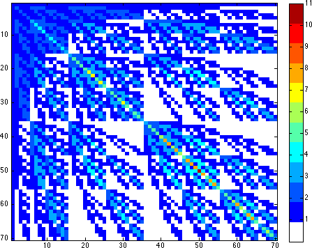
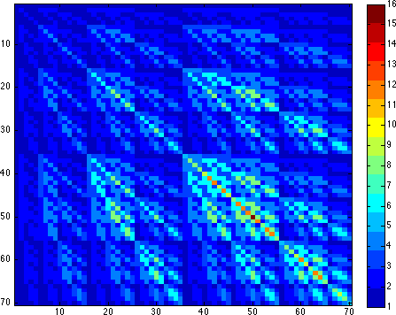
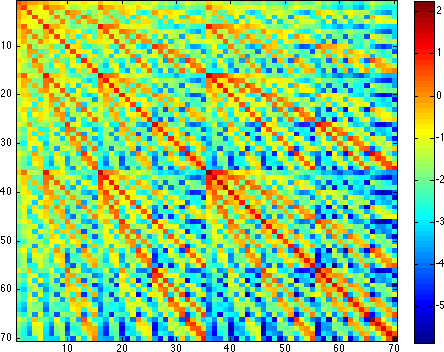
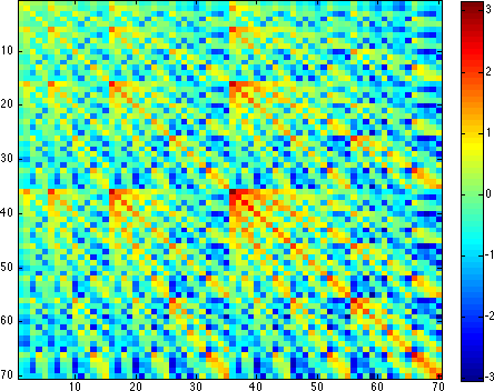
The stochastic Galerkin matrices have recently received quite a lot of attention, cf., e.g., [18, 9, 14]. The key role in their block structure is played by the constants $c_{ijk}$ and the upper bound of the summation in equation (12). In general, there are two types of block sparsity patterns. The first type, typically regarded as block sparse, is associated with use of only the linear terms $\xi_{1},\dots,\xi_{N}$ such as appearing in a Karhunen-Loève expansion of $k\left(x,\xi\right)$, cf. Figure 1(b). The second type, block dense, is associated with a general (nonlinear in $\xi$’s) form of the expansion as in (4). We note that due to our setup with $P^{\prime}=2P$, we obtain that $M^{\prime}\gg M$ from (8), and the matrices are in general fully dense, cf. Figure 1(f). Recently, we proposed a preconditioner suitable for iterative solution of block sparse stochastic Galerkin systems [15]. Here, we will focus on a design of preconditioners for more general, block dense, linear systems.

The structure of the global stochastic Galerkin matrix can be understood through knowledge of the coefficient matrix$~{}c_{P}$ with entries $c_{P}\left(j,k\right)=\sum_{i=0}^{M^{\prime}}c_{ijk}$ where $j,k=0,\dots,M$, and the value of$~{}M$ follows from the fact that we use the $P-$th order polynomial expansion, cf. (8)  In general, let us consider some $\ell-$th order polynomial expansion, such that$\ 1\leq\ell\leq P.$ It is easy to see that the corresponding coefficient matrix$~{}c_{\ell}$ will have a hierarchical structure

$$c_{\ell}=\left[\begin{array}[c]{cc}c_{\ell-1}&b_{\ell}^{T}\\ b_{\ell}&d_{\ell}\end{array}\right],\qquad\ell=1,\dots,P,$$ (13)

where $c_{\ell-1}$ are the first principal submatrices corresponding to the the $\left(\ell-1\right)-$th order polynomials expansion. We note that even though the matrices $c_{\ell}$ are symmetric, the global stochastic Galerkin matrix in (11) will be symmetric only if each one of the stiffness matrices $K_{i}$ is symmetric. Clearly, all matrices $K_{i}$ will have the same sparsity pattern.

In either case, the block sparse or the block dense, the linear system (11) can be written as

$$A_{P}u_{P}=f_{P},$$ (14)

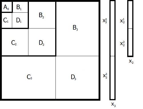
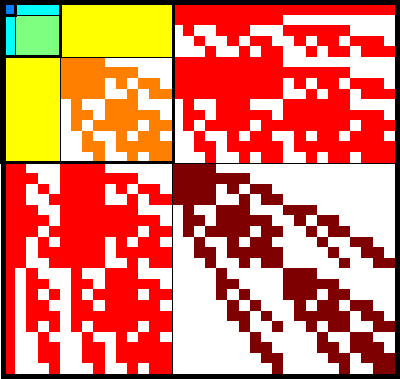
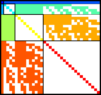
where the global Galerkin matrix $A_{P}$ has the hierarchical structure, cf. Figure 2(a), given as

$$A_{\ell}=\left[\begin{array}[c]{cc}A_{\ell-1}&B_{\ell}\\ C_{\ell}&D_{\ell}\end{array}\right],\qquad\ell=P,\dots,1,$$ (15)

and $A_{0}=K_{0}$ is the matrix of the mean. Although for the model problem (1)-(2) it holds that $C_{\ell}=B_{\ell}^{T}$, for$~{}\ell=1,\dots P$, we will use the general notation of (15) for the sake of generality.

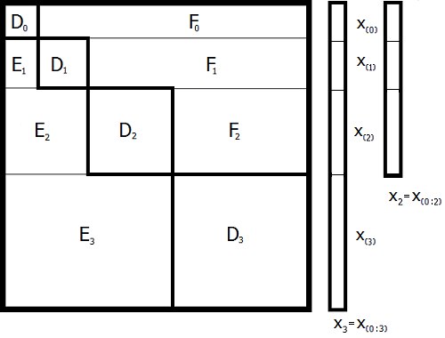
Alternatively, let us consider a hierarchical splitting of the matrix$~{}A_{P}$, cf. Figure 2(b), as

$$A_{P}=\left[\begin{array}[c]{ccccccc}D_{0}&&&&F_{0}&&\\ &\ddots&&&&&\\ &&\ddots&&&&\\ &E_{\ell}&&D_{\ell}&&F_{\ell}&\\ &&&&\ddots&&\\ &&&&&\ddots&\\ &&E_{P}&&&&D_{P}\end{array}\right].$$ (16)

The blocks $D_{\ell}$, $\ell=1,\dots,P$, are the same in (15) and (16), and we have also, for convenience, denoted $D_{0}=A_{0}$.

The decomposition (15) has served as a starting point for the hierarchical Schur complement preconditioner in [15], and we will use the decomposition (16) to formulate the hierarchical block symmetric Gauss-Seidel preconditioner. Since we are interested here only in the preconditioners that are block and symmetric we will drop the two words for brevity as this shall not cause any confusion. We only note that in the numerical experiments section we compare a variant of the hierarchical Gauss-Seidel method with the block (non-hierarchical) Gauss-Seidel method, and the usual (row) Gauss-Seidel method is not considered here at all.

In this paper we make an assumption that it is possible to factorize, e.g. by the LU-decomposition, the diagonal blocks of the global stochastic Galerkin matrix or, at least, that we have a preconditioner readily available.

(a) $\ell_{t}=0$, $$M^{\prime}=0,nnz=70,\mathrm{n_{MV}}=70$$

(b) $\ell_{t}=1$, $M^{\prime}=4$, nnz = $350$, $\mathrm{n_{MV}}=350$

(c) $\ell_{t}=2$, $M^{\prime}=14$, nnz = $1070$, $\mathrm{n_{MV}}=1210$

(d) $\ell_{t}=3$, $M^{\prime}=34$, nnz = $1990$, $\mathrm{n_{MV}}=2610$

(e) $\ell_{t}=4$, $M^{\prime}=69$, nnz = $3090$, $\mathrm{n_{MV}}=4980$

(f) $\ell_{t}=8$, $M^{\prime}=494$, nnz = $4900$, $\mathrm{n_{MV}}=12,585$

(g) Sparsity patterns of the coefficient matrices $c_{P}$ with entries $c^{(j,k)}=\sum_{i=0}^{M^{\prime}}c_{ijk}$, where $j,k=0,\dots,M$ and $M+1=\frac{(N+P)!}{N!P!}$. Here $N=P=4$, so the size of all the matrices $c_{P}$ is $M+1=70$, and $M^{\prime}+1=\frac{(N+\ell_{t})!}{N!\ell_{t}!}$, where $\ell_{t}$ is different in each panel. The colors indicate number of summations in a position $(j,k)$, $\mathrm{nnz}$ is the number of nonzero coefficients in the matrix $c_{P}$, and $\mathrm{n_{MV}}$ is the total number of summations (=MAT-VEC operations).

$CoV=50\%$	$CoV=150\%$

Figure 1: Norms of the $M^{\prime}+1=495$ stiffness matrices (top panels) in the representation of the lognormal random field using $N=4$ random variables and polynomial expansion of order $P^{\prime}=8$, and the decadic logarithm of the weighted coefficient matrix where in each position $(j,k)$ the coefficient is obtained as weighted sums $\sum_{i=0}^{494}c_{ijk}\times\mathrm{norm}\left(K_{i}\right)$ for two coefficients of variation $CoV=50\%$ (left panel) and $CoV=150\%$ (right panel). The decay of norms of the matrices $K_{i}$ illustrated by the top panels motivates the truncation of the MAT-VEC operations introduced in Algorithm 1, which is used in the construction of the truncated preconditioners defined in Algorithms 2 and 3. In particular, the construction is guided by the weighted sums illustrated by the lower panels.

(a) hierarchical Schur complement preconditioner

(b) hierarchical Gauss-Seidel preconditioner

Figure 2: Structure of the stochastic Galerkin matrix (15) and of the hierarchical Schur complement preconditioner from Algorithm 2 (left panel), and the structure of the hierarchical Gauss-Seidel preconditioner from Algorithm 3 (right panel). Both panels also illustrate the structure of vectors introduced in equation (20).

Figure 3: Block sparsity structure of the hierarchical Schur complement preconditioner from Algorithm 2 (left panel), and the block sparsity structure of the approximate hierarchical Gauss-Seidel preconditioner derived from Algorithm 3 (right panel). Both preconditioners are also truncated, setting $\ell_{t}=P$, cf. Figure 1(e).

4 Approximate and truncated hierarchical preconditioners

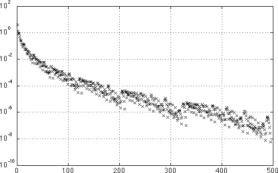
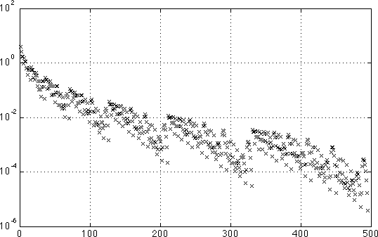
In the block sparse case, the matrices$~{}D_{\ell}$ are block diagonal, as in Figure 1(b). However, considering the underlying coefficient$~{}k$ as a random field with lognormal distribution, all of the matrices$~{}D_{\ell}$ are block dense, as in Figure 1(f). The word approximate will refer to the fact that we will approximate the (inverses of the) matrices$~{}D_{\ell}$ by (inverses of) their diagonal blocks in the action of our preconditioners. Next, a global matrix-vector multiplication in an iterative solver can be performed using formula (12), i.e., one needs to store only the constants$~{}c_{ijk}$ and the matrices $K_{i}$ for the so-called called MAT-VEC operations [10]. Here, we are interested in preconditioners that would rely only on the MAT-VEC operations as well. The top panels in Figure 1, show a decaying trend of the norms of matrices$~{}K_{i}$ with increasing index$~{}i$. This indicates, with respect to the structure of the coefficients $c_{ijk}$, that the lower order terms in the general $P^{\prime}-$th order expansion might dominate, depending on the coefficient of variation $CoV$, over the higher order terms, cf. lower panels in Figure 1. Now, the idea is to truncate, i.e., selectively drop some of the matrices$~{}K_{i}$ from the MAT-VEC operations in the action of the preconditioner. There are two possible strategies of this truncation.

First, the standard truncation is defined as follows. Let $\ell_{t}$ be maximal order of the polynomial expansion that we would like to include in the MAT-VEC operations. Then, we define the degree of truncation $M_{t}\leq M^{\prime}$ as

$$M_{t}+1=\frac{\left(N+\ell_{t}\right)!}{N!\,\ell_{t}!},$$ (17)

and the matrices $K_{i}$, for all $i=0,\dots,M_{t}$ are included in the MAT-VEC operations.

Alternatively, in the adaptive truncation we select matrices $K_{i}$ that a-priori satisfy certain criterion, e.g., such that their norm is greater than a given threshold. This is computationaly slightly more demanding because it requires finding and bookkeeping a subset of matrices$~{}K_{i}$ where $i\in\mathcal{M}_{t}\subseteq\left\{0,\dots,M^{\prime}\right\}$, however for higher values of $CoV$, or in the case of a non-monotonous decay of the matrices $K_{i}$, this might be the preferred truncation strategy.

The algorithm of the truncated block matrix-vector multiplication (tMAT-VEC) is precisely defined as follows:

Algorithm 1 (tMAT-VEC).

The truncated MAT-VEC multiplication $w=\mathcal{P}_{\ell}v$ is performed as

$$w_{\left(j\right)}=\sum_{k=0}^{M}\sum_{i\in\mathcal{M}_{t}}c_{ijk}K_{i}v_{\left(k\right)},$$ (18)

where $j,k$ are suitable subsets of $\left\{0,\dots,M\right\}$ selecting blocks of the global Galerkin matrix to be multiplied with, and the truncation is defined by a set $\mathcal{M}_{t}\subseteq\left\{0,\dots,M^{\prime}\right\}$ selecting the matrices $K_{i}$ for the MAT-VEC operation.

The notation $\mathcal{P}_{\ell}$ used in Algorithm 1 will correspond in Algorithms 2 and 3 to either $\mathcal{B}_{\ell}$, $\mathcal{C}_{\ell}$, $\mathcal{E}_{\ell}$, or $\mathcal{F}_{\ell}$, and it will denote the corresponding truncated variants of the block matrix-vector multiplications by the blocks $B_{\ell}$, $C_{\ell}$, $E_{\ell}$ or $F_{\ell}$ from (15) and (16). We note that the full MAT-VEC operation is obtained by setting $\ell_{t}=P^{\prime}$ in (17) so that $M_{t}=M^{\prime}$.

Next, let us introduce some additional notation. Considering (15), problem (14) can be rewritten as

$$\left[\begin{array}[c]{cc}A_{P-1}&B_{P}\\ C_{P}&D_{P}\end{array}\right]\left[\begin{array}[c]{c}u_{P}^{P-1}\\ u_{P}^{P}\end{array}\right]=\left[\begin{array}[c]{c}f_{P}^{P-1}\\ f_{P}^{P}\end{array}\right],$$ (19)

which motivates the following notation for a vector$~{}x_{\ell}$, where $\ell=1,\dots,P$, cf. Figure 2, as

$$x_{\ell}=\left[\begin{array}[c]{c}x_{\ell}^{\ell-1}\\ x_{\ell}^{\ell}\end{array}\right],\text{ or }x_{\ell}=\left[\begin{array}[c]{c}x_{\left(0\right)}\\ \vdots\\ x_{\left(\ell\right)}\end{array}\right]\text{.\quad So then }x_{\ell}^{\ell-1}=\left[\begin{array}[c]{c}x_{\left(0\right)}\\ \vdots\\ x_{\left(\ell-1\right)}\end{array}\right]\text{, and }x_{\ell}^{\ell}=x_{\left(\ell\right)}\text{.}$$ (20)

Note that $x_{\left(0\right)}=x_{1}^{0}=x_{0}$, and we will also for brevity denote $x_{\ell}=x_{\left(0:\ell\right)}$. We are ready to formulate now the two preconditioners. First, we recall the algorithm of the hierarchical Schur complement preconditioner (hS) from [15, Algorithm 5]. Then, we formulate the algorithm of the hierarchical Gauss-Seidel preconditioner (hGS).

Algorithm 2 (Hierarchical Schur complement preconditioner (hS)).

The preconditioner $M_{hS}:r_{P}\longmapsto v_{P}$ for system (14) is defined as follows:

for $\ell=P,\ldots 1$,

split the residual$~{}r_{\ell}$, based on the hierarchical structure of matrices, as

$$r_{\ell}=\left[\begin{array}[c]{c}r_{\ell}^{\ell-1}\\ r_{\ell}^{\ell}\end{array}\right],$$ (21)

compute the pre-correction as

$$g_{\ell-1}=r_{\ell}^{\ell-1}-\mathcal{B}_{\ell}\mathcal{D}_{\ell}^{-1}r_{\ell}^{\ell}.$$ (22)

If $\ell>1$, set

$$r_{\ell-1}=g_{\ell-1}.$$ (23)

Else (if $\ell=1)$, solve the system $A_{0}v_{0}=g_{0}$.

end

for $\ell=1,\ldots P$,

compute the post-correction, i.e., set $v_{\ell}^{\ell-1}=v_{\ell-1}$, solve

$$v_{\ell}^{\ell}=\mathcal{D}_{\ell}^{-1}\left(r_{\ell}^{\ell}-\mathcal{C}_{\ell}v_{\ell}^{\ell-1}\right),$$ (24)

and concatenate

$$v_{\ell}=\left[\begin{array}[c]{c}v_{\ell}^{\ell-1}\\ v_{\ell}^{\ell}\end{array}\right].$$ (25)

If $\ell<P,$ set $v_{\ell+1}^{\ell}=v_{\ell}$.

end

Algorithm 3 (Hierarchical Gauss-Seidel preconditioner (hGS)).

The preconditioner $M_{hGS}:r_{P}\longmapsto v_{P}$ for system (14) is defined as follows:
set the initial solution $u_{P}$ and update it in the following steps,

$$v_{\left(0\right)}=\mathcal{D}_{0}^{-1}\left(r_{\left(0\right)}-\mathcal{F}_{0}v_{\left(1:P\right)}\right),$$ (26)

for $\ell=1,\ldots P-1$,

$$v_{\left(\ell\right)}=\mathcal{D}_{\ell}^{-1}\left(r_{\left(\ell\right)}-\mathcal{E}_{\ell}v_{\left(0:\ell-1\right)}-\mathcal{F}_{\ell}v_{\left(\ell+1:P\right)}\right),$$ (27)

end

$$v_{\left(P\right)}=\mathcal{D}_{P}^{-1}\left(r_{\left(P\right)}-\mathcal{E}_{P}v_{\left(0:P-1\right)}\right),$$ (28)

for $\ell=P-1,\ldots 1$,

$$v_{\left(\ell\right)}=\mathcal{D}_{\ell}^{-1}\left(r_{\left(\ell\right)}-\mathcal{E}_{\ell}v_{\left(0:\ell-1\right)}-\mathcal{F}_{\ell}v_{\left(\ell+1:P\right)}\right),$$ (29)

end

$$v_{\left(0\right)}=\mathcal{D}_{0}^{-1}\left(r_{\left(0\right)}-\mathcal{F}_{0}v_{\left(1:P\right)}\right).$$ (30)

In our implementation, we initialize $u_{P}=0$ in Algorithm 3. Then the multiplications of$~{}\mathcal{F}_{\ell}$, $\ell=0,\dots,P-1$, by this zero vector will vanish from (26)-(27). This also reduces the computational cost of the MAT-VEC operations.

We have already mentioned that the approximate variants of the two preconditioners are obtained by replacing the solves with the blocks $\mathcal{D}_{\ell}$, $\ell=1,\dots,P$, by the corresponding diagonal block solves, cf. the right panel of Figure 3.

4.1 Computational cost considerations

In order to compare the computational cost of the preconditioners, we first recall two common solution algorithms against which comparisons will be discussed. First, let us define matrices $G_{\alpha}$, $\alpha=0,\dots,M^{\prime}$, using the coefficients $c_{ijk}$ as

$$G_{\alpha}=c_{\alpha jk},\qquad j=0,\dots,M,\quad k=0,\dots,M.$$

Let the symbol $\otimes$ denote the Kronecker product. The mean-based preconditioner [10, 11] is defined as

$$M_{mb}=\text{diag}\left(G_{0}\right)\otimes A_{0}.$$ (31)

Next, let us define a matrix

$$G=\sum_{\alpha=0}^{M^{\prime}}\frac{\text{tr}\left(A_{\alpha}^{T}A_{0}\right)}{\text{tr}\left(A_{0}^{T}A_{0}\right)}G_{\alpha}.$$

The Kronecker product preconditioner [12] is defined as

$$M_{K}=G\otimes A_{0}=\left(G\otimes I_{N_{\text{dof}}}\right)\left(I_{M+1}\otimes A_{0}\right)=\left(I_{M+1}\otimes A_{0}^{-1}\right)\left(G^{-1}\otimes I_{N_{\text{dof}}}\right).$$ (32)

The multiplication of $\left(I_{M+1}\otimes A_{0}^{-1}\right)$ by a vector is essentially the same as an application of the mean-based preconditioner, and an effficient implementation of $\left(G^{-1}\otimes I_{\text{ndof}}\right)$ is described in [22]. We can immediately see from (31) that the mean based-preconditioner requires $M+1$ solves with the matrix $A_{0}$ of size $\left(N_{\text{dof}}\times N_{\text{dof}}\right)$, and from (32) that the Kronecker product preconditioner requires in addition $N_{\text{dof}}$ solves with the matrix$~{}G$ of size $\left(\left(M+1\right)\times\left(M+1\right)\right)$, which requires $\mathcal{O}\left(N_{\text{dof}}\times\left(M+1\right)^{2}\right)$ operations if a Cholesky decomposition of $G$ is available. Both of our approximate hierarchical preconditioners require 2$\left(M+1\right)$ solves with the diagonal blocks of the global Galerkin matrix, and a certain number of matrix-vector multiplications with stiffness matrices$~{}K_{i}$. The number of these multiplications depends on the degree of truncation of the MAT-VEC operations, and it is denoted by $nz\left(c_{ijk}\right)$ in Tables 5 and 6. Clearly, the Kronecker product preconditioner is very efficient if (i) it is possible to obtain a Cholesky decomposition of$~{}G$, and (ii) the number of spatial degrees of freedom $N_{\text{dof}}$ is not too large. Moreover, it was assumed in [11, 12] that a solve with $A_{0}$ can be performed in $\mathcal{O}\left(N_{\text{dof}}\right)$ operations using a multigrid solver. However, in situations when the multigrid solver is not suitable or the size of the discretized spatial problem is too large, the question of selecting block solvers becomes much more delicate. For example, we might even consider “inner” Krylov iterations for the solves with the diagonal blocks. The preconditioner would thus become variable and we would also need to make a careful choice of the Krylov iterative method used for the global (“outer”) iterations. Our initial experiments with such choice were successful, and the present work is the first step in the development of such solvers.

5 Numerical experiments

We have implemented the stochastic Galerkin finite element method for the model problem (1)-(2) on a two-dimensional domain with dimensions $[0,1]\times[0,1]$ uniformly discretized by $10\times 10$ Lagrangean finite elements. The mean value of the coefficient$~{}k$ was set to$~{}k_{0}=1$, the correlation length $L=0.5$, and we have used the covariance kernel in (6) as

$$C_{g}\left(x,y\right)=\sigma^{2}\exp\left(-\frac{\left\|x-y\right\|_{1}}{L}\right),$$ (33)

where $\sigma$ denotes the standard deviation. In the experiments reported in Tables 1, 2 and 4 we have set $\sigma=1$, and so the coefficient of variation $CoV=\sigma/k_{0}=100\%$. We have compared convergence of the flexible conjugate gradients, the mean-based preconditioner (mb), the Kronecker product preconditioner (K), the hierarchical Schur complement preconditioner (hS), the approximate hierarchical Schur complement preconditioner (ahS), symmetric (block) Gauss-Seidel preconditioner (GS), and the approximate hierarchical Gauss-Seidel preconditioner (ahGS). We note that in all cases we have observed essentially the same convergence of the standard and flexible conjugate gradients [19]. We have also tested direct and iterative solvers, with the same tolerance as for the outer iterations, for the inner block solves. Our experiments indicate that the convergence in terms of outer (global) iteration counts is not sensitive to the particular choice of inner block solves. The results are summarized in Tables 1-6. First, we have compared the convergence using the preconditioners with no truncation, varying either of the stochastic dimension$~{}N$, the order of polynomial expansion $P$, the coefficient of variation $CoV$ or the mesh size $h$, and keeping other parameters fixed. These results are, respectively, reported in Tables 1-4. Looking at the tables, we see that the hS preconditioner performs best, followed by the GS preconditioner. On the other hand, the convergence of the ahS preconditioner quickly deteriorates, whereas the convergence of the aGS is quite similar to the GS. In fact, it is quite interesting to note from Table 3 that the convergence of the ahS begins to deteriorate for values of $CoV>25\%$, however the aGS remains comparable to the GS preconditioner for values of $CoV$ at around$\ 100\%$. From Table 4 we see that the dependence on the mesh size$~{}h$ is not very significant. Tables 5 and 6 contain results obtained for variable coefficients of variation $CoV=\sigma_{\log}/\mu_{\log}$ and different truncation strategy of the MAT-VEC operations in the action of the preconditioners, which is guided by the decay of the norms of the stiffness matrices$~{}K_{i}$ obtained from the finite element discretization of the generalized polynomial chaos expansion of the random coefficient$~{}k\left(x,\omega\right)$, cf. Figure 1. Table 5 contains results obtained using the standard truncation. First, we note that setting $\ell_{t}=0$ yields to use of only the matrix$~{}K_{0}$ in the action of the ahS, GS, and ahGS preconditioners. So the resulting preconditioners are in this case block diagonal and because they are symmetric, their application is the same as using twice the mean-based preconditioner. On the contrary, the performance of the hS preconditioner might be slightly better even with $\ell_{t}=0$, in particular for higher values of $CoV$, but this is because the hS preconditioner performs solves with the full submatrices$~{}D_{\ell}$. However, we can see that this does not correspondingly improve the convergence, and use of the off-diagonal blocks seems to be warranted. Indeed, the convergence improves with more included into the MAT-VEC operations in the action of all of the preconditioners. In particular, we see that for values of $CoV$ at around $25\%$ it is sufficient to include only the five matrices corresponding to the linear terms of the coefficient expansion. On the other hand, even for higher values of $CoV$ there seems to be no reason for the GS and aGS preconditioners to use the matrices obtained from the polynomials of higher order than the expansion of the solution, i.e., the computational cost of these preconditioners can be reduced more than twice. Finally, Table 6 contains results obtained with the adaptive truncation, where the tolerance$~{}\tau$ has been set such that the matrices $K_{i}$ for which $\text{max}_{jk}\left(c_{ijk}\right)\times\mathrm{norm}(K_{i})<\tau$ are dropped from the MAT-VEC operations in the action of the preconditioners. As before, only few matrices need to be used in order to significantly improve the convergence. Moreover, it appears that setting the threshold$~{}\tau$ too low might have a negative impact on the convergence of the ahS and ahGS preconditioners. In particular, rather surprisingly, even with higher values of $\tau$ the convergence of the truncated ahGS is comparable to the convergence of GS with no truncation (setting $\tau=0$). We can in fact see that, e.g., for the values of $CoV$ equal to$\ 100\%$ and $150\%$, with value $\tau=10$, the convergence of the ahGS is essentially the same as the convergence of the GS preconditioner with no truncation.

Table 1: Convergence of flexible conjugate gradients for the global matrix $A$ obtained by the gPC expansion of the lognormal field with $CoV=\sigma_{\log}/\mu_{\log}=100\%$, and $\mu_{\log}=1$, preconditioned by the mean-based preconditioner (mb), Kronecker product preconditioner (K), hierarchical Schur complement (hS), approximate hierarchical Schur complement (ahS), block Gauss-Seidel (GS) and approximate hierarchical block Gauss-Seidel (ahGS) preconditioners. Polynomial degree is fixed to $P=4$, and the stochastic dimension $N$ is variable. Here, $ndof$ is the dimension of $A$, $iter$ is the number of iterations with the relative residual tolerance $10^{-8}$, and $\kappa$ is the condition number estimate from the Lánczos sequence in conjugate gradients.

setup		mb		K		hS		ahS		GS		ahGS
$N$	$ndof$	$it$	$\kappa$	$it$	$\kappa$	$it$	$\kappa$	$it$	$\kappa$	$it$	$\kappa$	$it$	$\kappa$
1	605	48	28.76	18	3.87	15	3.40	15	3.40	15	3.42	15	3.42
2	1815	61	37.16	32	10.10	16	3.62	27	8.06	17	3.75	16	3.45
3	4235	62	38.07	32	10.30	16	3.76	31	10.77	17	3.74	18	4.35
4	8470	66	43.65	37	13.60	16	4.17	38	15.28	19	4.29	19	4.74

Table 2: Convergence of flexible conjugate gradients for the global matrix $A$ preconditioned by the mean-based preconditioner (mb), Kronecker product preconditioner (K), hierarchical Schur complement (hS), approximate hierarchical Schur complement (ahS), block Gauss-Seidel (GS) and approximate hierarchical block Gauss-Seidel (ahGS) preconditioners. stochastic dimension is fixed to $N=4$, and the polynomial degree $P$ is variable. The other headings are same as in Table 1.

setup		mb		K		hS		ahS		GS		ahGS
$P$	$ndof$	$it$	$\kappa$	$it$	$\kappa$	$it$	$\kappa$	$it$	$\kappa$	$it$	$\kappa$	$it$	$\kappa$
1	605	15	3.50	14	2.44	7	1.39	11	1.76	8	1.39	8	1.31
2	18	28	8.95	21	4.74	10	1.93	16	3.04	12	1.97	11	1.76
3	4235	44	20.04	29	8.28	13	2.80	24	6.09	15	2.87	14	2.58
4	8470	66	43.65	37	13.60	16	4.17	38	15.28	19	4.29	19	4.74

Table 3: Convergence of flexible conjugate gradients for the global matrix $A$ preconditioned by the mean-based preconditioner (mb), Kronecker product preconditioner (K), hierarchical Schur complement (hS), approximate hierarchical Schur complement (ahS), block Gauss-Seidel (GS) and approximate hierarchical block Gauss-Seidel (ahGS) preconditioners. Stochastic dimension and polynomial degree are fixed to $N=P=4$, and the coefficient of variation $CoV$ is variable $\mu_{\log}=1$. The other headings are same as in Table 1.

setup	mb		K		hS		ahS		GS		ahGS
$CoV\,(\%)$	$it$	$\kappa$	$it$	$\kappa$	$it$	$\kappa$	$it$	$\kappa$	$it$	$\kappa$	$it$	$\kappa$
25	16	3.24	14	2.37	7	1.18	8	1.25	7	1.18	6	1.12
50	29	9.36	22	4.96	10	1.78	14	2.45	11	1.77	10	1.62
75	46	22.21	30	8.73	13	2.85	23	6.01	15	2.82	14	2.69
100	66	43.65	37	13.60	16	4.17	38	15.28	19	4.29	19	4.74
125	85	72.76	45	19.79	19	5.54	58	36.34	23	5.98	26	8.21
150	103	107.07	52	27.02	21	6.85	84	77.73	26	7.75	35	13.74

Table 4: Convergence of flexible conjugate gradients for the global matrix $A$ preconditioned by the mean-based preconditioner (mb), Kronecker product preconditioner (K), hierarchical Schur complement (hS), approximate hierarchical Schur complement (ahS), block Gauss-Seidel (GS) and approximate hierarchical block Gauss-Seidel (ahGS) preconditioners. Stochastic dimension and polynomial degree are fixed to $N=P=4$, the coefficient of variation is $CoV=100\%$, and the mesh size $h$ is variable. The other headings are same as in Table 1.

setup		mb		K		hS		ahS		GS		ahGS
$h$	$ndof$	$it$	$\kappa$	$it$	$\kappa$	$it$	$\kappa$	$it$	$\kappa$	$it$	$\kappa$	$it$	$\kappa$
$1/5$	2520	59	40.62	35	14.06	15	3.84	35	15.43	18	3.99	19	4.91
$1/10$	8470	66	43.65	37	13.60	16	4.17	38	15.28	19	4.29	19	4.74
$1/15$	17920	68	44.42	39	13.87	16	4.24	39	15.81	19	4.38	20	4.72
$1/20$	30870	69	44.89	39	14.07	17	4.25	40	16.23	19	4.37	20	4.78
$1/25$	47320	69	44.94	40	14.13	17	4.26	41	16.38	20	4.40	20	4.81
$1/30$	67270	71	45.11	40	14.04	17	4.26	41	16.38	19	4.37	20	4.75

Table 5: Convergence of the flexible conjugate gradients for the global stochastic Galerkin matrix preconditioned by the mean-based preconditioner (mb), Kronecker product preconditioner (K),  hierarchical Schur complement (hS), approximate hierarchical Schur complement (ahS), block Gauss-Seidel (GS) and approximate hierarchical block Gauss-Seidel (ahGS) preconditioners with a variable degree of truncation of the MAT-VEC operations in the action of the preconditioner. Here $\ell_{t}$ is the maximum polynomial order of the coefficient expansion used in the construction of the preconditioner, so that $M_{t}+1$ is the degree of truncation of the MAT-VEC operations i.e., the number of retained matrices, $nz(c_{ijk})$ is the number of nonzeros in the truncated tensor $c_{ijk}$, $iter$ is the number of iterations with the relative residual tolerance $10^{-8}$, and $\kappa$ is the condition number estimate from the Lánczos sequence in flexible conjugate gradients.

setup			hS		ahS		GS		ahGS
$\ell_{t}$	$M_{t}+1$	$nz(c_{ijk})$	$it$	$\kappa$	$it$	$\kappa$	$it$	$\kappa$	$it$	$\kappa$
$CoV=25\%$  ( mb:   $it=16$  $\kappa=3.24$,    K:   $it=14$  $\kappa=2.37$ )
0	1	70	16	3.20	16	3.19	16	3.19	16	3.19
1	5	350	8	1.27	8	1.33	7	1.23	7	1.23
2	15	1210	7	1.21	8	1.25	7	1.20	6	1.17
3	35	2610	7	1.18	8	1.25	7	1.17	6	1.11
4	70	4980	7	1.18	8	1.25	7	1.18	6	1.12
8	495	12585	7	1.18	8	1.25	7	1.18	6	1.12
$CoV=50\%$  ( mb:   $it=29$  $\kappa=9.36$,    K: $it=22$  $\kappa=4.96$)
0	1	70	28	8.90	28	8.99	28	8.99	28	8.99
1	5	350	14	2.54	15	2.83	14	2.54	14	2.54
2	15	1210	13	2.47	14	2.74	12	2.15	11	2.12
3	35	2610	10	1.79	14	2.44	10	1.68	10	1.69
4	70	4980	10	1.79	13	2.39	11	1.78	10	1.68
8	495	12585	10	1.78	14	2.45	11	1.77	10	1.62
$CoV=100\%$  ( mb:   $it=66$  $\kappa=43.65$,    K: $it=37$  $\kappa=13.60$)
0	1	70	53	32.88	58	39.94	58	39.94	58	39.94
1	5	350	32	11.83	35	14.29	33	12.88	33	12.88
2	15	1210	32	12.31	35	15.13	28	9.35	29	10.05
3	35	2610	20	5.03	36	14.32	19	4.64	22	6.23
4	70	4980	20	5.24	32	11.92	19	4.55	20	5.33
8	495	12585	16	4.17	38	15.28	19	4.29	19	4.74
$CoV=150\%$  ( mb:   $it=103$  $\kappa=107.067$,    K: $it=52$  $\kappa=27.0203$)
0	1	70	71	61.44	89	90.18	89	90.18	89	90.18
1	5	350	51	29.92	59	39.66	57	36.85	57	36.85
2	15	1210	51	30.18	60	42.06	46	24.26	50	27.53
3	35	2610	31	11.06	71	55.98	30	10.17	40	19.53
4	70	4980	32	12.05	58	38.08	28	9.42	34	13.86
8	495	12585	21	6.85	84	77.73	26	7.75	35	13.74

Table 6: Convergence of the flexible conjugate gradients for the global stochastic Galerkin matrix preconditioned by the mean-based preconditioner (mb), Kronecker product preconditioner (K), hierarchical Schur complement (hS), approximate hierarchical Schur complement (ahS), block Gauss-Seidel (GS) and approximate hierarchical block Gauss-Seidel (ahGS) preconditioners with a variable degree of truncation of the MAT-VEC operations in the action of the preconditioner. Here $\tau$ is the tolerance such that the matrices $K_{i}$ for which $\text{max}_{jk}\left(c_{ijk}\right)\times\mathrm{norm}(K_{i})<\tau$ are dropped from the MAT-VEC operations in the action of the preconditioner and $N_{\text{adapt}}$ is the number of retained matrices, $nz(c_{ijk})$ is the number of nonzeros in the truncated tensor $c_{ijk}$, $iter$ is the number of iterations with the relative residual tolerance $10^{-8}$, and $\kappa$ is the condition number estimate from the Lánczos sequence in flexible conjugate gradients.

setup			hS		ahS		GS		ahGS
$\tau$	$N_{\text{adapt}}$	$nz(c_{ijk})$	$it$	$\kappa$	$it$	$\kappa$	$it$	$\kappa$	$it$	$\kappa$
$CoV=25\%$   mb:   $it=16$   $\kappa=3.24$  K:   $it=14$   $\kappa=2.37$
$10$	5	345	10	1.63	10	1.58	10	1.57	10	1.57
$1$	13	877	7	1.20	8	1.24	7	1.18	6	1.12
$0.1$	32	2057	7	1.18	8	1.24	7	1.17	6	1.12
$0$	495	12585	7	1.18	8	1.25	7	1.18	6	1.12
$CoV=50\%$   mb:   $it=29$  $\kappa=9.36$  K:   $it=22$   $\kappa=4.96$
$10$	11	677	12	2.18	13	2.24	11	1.83	11	1.83
$1$	32	1958	11	1.91	13	2.25	11	1.77	10	1.62
$0.1$	86	4765	10	1.78	14	2.41	11	1.77	10	1.62
$0$	495	12585	10	1.78	14	2.45	11	1.77	10	1.62
$CoV=100\%$   mb:   $it=66$  $\kappa=43.65$  K:   $it=37$   $\kappa=13.60$
$100$	2	92	54	34.95	63	47.94	65	51.28	65	51.28
$10$	25	1241	27	9.12	25	7.14	23	6.98	19	4.56
$1$	97	4731	18	4.48	33	12.29	19	4.55	18	4.10
$0.1$	219	8202	17	4.18	37	14.90	19	4.31	19	4.66
$0$	495	12585	16	4.17	38	15.28	19	4.29	19	4.74
$CoV=150\%$   mb:   $it=103$   $\kappa=107.07$  K:   $it=52$   $\kappa=27.02$
$100$	10	336	66	50.22	68	48.84	70	50.68	70	50.68
$10$	55	2450	30	10.89	44	20.38	29	9.49	25	6.95
$1$	171	6338	23	7.00	73	59.57	27	7.98	32	11.48
$0.1$	313	9714	22	6.86	83	76.38	26	7.74	35	13.54
$0.01$	436	11741	21	6.84	84	77.69	26	7.75	35	13.72
$0$	495	12585	21	6.85	84	77.73	26	7.75	35	13.74

6 Conclusion

We have proposed two novel strategies for constructing preconditioners for the iterative solution of the systems of linear algebraic obtained from the stochastic Galerkin finite element discretizations. Our main focus was on a class of problems with coefficients characterized by arbitrary distributions that generally yield fully block dense structure of global stochastic Galerkin matrices. The preconditioners take an advantage of the hierarchical structure of these matrices. We have, in particular, examined variants of the hierarchical Schur complement preconditioner proposed recently by the authors [15], and variants of the hierarchical block symmetric Gauss-Seidel preconditioner.

The first variant, called an approximate, replaces solves with submatrices by the associated diagonal block solves. This variant thus combines global Gauss-Seidel method with “local” block-diagonal preconditioner, which allows decoupling of blocks, and introduces a possibility for a parallelisation in an implementation. Numerical experiments with our model problem indicate that whereas the performance of the approximate version of the hierarchical Schur complement preconditioner deteriorates with the increasing values of the coefficient of variation, the convergence of the approximate hierarchical Gauss-Seidel preconditioner is quite comparable to the (non-hierarchical) block Gauss-Seidel preconditioner for the values of the coefficient of variation equal up to $100\%.$

The second variant, called truncated, is based on a truncation of the sequence of block matrix-vector multiplications, called MAT-VEC operations, used in the action of the preconditioners. The truncation can be performed using either a standard or adaptive strategy, based on the monotonicity in the decay of the stiffness matrices, and further alleviates the computational cost of the preconditioners. Our numerical experiments indicate that truncation, in particular with adaptive strategy, might not be necessarily traded off for slower convergence rates.

We have therefore proposed two strategies that are combined for optimal performance. One strategy introduces decoupled diagonal block solves, and the other reduces the overall computational cost associated with the action of a preconditioner. Considering that a multiplication of a vector by the global stochastic Galerkin matrix in each iteration of a Krylov subspace method is, of course, performed by the full MAT-VEC multiplication with no truncation, in particular the truncated version of the approximate hierarchical Gauss-Seidel preconditioner preconditioners thus offers an appealing combination of good convergence rates and a reasonable computational cost.