Searching for pulsars using image pattern recognition
Abstract
In the modern era of big data, many fields of astronomy are generating huge volumes, the analysis of which can sometimes be the limiting factor in research. Fortunately, powerful data-mining techniques have been developed by computer scientists, ready to be applied to various fields. In this paper, we present a novel artificial intelligence (AI) program that identifies pulsars from recent surveys using image pattern recognition with deep neural nets—the PICS (Pulsar Image-based Classification System) AI. The AI mimics human experts and distinguishes pulsars from noise and interference by looking for patterns from candidate plots. Different from other pulsar selection programs which searched for expected patterns, the PICS AI is taught the salient features of different pulsars from a set of human-labeled candidates through machine learning. The training candidates are collected from the Pulsar Arecibo L-band Feed Array Survey. The information from each pulsar candidate is synthesized in four diagnostic plots, which consist of image data with up to thousands of pixels. The AI takes these data from each candidate as its input and uses thousands of such candidates to train its 9000 neurons. The deep neural networks in this AI system grant it superior ability in recognizing various types of pulsars as well as their harmonic signals. The trained AI’s performance has been validated with a large set of candidates from a different pulsar survey, the Green Bank North Celestial Cap survey. In this completely independent test, PICS ranked 264 out of 277 pulsar-related candidates, including all 56 previously known pulsars and 208 of their harmonics, in the top 961 (1%) of 90008 test candidates, missing only 13 harmonics. The first non-pulsar candidate appears at rank 187, following 45 pulsars and 141 harmonics. In other words, 100% of the pulsars were ranked in the top 1% of all candidates, while 80% were ranked higher than any noise or interference. The performance of this system can be improved over time as more training data are accumulated. This AI system has been integrated into the PALFA survey pipeline and has discovered six new pulsars to date.
1 Introduction
Recent pulsar surveys such as the Pulsar Arecibo L-band Feed Array (PALFA; Cordes et al. 2006; Kaspi 2012; Lazarus 2013) survey and the Green Bank North Celestial Cap (GBNCC; Lynch et al. 2013, K. Stovall et al. in prep.) survey are expected to find—or are already finding—hundreds of new pulsars among many millions of pulsar candidates. However, the surveys are polluted by radio frequency interference (RFI) that makes it hard to pick out the pulsars from the candidates produced using simple metrics such as the signal-to-noise ratio (SNR). Human experts can look at diagnostic plots of the candidates and identify the pulsars more successfully, but it is impractical to inspect millions of candidates that way. In this paper, we present an artificial intelligence (AI) system that emulates human experts and classifies pulsar candidates using patterns from four standard diagnostic plots—the pulse profile, time-versus-phase plot, frequency-versus-phase plot, and dispersion-measure (DM) curve (see Section 2.1 for details). This system was trained with PALFA candidates classified by human experts, its parameters were tuned using a cross-validation set of candidates, and its final performance was compared against a large set of manually identified candidates from the GBNCC survey (project code: GBT09C-057). Both the PALFA and GBNCC candidates are generated using a pipeline that runs the PRESTO111http://www.cv.nrao.edu/sransom/presto/ search software (Ransom 2001; Ransom et al. 2002), but other pulsar-searching pipelines, such as the one in the Einstein@Home project (Allen et al. 2013; Knispel et al. 2013), can produce these same diagnostic plots, so it is possible to apply our AI system to most pulsar surveys with little modification.
In the past, several successful candidate-sifting schemes have been developed for different surveys. Some involve graphical interfaces which allow for the interactive selection of pulsar candidates based on the pulse period and SNR (Faulkner et al. 2004). Some apply heuristic scoring algorithms to the candidate diagnostic plots, using statistical tests, curve fitting, and a graphical interface to visually inspect the distribution of pulsar scores in the scores’ parameter space (Keith et al. 2009). An effective sorting scheme was constructed (Lee 2009; Lee et al. 2013) using a combination of six carefully designed heuristic scores. One particular score compares the candidate’s pulse frequency against the frequency distribution drawn from a large sample of the survey candidates; recognizing that the majority of candidates are RFI, this single histogram removes a large fraction of the repeatedly observed RFI, especially harmonics of the 60 Hz interference from the power supply. Eatough et al. (2010) improved the method of Keith et al. (2009) by applying machine learning (ML) to the heuristic scores. Instead of inspecting the score distribution by eye, they fed the scores into an artificial neural network and trained the network to classify candidates. Bates et al. (2012) expanded the number of scores used by fitting the candidate’s features with different model curves, and also used a neural network to combine these scores. Another comprehensive score-based system (Kaspi 2012; Lazarus 2013) was developed and has been used to find many pulsars for the PALFA survey. Most recently, Knispel et al. (2013) designed algorithms that check for outstanding signals in some of the diagnostic plots by binning the plots with pre-designed patterns in the shape of vertical lines or area patches, and applied them in the Einstein@Home project.
Notably, these previous candidate-sifting systems use heuristically-designed functions which characterize patterns in the diagnostic plots into a set of scores. Such score-based systems have some advantages. They make good use of the candidate’s properties like period, DM and computed information like the significance of the periodicity and the width/height of the summed profile. However, such systems often rely on matching candidates with some pre-designed patterns, such as a Gaussian-like peak. Some of these designed patterns do not match pulsars with multiple pulse peaks well. When these designed patterns do match the candidate, they tend to average out the details and small features in the diagnostic plot. These small features can sometimes be very useful in distinguishing pulsars from RFI. Some score-based systems select pulsar candidates by drawing the score distributions from known pulsars. Such systems may be biased against rare types of pulsars, such as pulsars with wider profiles, skewed DM curves or low signal strength.
In contrast, the PICS AI applies image pattern recognition directly to the original diagnostic plots, and determines what patterns to match through machine learning. Using the original diagnostic plots allows the AI to utilize the detailed information in the plots. Using ML allows us to train the AI with a wide variety of pulsar candidates. A significant fraction of our training candidates are pulsars or their harmonics with weak, broad, or multi-peak pulse profiles (for example, a harmonic signal at period of the fundamental would be a factor of broader and weaker and a harmonic at period would have two peaks). As a result, the PICS AI is sensitive not only to pulsar candidates but also to their harmonics. In fact, one of the new pulsars discovered by PICS, PSR J1914+08 (Figure 2), was identified from its , and harmonics. In this case, the fundamental frequency was missed by the PALFA pipeline due to RFI. Finally, an important feature of the PICS AI is that it neglects information such as the candidate’s period, DM and sigma value. Instead, it focuses on only the details in the normalized diagnostic plots. This feature makes it a good complement to the score-based systems.
This paper introduces a new approach to the candidate-sifting problem using supervised ML based on image patterns. In Section 2, we describe the candidate plots which contain the physical features distinguishing them as pulsars, and we detail the data-preparation process required to adapt these plots as inputs to the ML system. We also describe the structure of the PICS AI system. In Section 3, we detail the AI’s test performance and results from classifying GBNCC data. Finally in Section 4, we discuss the results and the AI system’s unique strengths and features.
2 Implementation
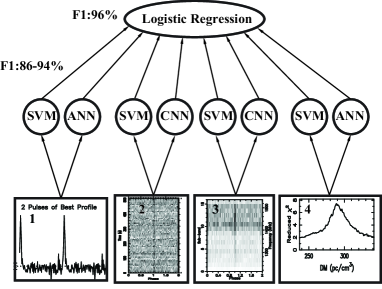
The diagnostic plot that a human expert relies on to identify a pulsar contains several important subplots. In order to combine the information from these subplots, we constructed the PICS AI with a two-layer hierarchy (Figure 1). The first layer consists of a group of ML classifiers trained to look at different subplots, providing a pool of experts capable of recognizing pulsar patterns; while the second layer combines the classifications from first layer to classify the candidate. Each first-layer classifier rates how “pulsar-like” a particular subplot of the candidate is with a number between 0 (not a pulsar) and 1 (a pulsar), giving a prediction matrix that is the output of the first layer. These votes are fed into a second-layer classifier which learns to properly weight these votes and forms a final consensus on how pulsar-like a candidate is.
In this section we provide a detailed discussion of the PICS AI implementation222The AI source code and a trained classifier are accessible on githubhttps://github.com/zhuww/ubc_AI, starting from the most important subplots that the AI uses.
2.1 Four features
Our goal is to train an AI program that mimics human experts. Here we first introduce how the PALFA pipeline finds pulsar candidates and then discuss which features human experts look for when identifying promising candidates.
The PALFA survey uses the 7-beam L-band (1.4 GHz) receiver at the Arecibo observatory. The survey takes 5-minute snapshots of the Galactic plane. In recent observations, data were taken using the Mock spectrometer, which has a 65.5 s sampling time and 960 frequency channels covering 322.6 MHz of bandwidth. The data from each beam are analyzed using a PRESTO-based pulsar-searching pipeline.
Pulsar radio emission is a broadband signal originating from kpc distances. Therefore, the signal is dispersed by the ionized interstellar medium. This causes the low-frequency components of a signal to arrive later than the ones at higher frequency. The delay between the two frequencies and is proportional to DM where DM, the dispersion measure, is the column density of free electrons along the line of sight. This is non-zero and remains nearly constant for a pulsar. Because of this, the wide-band signals of pulsars need to be recorded into narrow frequency channels to prevent smearing by dispersion. PRESTO first searches for narrow band or non-dispersed periodic signals in the raw channelized data and removes them, since they are likely terrestrial. Then it generates time series for an array of DM values by adding appropriate time delays to each frequency channel. The range of DM searched is DM, which easily encompasses the expected Galactic interstellar dispersion for all lines of sight in the PALFA survey (Cordes & Lazio 2001) and also maintains sensitivity to any possible highly-dispersed extragalactic radio sources (e.g. Lorimer et al. 2007; Thornton et al. 2013, L. Spitler et al. in prep.). After that it searches for periodic signals in the “de-dispersed” time series using a Fourier Transform and harmonic summing, and picks out the significant periodicity peaks in the power spectrum (see Ransom 2001 for details). For each candidate periodicity, PRESTO folds the de-dispersed time series into a 3D data cube (time interval, phase and channel frequency) using the period, and stores the folded data in a pfd format file together with data descriptors such as the date and coordinates of the observation. These pfd files can later be converted to candidate diagnostic plots using routines in the PRESTO software suite.
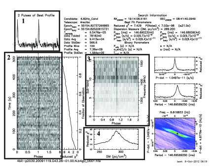
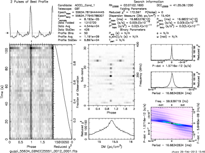
Direct inspection of the folded 3D data array is inconvenient, so it is usually projected into several lower-dimensional plots. The PRESTO routine show_pfd is designed to display the pfd file as a candidate plot that contains several of these projections. Figure 2 is an example pulsar candidate plot, with the most important subplots highlighted.
1. Summed profile: One can sum all frequency channels and time intervals to create a summed intensity-versus-phase pulse profile. Pulse profiles of real pulsars are usually composed of one or several very narrow peaks, though there are some known pulsars with pulse profiles which are broad and/or contain multiple peaks.
2. Time-versus-phase plot: This plot is obtained by summing the data over the different frequency channels, leaving the pulse profile as averaged over subintervals of the observation. One or more vertical stripes in this plot indicates that a pulsed signal was observed for the duration of the scan.
3. Frequency-versus-phase plot: Summing the data cube over the different time intervals leaves the frequency-versus-phase plot. The presence of one or more persistent vertical lines in this subplot, as in the example, indicates a broadband signal during the pulsed emission, as expected for a pulsar candidate. However, scintillation caused by the interstellar medium may affect a pulsar’s signal, degrading the signal in some frequency channels.
4. DM curve: The plotting program searches over a range of DMs around the best reported value. For each DM trial, it de-disperses the data cube accordingly and calculates the of the de-dispersed pulse profile against a horizontal line fit. The DM curve is a plot of the trial DMs against their corresponding values. A large value indicates that the periodic signal deviates strongly from simple white noise. The DM curve of a real pulsar will likely peak at a non-zero value unless affected by strong RFI.
These are the four most important features that human experts look at when classifying candidates, and they are the inputs to our AI system.
2.2 Data preparation
The application of pattern recognition to pulsar candidates is not a trivial task. This is because the integration time of survey observations may vary, and the number of phase bins with which the data are folded also changes depending on the period of the candidate. As a result, the number of data points in the subplots can vary from candidate to candidate. For ML to work, we need to carefully prepare these data, and make sure the input data blocks for a particular classifier have identical shape and size.
We extract the key feature plots from the pfd files. These plots consist of 1D data arrays (summed profile or DM curve) and 2D data (time/frequency-versus-phase plot). The sizes of the data arrays vary from candidate to candidate. For example, some candidates have 64 phase bins, while others may have only 32 bins; some candidates have 50 time steps, while others have 100. This is a result of the search pipeline, which uses fewer phase bins and more time steps for short period pulsars, and more phase bins with fewer time steps for long period pulsars—in either case, the number of pulses coherently added in each time interval is roughly the same. For ML to work on these plots, the features should have the same size and scale, so we down-sample or interpolate the data to a uniform size: 64 bins for the summed profile, 6464 (or 4848 depending on the classification algorithm, see Table 1 for details) bins for the time/frequency-versus-phase plot, and 60 bins for the DM curve. Piecewise linear interpolation was used for the 1D data and spline interpolation333The 2D interpolation routine in scipy.ndimage.interpolation.map_coordinates was used. for the 2D data. We also normalize the data to zero median and unit variance to remove the absolute scale of the plots. For the 2D image arrays, normalization is performed line-by-line along the phase axis, which removes instrumental variations over the course of the observation and across the observing band, but maintains the variance in signal across the phase—this should be dominated by the pulsar signal.
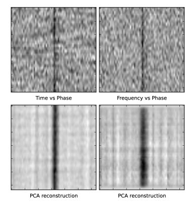
Once the plots are resized and normalized, we can use them to train a ML system. However, the thousands of pixels in the 2D plots may slow down the training process for the support vector machine (Section 2.3) classifiers. In this cases the number of internal parameters requiring training is proportional to the size of the input data, so to speed up the computation, the image features (time/frequency versus phase plot) are characterized by a principal component analysis444http://scikit-learn.org/stable/modules/generated/sklearn.decomposition.PCA.html (PCA). The PCA algorithm uses a singular value decomposition to compute a limited set of basis images from the training data. An unknown candidate’s data, then, has a new representation as the set of eigenvalues resulting from the projection onto these basis images. In this way, we can compress the image features from thousands of numbers per candidate to only 24 numbers555The number of singular vectors used in the decomposition is a free parameter in the AI system, but is fixed by optimizing the performance in cross-validation tests., greatly reducing the number of parameters required in a fit. Figure 3 shows the original 2D images of a pulsar candidate and their reconstructions from the most significant 24 PCA components. One can see that the PCA reconstructions capture the important features in the images, especially the vertical stripes. By filtering out the weaker PCA components we also reduce the noise level in the reconstructed image. Some image classifiers trained much faster with PCA-compressed features and perform as well as those trained with full-sized images. However, we did not apply the PCA-compression for the deep-neural-net classifiers because they perform significantly better without it.
One last challenge was to prevent the AI from developing any phase-related bias. In principle, a candidate’s pulse may appear at any phase, but in practice many candidates peak at phase 0 or 0.5. We found that an earlier version of the AI failed to detect some good candidates that peaked away from phase 0 or phase 0.5. We resolved this problem by shifting candidates’ strongest peaks to phase 0.5 before feeding them to the AI. The resulting AI was tested with candidates of random phase and showed no sign of bias.
In summary, the data-preparation procedure for all candidates fed into the AI system involves rescaling the data to zero median and unit variance, shifting the peak intensity to a phase of 0.5, down-sampling or interpolating onto a standardized grid and, optionally, applying PCA.
2.3 Two-Layer AI: a committee of experts
The first layer of PICS (see Figure 1) uses a combination of two ML algorithms on each of the four subplots, giving eight ratings in total. The set of ML algorithms includes artificial neural networks (ANN; see Section 2.4 for detail), convolutional neural networks (CNN666https://github.com/aberndsen/NeuralNetwork; see Section 2.5 for detail) and support vector machine (SVM777http://scikit-learn.org/stable/modules/svm.html; an algorithm that finds a direction in the parameter space on which the distance between the two classes of data points are maximized; see Chang & Lin (2011) and Pedregosa et al. (2011) for the implementation details). The choice of which algorithms to use was determined both by their individual performance and their benefit to the overall performance. It should be noted that the combinations were the result of extensive testing, including using other standard ML algorithms such as decision trees. In the end, PICS uses an ANN with one hidden layer of logistic units and a radial kernel SVM classifier on each of the 1D subplots (pulse profile, DM curve), and it uses a CNN and SVM on each of the 2D subplots (pulse interval versus phase, pulse frequency versus phase).
In the second layer, we combine the scores from the eight first-layer classifiers using another ML classifier (Figure 1). Several algorithms are appropriate for this purpose, and we tested logistic regression (LR), ANN and SVM algorithms. The best performance was from a simple LR with L2 penalty888A L2 penalty means the algorithm also tries to minimize , preventing the weights from growing too large. is a small control parameter., and this option was chosen for the second layer of the PICS system. The LR algorithm assigns each of the first-layer scores () a weight (), computes their weighted sum, and converts this sum to a probability using the logistic function
| (1) |
The LR algorithm finds the best set of that minimize the classification errors in the training data.
In order to test how well the classifier can perform on new data, we employ a validation test. To do this, we first split the labelled PALFA data into a training set and a test, or cross-validation, set. We use the training data to train the classifiers and the validation data to test them. Because the validation data were set aside from the beginning, this test result is a reliable estimate of the classifier’s performance.
A commonly used performance metric is the score, defined as the harmonic average of precision (the ratio of true pulsars to the total number of candidates ranked as a pulsar) and completeness (the ratio of ranked true pulsars to the total number of pulsars in the validation set)
| (2) |
The score from validation tests may vary slightly from test to test due to random fluctuations. We run many iterations of training and testing in order to find a reliable estimate of it. Every iteration starts with randomly splitting the labeled data into new groups of training and test data, so the new test will be different from the previous one (See Table 1).
The classifiers in both layers of the system all have internal design parameters that need to be fixed. This is accomplished by a grid search over the possible values of the design parameters, and is fixed by the set that maximize the score in a validation test. The optimized parameters of the eight classifiers and their test performance on each feature plot is listed in Table 1. The performance is also depicted in Figure 1, which shows the overall structure of the PICS system.
Finally, in this particular searching-for-pulsars problem, it might seem that we should prefer a classifier with higher completeness than precision. In general, maximizing the precision alone would result in a cautious AI system which would miss a lot of true pulsars, while maximizing completeness would bring in a lot of false positives. When training the PICS, we preferred a balanced AI that maximizes . This is because we want to improve the AI’s completeness when we add more varieties of pulsars to the training data and we also want to improve its precision when we add more RFI candidates, to emphasize on one metric will hinder our ability to improve the other. When applying the AI in practice, we can adjust its completeness and precision to our needs by changing the cut on , the AI probability score.
2.4 The neural networks
In the first layer of PICS, we used the ANN for the 1D subplots and the CNN for the 2D subplots, they are different types of neural network. In this Section, we briefly introduce some terminology common to the understanding of both these neural networks. For the detail implementation of LR and SVM please refer to Pedregosa et al. (2011) and Chang & Lin (2011).
Biologically, a neural network is a collection of neurons connected by synapses, where individual neurons respond, or “fire”, to different inputs. An artificial neural network is the computer analog, modelled as a function of many inputs (synapses) to produce a single output. These functions are often called activation functions , and typically have finite range for classification purposes. The most commonly used activation functions are the logistic (sigmoid) function and the hyperbolic tangent function . The former maps any float input to a number between 0 and 1, the latter maps to a number between 1 and 1.
In the ANN, these neurons are distributed among different layers. All neurons in a single layer receive the same inputs from the previous layer , but weights the signals with a unique set of parameters ( for the neuron in the layer). Thus neurons in the same layer “fire” under different circumstances as determined by their weights and bias , . The weights connect the outputs of a previous layer in the ANN to the input of the next, serving the role of the synapses in the neural network. A given layer with neurons accepting inputs has weights, or synapses, which makes the number of synapses in a given network much larger than the number of neurons. A synapse, however, controls how much weight is given to a single input, so the collection of synapses forms the pattern which will produce an activation. Since there are so many synapses in an ANN, there are a lot of patterns that the system can respond to. In practice the patterns are not known, so the weights are initialized randomly and are determined through the training process.
We train the neural net with manually labeled candidates through back-propagation. The goal of training is to minimize the difference between the neural net output and the human classifications (0 for RFI and 1 for pulsar) of the candidates. This difference, the prediction error , can be formed for each layer , and the correction to the weight in the neuron is determined as a function of a and . The exact functional form depends on the choice of activation function and error function. In practice, is often averaged over an ensemble of candidates, since training is done in batches for computational efficiency.
2.5 The convolutional neural network
The best individual classifier in the collection of experts is the convolutional neural network trained on the frequency versus phase plot. This deep, 5-layer network is similar to LeNet-5 (LeCun et al. 1998), a system proven to be very successful in recognizing handwritten digits. This CNN also represents the state of the art in machine learning and, as such, warrants a detailed description of its structure and an explanation of its superior performance in the candidate-selection process.
The CNN is a powerful pattern recognition system capable of analysing large 2D images directly without any compression. Therefore, PCA compression, which was necessary for the SVM image data inputs, was not applied to the inputs of the CNN.
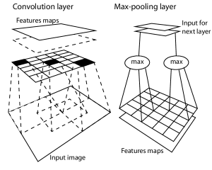
In the first layer of the CNN, the input image is fed to groups of neurons with shared weights. We scan the input image with a sliding window to get a set of sub-images. The neurons with shared weights each look at one of these sub-images and become active if certain feature as defined by the shared weights is detected from it. The different groups of neurons are used to detect different features. This process can also be viewed as convolving the input image with a set of small image kernels, or features, and then applying the hyperbolic tangent activation function to form a set of feature maps. Specifically, the feature map is given by
| (3) |
where is the feature kernel, is the input image, and is a bias term. The number of kernels, , is a free parameter in the system, and it determines the richness in the representation of the data. The second layer of the CNN is a max-pooling process. This is a form of down-sampling which bins the 2D feature maps and chooses the maximum value within each bin. The main advantage is a reduction in computational complexity in subsequent layers, though pooling also has the advantage of introducing translation invariance of the feature across the bin (Boureau et al. 2010). These two steps are illustrated in Figure 4.
The output of the max-pooling layer is fed into another convolution layer for feature detection and yet another max-pooling layer. This output is fed into the fifth and final layer, a traditional, fully-connected ANN. While the previous four layers function to locate small-scale features across the input images, the final layer combines this information to detect large-scale features and develop a global understanding of the original image.
The CNN configurations for both the time-versus-phase plot and frequency-versus-phase plot were the same. In the first step (Figure 4 left panel), both CNNs take input images down-sampled to 4848 pixels, convolve them with 20 different 1616 image kernels, producing 20 feature maps of size 3333. The subsequent max-pooling layer (Figure 4 right panel) divides each map into 33 boxes and compresses the convolved image to a size 1111 by taking the maximum in each box. The second convolution layer convolves 50 8 image kernels shared across the 20 feature maps, resulting in 50 different 44 feature maps. A second 22 max-pooling layer further compresses each feature map to an images of size 22. The result is an array of 504 numbers characterizing the local, kernel-sized features of the original image. The final layer is a traditional, fully-connected artificial neural network consisting of 500 hidden logistic units which take these 200 numbers to compute one final score.
There are 8820 artificial neurons distributed through the five layers of the CNN including the ones in the image kernels. All neurons in this network are hyperbolic tangent functions except the one that forms the final output, which is chosen to be a sigmoid function in order to map onto the classification labels 0 and 1. The training of the neural net is to let these synapses learn and store the patterns distinguishing pulsars from RFI. As an example, the last layer has weights connecting the 200 outputs of the second last layer to the 500 hidden neurons in the last layer. Each hidden neuron takes, as input, a weighted sum of the 200 outputs of the previous layer. All of the connection parameters are initialized randomly, and then updated through the process of back-propagation.
The structure of the CNN is determined by the choice of image size, kernel size, number of kernels, pooling size, and neural network size, these parameters are often called neural net design or hyper-parameters. The best CNN design, as described above, is determined through cross-validation tests. The labelled data are randomly shuffled and split into a training set formed from 60% of the candidates and a validation set from the remaining 40%, and a large grid search is performed. For each choice of design parameters the CNN is trained and the performance is characterized by computing its score (see Section 2.3) on the validation set. The CNN we used gives % when trained and tested on the time-versus-phase plots, and % for the frequency-versus-phase plots (Table 1). After optimizing the CNN design, the final AI is trained with all training candidates in order to maximize its sensitivity. The final performance of the PICS system is tested with a set of completely independent GBNCC data (see Section 3).
This CNN performs well on the frequency-versus-phase plot because a large fraction of RFI is narrow-band emission. For continuous emission this RFI shows up as a horizontal line, while burst-like or periodic RFI appears as a small dot. This is opposed to the broadband pulsed signal of a pulsar, which shows up as a vertical stripe. Since the CNN excels at detecting small-scale features, it can easily detect this form of RFI. A second reason this classifier is the best discriminant of pulsars is simply because there is more information in the 2D plots than the 1D plots. For similar reasons, the algorithm can recognize and reject burst-like RFI or signals that drift around in phase using the time-versus-phase plot.
This deep neural net is implemented using Theano (Bergstra et al. 2010), a computation library for python which compiles numerical expressions to run efficiently on either CPU or GPU architectures.
3 Results
We trained the PICS AI system with 3756 labelled PALFA candidates, among them 1659 are pulsars and their harmonics and 2097 are non-pulsars. There are only a few thousand known pulsar/harmonic candidates in PALFA but millions of non-pulsars. We picked similar numbers of pulsars and non-pulsars from the PALFA candidate pool as classified by other human experts. The pulsar candidates include unique pulsars and also the same pulsar with different beam offsets. To ensure that the AI is sensitive to both pulsars and their harmonics, % of the training pulsar candidates are harmonics of known pulsars.
We also manually rated how “pulsar-like” is each of the four subplots for every training candidate regardless of the candidate’s nature. This is because some RFI candidates may have a good pulse profile or DM curve, and we want to train the AI to recognize those the good subplots even when the candidate itself is not a pulsar. The first layer classifiers are designed to recognize patterns in individual subplot in the diagnostic plots of the candidates. Therefore they are trained to predict the “ratings” of the subplots for the training candidates, not to predict the classification of the candidates. In contrast, the second layer (LR) classifier is designed to predict whether or not a candidate is a pulsar based on the output from the first layer classifiers. Thus, it is trained with the classifications of the candidates, not with “ratings” of their subplots.
To ensure that the trained classifiers can work on new data and to determine their best initial parameters, we performed standard cross-validation tests (Section 2.5). We shuffled and split the 3756 candidates into two groups, 60% for training and 40% for validating. Furthermore, we repeated this shuffle, split, train and validate procedure 10 times to make sure their performance on validation data is reliable and repeatable. The individual first-layer classifiers score in the range 86–94% (with less than 1% RMS each) on the validation data (Table 1). The second layer of PICS, a LR algorithm that combines the scores from first-layer classifiers to form a consensus vote, scored an average of 96% (8% misses, 1% false positives) on the validation data.
To further measure the AI’s performance and determine whether it can be generalized to other surveys, we applied it to a large set of GBNCC candidates that was never seen by the AI system during training. Like PALFA, the GBNCC survey uses the PRESTO search pipeline and generates candidates in pfd format, but this survey was conducted using the Robert C. Byrd Green Bank Telescope (GBT) instead of Arecibo, so the RFI environments of the two surveys are expected to be different; furthermore, GBNCC survey uses the 350 MHz receiver instead of the 1400 MHz one, thus the DM curves of the GBNCC candidates are expected to be slightly sharper than that of the PALFA candidates thanks to the more significant dispersion effect in the lower frequency band. We applied the AI to 90008 manually labelled GBNCC candidates. An initial test showed that the AI can sort all 56 pulsars in this data set to the top 3.8%, and 68% of the pulsars to the top 0.16%. The first RFI appeared in rank 136, following 29 pulsars and 106 harmonics.
An inspection of the false positive candidates revealed many to be harmonics of the 60 Hz power signal (see Figure 6 for an example). Table 2 lists the 6 most-populous frequency ranges in a frequency histogram of all candidates, the majority of these candidates are likely caused by the 60 Hz power supply. Although these frequencies comprise 1% of the frequency domain searched by PRESTO, 24519 (roughly 27%) of the candidates fall into these frequency ranges. It is standard practice to remove harmonics of 60 Hz for North American surveys; in spite of these efforts, a significant amount of such RFI remains. Using the image patterns in the diagnostic plots, our AI was able to reject majority (%) of this RFI, with the remaining false positives strongly resembling pulsars (see Figure 6 for an example).
In light of this observation, we adjusted the scores of all candidates using a Bayesian prior on the pulse frequency to reduce the score for the false-positive candidates in contaminated frequency bins:
| (4) |
Here is the probability of being a pulsar as previously scored by PICS, , while and are the probability density functions, or likelihoods, of RFI and pulsars in frequency. can be well-approximated by sampling the frequency distribution of all test candidates, which is dominated by non-pulsar signals, especially those at 60 Hz and its harmonics (Table 2). We approximate the prior distribution by median-filtering , which removes spikes caused by RFI and leaves a distribution that reflects the survey sensitivity. At the harmonics of 60 Hz , such that , and the AI score is reduced. Away from the few affected frequency bins (Table 2), and the AI score is lightly affected, with .
The frequencies of the test candidates are binned from 0 Hz to 2000 Hz in steps of 0.5 Hz. Due to the limited bin size, all slow pulsars (1 Hz) are binned to the lowest two bins, along with a lot of RFI. Since the underlying structure of the prior distributions is not properly resolved in this domain, we did not apply the Bayesian rules to candidates with 1 Hz.
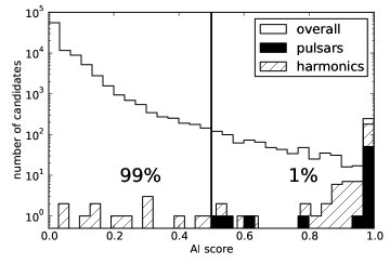
Figure 5 shows the distribution of GBNCC test candidates when sorted by , and summarizes the performance of PICS. After applying the Bayesian rule (Equation (4)), all 56 pulsars and 208 of the 221 harmonics were sorted and placed into the top 961 (1%) of the 90008 candidates by the PICS system. The first RFI candidate appeared rank 187, following 45 pulsars and 141 harmonics. The 13 harmonic candidates that were not sifted to the top are mostly candidates with very low SNR and broad profile.
A blind cross-validation test was performed using pulsars and RFI candidates collected from the PALFA survey but never seen by the AI. We found that the same Bayesian rule (Equation (4)) that worked for the GBNCC test also clearly reduced the false positive rate in this cross-validation test. This indicates that the Bayesian rule can be generalized to surveys other than GBNCC. Caution must be advised, though, since a weak pulsar candidate falling in an RFI-contaminated frequency bin (Table 2) will be down-weighted by the Bayesian prior and could be rejected. Fortunately, the chance of this happening is very small, since only a few frequency bins (%, Table 2) are affected significantly by the prior. In light of this, the Bayesian-rule RFI rejection is included only as an option in PICS and can be turned off.
Despite the size and complexity of PICS, candidate classification is a fast process because most of the individual classifiers simply apply dot products. The hard part of the computation was already done during the training phase. It took minutes to classify the 90008 GBNCC candidates using a cluster of 24 2.7GHz CPUs, 0.7 CPU second per candidate, though most of the time was spent on disk I/O and not all CPUs were used at 100% capacity. Using the same computer cluster, the AI would be able to classify a million candidates in several hours.
The PICS AI has been integrated into the PALFA pipeline, such that we can query and sort candidates using the AI rating on the cyberska.org web platform. With the help of the AI, we have found many promising candidates over several weeks, six of which have been confirmed as new PALFA discoveries. Here we list the discovery parameters of these pulsars:
-
•
PSR J1914+08 (Figure 2) is a 146.68 ms pulsar with a DM of 289 pc/cm3.
-
•
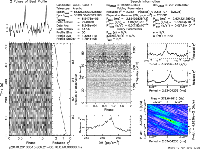
PSR J1938+20 (Figure 7) is a 2.634 ms MSP with a DM of 237 pc/cm3.
-
•
PSR J1901+02 is a 885.24 ms pulsar with a DM of 403 pc/cm3.
-
•
PSR J1903+04 is a 1151.39 ms pulsar with a DM of 473 pc/cm3
-
•
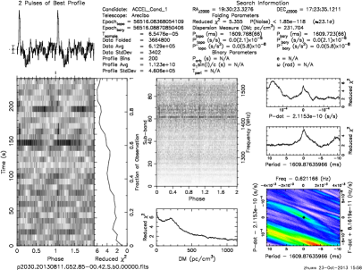
PSR J1930+17 (Figure 8) is a 1609.72 ms pulsar with a DM of 232 pc/cm3
-
•
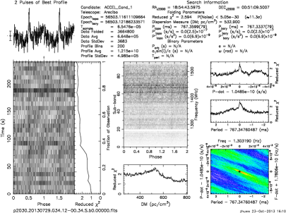
PSR J1854+00 (Figure 9) is a 767.334s pulsar with a DM of 533 pc/cm3
These pulsars are now the subject of on-going timing observations by Arecibo or Jodrell Bank Observatories.
4 Discussion
PICS scores the candidates with a number between 0 and 1, a higher score corresponding to a more pulsar-like candidate. When tested with the GBNCC data, the AI placed 100% of the pulsars and 94% of the harmonics in the top 1% (Figure 5) of ranked candidates. By rejecting 99% of the candidates, PICS can improve the speed of the candidate classification process for a human expert by a factor of 100. If we combine the AI with other ratings or scores such as the signal-to-noise ratio, the sorting efficiency can be further improved, making it possible for a few human experts to sift through millions of candidates. Such a system can be very useful for existing and future pulsar surveys.
In the GBNCC test, PICS AI showed very good performance. However, in the top 1% of the test candidates, there were still a few pulsars ranked below hundreds of non-pulsars. These were pulsars with broad pulses and low signal-to-noise ratios, and were surpassed by some strong RFI signals that also have broad features. It seems that the PICS AI could benefit from training with more pulsar/RFI training candidates that have broad pulse profiles.
Despite being limited by the quantity and diversity of the training data, the use of image-pattern-based machine learning in PICS is a novel idea and has some advantages:
The AI uses an ensemble of ML algorithms, including a deep neural network composed of many neurons and hidden weights which have the capability to recognize subtle or complex features. By gathering more human-identified candidates from surveys, we will be able to further improve the AI system. Specifically, if a survey encounters a new kind of RFI that our system or a method based on analytical heuristics fails to reject, we can improve our AI by incorporating examples of these RFI into our training data and retrain the system. Future improvements to PICS include expanding the training set to candidates from both PALFA and GBNCC surveys, and providing input capability for survey products from other search software. Rather broadly, by increasing the pool of training candidates, we can improve the accuracy of the PICS AI.
The PICS AI makes a classification based solely on image patterns in the diagnostic plots. A caveat—and, possibly, feature—is that because these plots are re-binned and normalized to unit variance, the AI ignores the DM, period and pulse amplitude differences between different candidates. Although this lost information may be useful in some rare cases (e.g. ruling out millisecond candidates with high DM based on the DM smearing timescale), this procedure forces PICS to learn the universal features of pulsars (broadband, pulsed and dispersed emission) and helps it adapt to other surveys for which sensitivity in candidate DM, frequency, and signal strength may differ. PICS is also forced to rely less on information than other score-based systems rely on, making it a good complement to them.
Being trained with many harmonic candidates with weak or multi-peak pulse profiles, the PICS AI is also very good at finding such candidates. PICS has discovered six new pulsars since being integrated into the PALFA survey pipeline. PSR J1938+20 was discovered as a very weak candidate ( according to the version of PRESTO in the PALFA pipeline at the time of discovery; Figure 7). This makes it the least significant pulsar candidate confirmed by the PALFA survey. Such a candidate probably would not have been found by a candidate-sorting method based on the significance of the signal. PSR J1914+08 was discovered as a multi-peaked harmonic, not as a candidate at its fundamental frequency. Other candidate selection methods that rely on fitting the pulse profile with a single Gaussian curve would likely down-rate these harmonics. Due to the presence of strong RFI, PSR J1930+17’s DM curve (Figure 8) is significantly skewed to the left. Similarly, PSR J1854+00’s DM curve appears to be rather shallow and also slightly skewed. It is hard to characterize these atypical DM curves using simple pre-designed functional forms. But our ML system was able to recognize these DM patterns based on similar examples in the training data.
A caveat is that the current PICS AI is trained and tested with data from PALFA and GBNCC survey, both of which have short exposure times of several hundred seconds per pointing. The pulsar candidates observed by these surveys were rarely affected significantly by scintillation or binary motion. In a survey with significantly longer exposure time, scintillation would make the pulsar signal patchy and discontinuous in the 2D subplots, while binary motion may cause pulsar signals in the time-versus-phase plot to become curved, indicating acceleration. For surveys and systems exhibiting scintillation and orbital acceleration the AI will need to be retrained with suitable candidates. Alternatively, PICS could be trained from candidates generated from numerical simulation which include these effects.
Ultimately—and with enough resources—we envision a system that adaptively trains the AI and re-scores the survey candidates on the fly while human experts are classifying them. Such an “online” system will ensure portability of the AI when the RFI environment of the telescope slowly changes over time. Remarkably, owing to the nature of the ML algorithms employed, this does not require coding new heuristics to characterize any emerging forms of RFI. One of challenges in implementing an online learning system is that the training data will be very imbalanced as pulsar surveys tend to find a lot more RFI than pulsars. Lyon et al. (2013) has explored the performance of some existing online ML algorithms in dealing with imbalanced data streams from pulsar surveys and found promise in these methods. Whether PICS could be adapted into a successful online learning system will be explored in future work.
References
- Allen et al. (2013) Allen, B., et al. 2013, ApJ, 773, 91
- Bates et al. (2012) Bates, S. D., et al. 2012, MNRAS, 427, 1052
- Bergstra et al. (2010) Bergstra, J., et al. 2010, in Proceedings of the Python for Scientific Computing Conference (SciPy), oral Presentation
- Boureau et al. (2010) Boureau, Y.-L., Ponce, J., & LeCun, Y. 2010, in International Conference on Machine Learning, 111–118
- Chang & Lin (2011) Chang, C.-C., & Lin, C.-J. 2011, ACM Transactions on Intelligent Systems and Technology, 2, 27:1, software available at http://www.csie.ntu.edu.tw/~cjlin/libsvm
- Cordes & Lazio (2001) Cordes, J. M., & Lazio, T. J. W. 2001, ApJ, 549, 997
- Cordes et al. (2006) Cordes, J. M., et al. 2006, ApJ, 637, 446
- Eatough et al. (2010) Eatough, R. P., Molkenthin, N., Kramer, M., Noutsos, A., Keith, M. J., Stappers, B. W., & Lyne, A. G. 2010, MNRAS, 407, 2443
- Faulkner et al. (2004) Faulkner, A. J., et al. 2004, MNRAS, 355, 147
- Kaspi (2012) Kaspi, V. M. 2012, in American Astronomical Society Meeting Abstracts, Vol. 219, American Astronomical Society Meeting Abstracts #219, 237.12
- Keith et al. (2009) Keith, M. J., Eatough, R. P., Lyne, A. G., Kramer, M., Possenti, A., Camilo, F., & Manchester, R. N. 2009, MNRAS, 395, 837
- Knispel et al. (2013) Knispel, B., et al. 2013, ApJ, 774, 93
- Lazarus (2013) Lazarus, P. 2013, in IAU Symposium, Vol. 291, IAU Symposium, 35–40
- LeCun et al. (1998) LeCun, Y., Bottou, L., Bengio, Y., & Haffner, P. 1998, Proceedings of the IEEE,, 86(11), 2278
- Lee (2009) Lee, K. J. 2009, PhD thesis, Peking University
- Lee et al. (2013) Lee, K. J., et al. 2013, MNRAS, 433, 688
- Lorimer et al. (2007) Lorimer, D. R., Bailes, M., McLaughlin, M. A., Narkevic, D. J., & Crawford, F. 2007, Science, 318, 777
- Lynch et al. (2013) Lynch et al. 2013, in IAU Symposium, Vol. 291, IAU Symposium, 41–46
- Lyon et al. (2013) Lyon, R. J., Brooke, J. M., Knowles, J. D., & Stappers, B. W. 2013, astro-ph.IM:1307.8012
- Pedregosa et al. (2011) Pedregosa, F., et al. 2011, Journal of Machine Learning Research, 12, 2825
- Ransom (2001) Ransom, S. M. 2001, PhD thesis, Harvard University
- Ransom et al. (2002) Ransom, S. M., Eikenberry, S. S., & Middleditch, J. 2002, Astron. J., 124, 1788
- Thornton et al. (2013) Thornton, D., et al. 2013, Science, 341, 53
| classifier | feature (sizeaaThe input features were down-sampled or interpolated to a uniform size.) | nodesbbNumber of nodes in the hidden layer of the neural network (NN). For the CNNs, only the number of nodes of the last hidden layer is listed. See Section 2.5 for more details. | cc is the radius parameter for the rbf kernel function used in the SVM. The traditional SVM can only use linear boundaries to classify data. The kernel functions enable the SVM to find curved boundaries. The rbf-kernel SVM is considered a more effective classifier than the traditional SVM. | ddThe parameter controls the regulation in the ANN and the SVM. Here regulation means that the ANN or SVM tries to minimize a penalty function while finding the optimal set of internal parameters . The function is often defined as in order to penalize very large weights. | eeThe average scores of the classifiers from 10 independent trials. In each trial, we randomly shuffle our known candidates before splitting them into training and testing data, after which training is commenced. The standard deviations of the scores are 0.01. |
|---|---|---|---|---|---|
| ANN | summed profile (64) | 25 | – | 2 | 0.86 |
| SVM | summed profile (64) | – | 0.08 | 1 | 0.93 |
| CNN | time vs phase (4848) | 500 | – | 1 | 0.92 |
| SVM | time vs phase (6464)ffPCA compression was applied to prepare 2D image data only for the SVM classifiers. We compress the 6464 image into 24 PCA components. | – | 0.01 | 1 | 0.88 |
| CNN | frequency vs phase (4848) | 500 | – | 1 | 0.94 |
| SVM | frequency vs phase (6464)ffPCA compression was applied to prepare 2D image data only for the SVM classifiers. We compress the 6464 image into 24 PCA components. | – | 0.001 | 24 | 0.88 |
| ANN | DM curve (60) | 9 | – | 10 | 0.91 |
| SVM | DM curve (60) | – | 0.2 | 25 | 0.91 |
| LR | layer-one pool (8) | – | – | 0.1 | 0.96 |
| frequency range (Hz)aaThe 6 most populous frequency ranges in the histogram of candidates. | CountsbbNumber of candidates within the given frequency range. | PercentageccPercentage of candidates within the given frequency range. |
|---|---|---|
| 1819 | 2101 | 2.3% |
| 5862 | 12941 | 14.4% |
| 118121 | 4480 | 5.0% |
| 139140 | 2157 | 2.4% |
| 179181 | 1744 | 1.9% |
| 239241 | 1096 | 1.2% |