Bell violation with entangled photons, free of the coincidence-time loophole

Abstract

In a local realist world view, physical properties are defined prior to and independent of measurement, and no physical influence can propagate faster than the speed of light. Proper experimental violation of a Bell inequality would show that the world cannot be described within local realism. Such experiments usually require additional assumptions that make them vulnerable to a number of “loopholes.” A recent experiment Gius2013 violated a Bell inequality without being vulnerable to the detection (or fair-sampling) loophole, therefore not needing the fair-sampling assumption. Here we analyze the more subtle coincidence-time loophole, and propose and prove the validity of two different methods of data analysis that avoid it. Both methods are general and can be used both for pulsed and continuous-wave experiments. We apply them to demonstrate that the experiment mentioned above violates local realism without being vulnerable to the coincidence-time loophole, therefore not needing the corresponding fair-coincidence assumption.

When attempting to provide a conclusive answer to the question by Einstein, Podolsky, and Rosen (EPR), “Can [the] quantum-mechanical description of physical reality be considered complete?” Eins1935 , it is important that assumptions concerning the physical reality are kept to an absolute minimum.

The usual assumptions underlying Bell inequalities are those of local realism — namely that properties of physical systems are elements of reality, and that these cannot be influenced faster than the speed of light; and freedom of choice — namely that the measurement setting choices are independent of the hidden variables and vice versa Bell1964 ; Bell1990 . However, all experimental demonstrations that attempt to violate a Bell inequality to date have needed additional assumptions in order to claim the invalidity of local realism. In principle, such a violation could be caused by the failure of these additional assumptions, rather than the more fundamental assumptions of local realism.

In experiments involving photons, a well known problem is that not all photons emitted by the source actually are registered in the detectors. The problem is usually referred to as the “fair-sampling” or “detection” or “detector-efficiency” loophole but really concerns the efficiency of the entire experimental setup, since there can be various causes for missing detections. The outcomes that are registered might display correlations that violate the Bell inequality even though the experiment can be described by a local realist model Pear1970 . The “fair-sampling” assumption is often used in this situation, often motivated by the assumption that successful photon detection depends only on the hidden variable and not the measurement setting. Fair sampling means that the observed outcomes of detected photons faithfully reproduce the outcome statistics of all emitted photons, if they all had been detected. This assumption is not needed in high-efficiency experiments using, e.g., atoms or superconducting qubits Rowe2001 ; Ansm2009 and the detector-efficiency loophole has only recently been avoided in photonic violations of the Clauser-Horne (CH) inequality Clau1974 (or Eberhard inequality Eber1993 ), which do not require the fair-sampling assumption Gius2013 ; Chri2013 .

Other common assumptions include “locality” Aspe1982 ; Weih1998 and “freedom of choice” Sche2010 ; assumptions may also refer to properties of decaying systems Hies2012 or properties of photons Fran1989 ; Aert1999 , and the list continues. Any of these makes an experiment vulnerable to explanation by a local realist model. Avoiding all these assumptions simultaneously in one experiment — usually called a “loophole-free” or “definitive” Bell test — remains an open task.

One less-known but equally serious problem is that of identifying which outcomes belong together Lars2004 , sometimes referred to as the “coincidence-time” loophole. Both the EPR paradox and the Bell inequality concern pairs of outcomes at two remote sites. In an experiment, it is therefore necessary to identify which outcomes make up a pair, which may be a non-trivial task. Commonly, in photon experiments, relative timing is used to identify pairs: if two clicks are close in time they are “coincident,” otherwise they are not. The problem of pair identification is especially pronounced in continuously pumped photonic experiments, but is in principle present in all experiments that have rapid repetition in the same physical system.

In this situation, it may happen that some pairs are not identified correctly. For example, if the detector jitter is large and the coincidence window small, some pairs will not register as coincident. Loss of coincidences would reduce the subset of registered pairs, and the remaining coincidences might display correlations that enable a Bell violation even though the experiment can be described by a local realist model Lars2004 . When coincidences are lost, a “fair-coincidence” assumption is needed: that the observed outcomes of all identified pairs faithfully reproduce the outcome statistics of all detected pairs of photons, if they all had been correctly identified. This can be motivated by the assumption that the time of an individual photon detection depends only on the hidden variable, and not the measurement setting.

Historically, only the fair-sampling assumption has been explicitly made, and identification of pairs within the available measurement data has not been thought of as a problem. In fact, until 2003-2004 Lars2004 , it was thought to be trivially true that coincidence determination, or timing, had no detrimental effect on Bell tests of local realism whatsoever. But since this is not the case, the fair-coincidence assumption must have been tacitly made in every experiment to date, with only a few recent exceptions Ague2012 ; Chri2013 . Here, we will provide a proof that the continuously pumped experiment Gius2013 also does not need the fair-coincidence assumption, since it is actually not vulnerable to the loophole.

The remainder of this note will I) be a more complete description of the coincidence-time loophole and how to avoid it, followed by II) an analysis of the data from Gius2013 showing that there indeed is a violation of local realism, free of the fair-coincidence assumption.

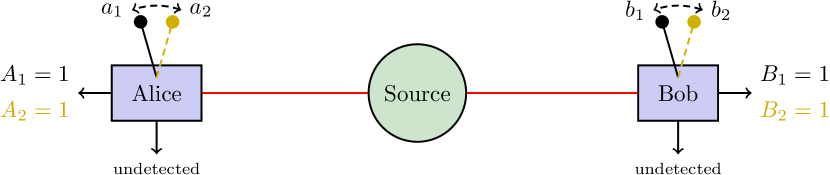
Figure 1: Principle of the experiment. Violation of the Clauser-Horne inequality needs an EPR (Einstein, Podolsky, Rosen) source of entangled pairs and two-setting measurement devices. Here, polarization entanglement and measurement is used. Each measurement device can rotate the photon’s polarization according to one of two settings ($a_{1}$ or $a_{2}$ and $b_{1}$ or $b_{2}$) before checking if a photon arrives at the “ordinary” output of a polarizing beam splitter. This is recorded as the event $A_{1}=1$, $A_{2}=1$, $B_{1}=1$ or $B_{2}=1$, depending on site and setting, as appropriate.

Avoiding the coincidence-time loophole — In a typical Bell-type experiment based on photon pairs (see Fig. 1), the usual way to determine if two events belong to the same pair is to compare the two detection times and conclude that a coincidence has happened if the two times are close. More precisely, there is a coincidence for setting $a\in\{a_{1},a_{2}\}$ at the first site (Alice) and $b\in\{b_{1},b_{2}\}$ at the second (Bob) if their detection times $T_{A}$ and $T_{B}$ are close enough so that

$$\big{|}T_{A}(a)-T_{B}(b)\big{|}<\tfrac{1}{2}\tau.$$ (1)

Here, the chosen coincidence window width $\tau$ is the total possible deviation in a detection time at one site, given the detection time at the other. To the experimentalist, this is the event “there is a coincidence,” and the probability of such an event is well-defined even without reference to hidden variables (see Fig. 2a).

In a local realist model, the detection times $T_{A}$ and $T_{B}$ at the two sites would be random variables that depend on the local settings $a$ and $b$, with the hidden variable $\lambda$ as argument: $T_{A}(a,\lambda)$, and $T_{B}(b,\lambda)$. Here, the locality assumption ensures that the detection times do not depend on the remote setting, just as is assumed for the outcomes. Coincidences (of outcomes $A\in\{A_{1},A_{2}\}$ for Alice and $B\in\{B_{1},B_{2}\}$ for Bob, where the subscript denotes the setting used for measurement) now occur on a subset of the hidden-variable space that can be written as

$$\Lambda_{A_{j}B_{k}}=\big{\{}\lambda:\big{|}T_{A}(a_{j},\lambda)-T_{B}(b_{k},\lambda)\big{|}<\tfrac{1}{2}\tau\big{\}},$$ (2)

with $j,k=1,2$. This is the mathematical, or rather, the probabilistic formalization of the coincidence event, and the mathematical term for such a subset of the sample space is “event.”

The structure of the above coincidence set is very different from the structure of the set of coincidences when only missing outcomes (and possibly unfair sampling) are taken into account. If clicks occur on the sets $\Lambda_{A_{j}}$ and $\Lambda_{B_{k}}$, and all coincidences are correctly identified, the coincidence set has the factorizable structure

$$\Lambda_{A_{j}B_{k}}=\Lambda_{A_{j}}\cap\Lambda_{B_{k}}.$$ (3)

This leads to an experimental efficiency requirement of at least $\approx$ $82.84\%$ to achieve a violation of local realism (in the Clauser-Horne-Shimony-Holt Clau1969 inequality) free of the fair-sampling assumption. Because the set (2) cannot be factored, the bound to avoid the fair-coincidence assumption will be higher, $\approx$ $87.87\%$ Lars2004 .

In this note, we are interested in the Clauser-Horne (CH) inequality, which holds under the assumptions of realism, locality, and freedom of choice;

$$P (A_{1}=B_{2}=1)+P(A_{2}=B_{1}=1)-P(A_{2}=B_{2}=1)$$

$$\leq P(A_{1}=1)+P(B_{1}=1)-P(A_{1}=B_{1}=1).$$ (4)

See the Methods section for formal definitions and proofs.

This inequality avoids the detector-efficiency loophole so that experimental violation does not need the fair-sampling assumption. However, it does not take into account how pairs are identified, e.g., how coincidences are determined by timing data in the experimental output. We would want to establish a similar inequality that includes restricting to a subset of pairs, $P(A_{j}=B_{k}=1\cap\Lambda_{A_{j}B_{k}})$, and detection, e.g., $P(A_{j}=1\cap\Lambda_{A_{j}})$. Fortunately, this is not too difficult.

There are two alternative methods. The first uses fixed non-overlapping time slots,

$$S_{i}=\big{\{}t:t_{i}\leq t<t_{i}+\tau\big{\}},$$ (5)

for detection and coincidence determination (we use the same $\tau$ for time slot size and time window size because that gives a similar rate of accidental coincidences, making the two methods easily comparable). This enables a CH-type inequality that avoids the coincidence-time loophole, making experiments that use the new inequality independent of the fair-coincidence assumption. The reason is that a fixed time slot border treats long and short delays equally, see Fig. 2b. In pulsed photonic experiments, there is a natural time slot structure because of the pulse timing. However, also for continuously pumped experiments fixed time slots for coincidence identification can be easily enforced.

A detection is only counted if it occurs in one of the time slots, in a local realist model corresponding to

$$\begin{split}\Lambda_{A_{j}}(i)=\big{\{}\lambda:T_{A}(a_{j},\lambda)\in S_{i}\big{\}},\\ \Lambda_{B_{k}}(i)=\big{\{}\lambda:T_{B}(b_{k},\lambda)\in S_{i}\big{\}},\end{split}$$ (6)

and for all the time slots we have the disjoint union

$$\Lambda_{A_{j}}=\bigcup_{i}\Lambda_{A_{j}}(i),$$ (7)

and similar for $\Lambda_{B_{k}}$. A coincidence occurs in slot $i$ if both detections occur there, and this happens on the set $\Lambda_{A_{j}}(i)\cap\Lambda_{B_{k}}(i)$. A coincidence in any slot occurs on the disjoint union

$$\Lambda_{A_{j}B_{k}}=\bigcup_{i}\Big{(}\Lambda_{A_{j}}(i)\cap\Lambda_{B_{k}}(i)\Big{)}.$$ (8)

This is not the factor structure we have in the detector efficiency case, but it will enable us to recover the appropriate inequality. It is important that time slots are assigned locally, so that no remote influence is present; such influence would result in a set structure similar to that in Eq. (2). We can now include coincidence determination in the inequality, and arrive at

$$P (A_{1}=B_{2}=1\;\cap\;\Lambda_{A_{1}B_{2}})+P(A_{2}=B_{1}=1\;\cap\;\Lambda_{A_{2}B_{1}})$$

$$\quad-P(A_{2}=B_{2}=1\;\cap\;\Lambda_{A_{2}B_{2}})$$

$$\leq P(A_{1}=1\;\cap\;\Lambda_{A_{1}})+P(B_{1}=1\;\cap\;\Lambda_{B_{1}})$$

$$\quad-P(A_{1}=B_{1}=1\;\cap\;\Lambda_{A_{1}B_{1}}).$$ (9)

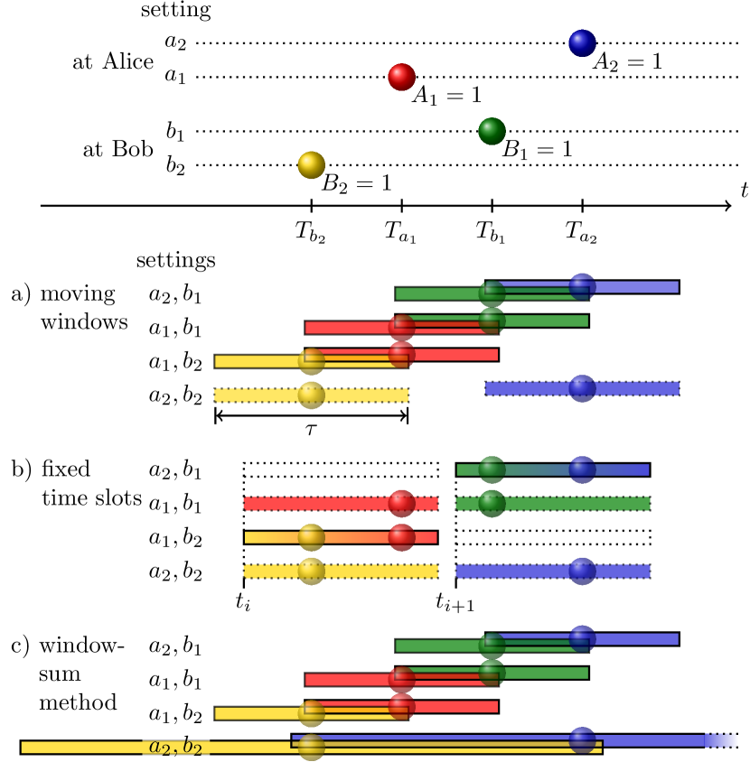
Figure 2: Comparison of the three different methods to identify coincidences. At the top is an example of a possible assignment to the detection times for a given $\lambda$, chosen to illustrate the key features of the different pair identification methods. In method a), a coincidence is identified if detection times are close enough (with difference of at most half the coincidence window $\tau$), here for settings $a_{2},b_{1}$; $a_{1},b_{1}$; and $a_{1},b_{2}$ but not for $a_{2},b_{2}$. The $a_{2},b_{2}$ events would then be misidentified as not being coincident. The fair-coincidence assumption implies that this, on average, happens equally often for all combinations, which is a substantial restriction on possible local realist models. Method b) uses fixed time slots of size $\tau$ to avoid the coincidence-time loophole by ensuring that if $a_{2},b_{2}$ would not give a coincidence, at least one of $a_{2},b_{1}$; $a_{1},b_{1}$; or $a_{1},b_{2}$ would also not do so (in the figure, this is $a_{1},b_{1}$). Above, the time slots are separated as is appropriate for a pulsed experiment, while adjacent slots is the best choice for a continuously pumped experiment. Method c) uses a different approach, namely a longer time window for the $a_{2},b_{2}$ settings, to ensure that if all the others ($a_{2},b_{1}$; $a_{1},b_{1}$; or $a_{1},b_{2}$) would give a coincidence, so would $a_{2},b_{2}$. The two new methods are opposite in the sense that in method b) coincidences are lost as compared to method a) while in method c) coincidences are gained; both avoid the coincidence-time loophole.

The key observation here is that the inequality avoids the coincidence-time loophole and can be properly violated by experiment, as soon as disjoint fixed time slots are used. It does not matter how the time slots are chosen (as long as they are locally assigned), or if they have a natural counterpart in the experiment. This is especially important in continuously pumped photonic experiments.

We should point out that the event $A_{j}=1$ does not necessarily mean a single click in a detector in one time slot. It is a label for some event we are interested in. In the data analysis, one can choose the event $A_{j}=1$ to correspond to at least one detection for setting $a_{j}$ at the first site, and similarly for $B_{k}=1$ (setting $b_{k}$ at the second). Note that this choice must be made entirely from the locally available information. A coincidence (the event $\Lambda_{A_{j}B_{k}}$) would then correspond to (any number of) detections in two equal-indexed time slots, using information from both sites. Operationally, this means to coarse-grain all detector clicks on each side and for every time slot to dichotomic values: “0” = “no detections,” “1” = “one or more detections.” This coarse-graining method allows no switching of settings within time slots, but this can be handled also.

The alternative method does not need fixed time slots. The intuition for this method is that all proposed local realist models that exploit the loophole put some of the $A_{2}B_{2}$ detection events more than $\tfrac{1}{2}\tau$ apart, so that they are not identified as a coincidence. It therefore makes sense to increase the window for the $A_{2}B_{2}$ events. With

$$\begin{split}\Lambda_{A_{1}B_{1}}&=\big{\{}\lambda:\big{|}T_{A}(a_{1},\lambda)-T_{B}(b_{1},\lambda)\big{|}<\tfrac{1}{2}\tau_{1}\big{\}},\\ \Lambda_{A_{1}B_{2}}&=\big{\{}\lambda:\big{|}T_{A}(a_{1},\lambda)-T_{B}(b_{2},\lambda)\big{|}<\tfrac{1}{2}\tau_{2}\big{\}},\\ \Lambda_{A_{2}B_{1}}&=\big{\{}\lambda:\big{|}T_{A}(a_{2},\lambda)-T_{B}(b_{1},\lambda)\big{|}<\tfrac{1}{2}\tau_{3}\big{\}},\\ \Lambda_{A_{2}B_{2}}&=\big{\{}\lambda:\big{|}T_{A}(a_{2},\lambda)-T_{B}(b_{2},\lambda)\big{|}<\tfrac{1}{2}\textstyle\sum_{i}\tau_{i}\big{\}},\\ \end{split}$$ (10)

we obtain

$$\Lambda_{A_{1}B_{1}}\cap\Lambda_{A_{1}B_{2}}\cap\Lambda_{A_{2}B_{1}}\;\subset\;\Lambda_{A_{2}B_{2}}.$$ (11)

In other words: if the $A_{1}B_{1}$, $A_{1}B_{2}$, and $A_{2}B_{1}$ detection events that are separated by at most $\tau_{i}$ are identified as coincidences, then the $A_{2}B_{2}$ detection events separated by at most $\sum_{i}\tau_{i}$ are also identified as coincidences (see Fig. 2c). This gives the inequality

$$P (A_{1}=B_{2}=1\;\cap\;\Lambda_{A_{1}B_{2}})+P(A_{2}=B_{1}=1\;\cap\;\Lambda_{A_{2}B_{1}})$$

$$\quad-P(A_{2}=B_{2}=1\;\cap\;\Lambda_{A_{2}B_{2}})$$

$$\leq P(A_{1}=1)+P(B_{1}=1)$$

$$\quad-P(A_{1}=B_{1}=1\;\cap\;\Lambda_{A_{1}B_{1}}).$$ (12)

We remark that, in contrast to the “fixed-time-slots method” (Fig. 2b), no coarse-graining of multiple clicks is applied in the “window-sum method” (Fig. 2c).

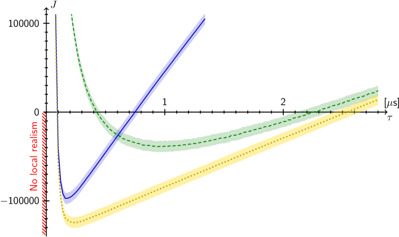
Figure 3: Experimental $J$ values plotted as a function of coincidence window or time slot size $\tau$. The three alternatives are a) the dotted yellow line that uses the moving-windows method and the fair-coincidence assumption; b) the green dashed line that uses the fixed-time-slots method; and c) the blue continuous line that uses the window-sum method (with all $\tau_{i}$ equal to $\tau$). The latter two are not vulnerable to the coincidence-time loophole. The shading corresponds to plus/minus three estimated standard deviations. Negative $J$ values cannot be explained by local realist models.

Violation from the experiment Gius2013 — The CH inequality is not vulnerable to the detector-efficiency loophole, and therefore free of the fair-sampling assumption. As shown above, similar inequalities that are not vulnerable to the coincidence-time loophole can be derived by two methods (Ineq. (Bell violation with entangled photons, free of the coincidence-time loophole) and (Bell violation with entangled photons, free of the coincidence-time loophole)), both therefore free of the fair-coincidence assumption. Both statements also hold for the Eberhard inequality, where all probabilities in the CH inequality are replaced by the corresponding number of counts. Applying the fixed-time-slots or window-sum method leads to Eberhard-type inequalities similar to Ineq. (Bell violation with entangled photons, free of the coincidence-time loophole) and (Bell violation with entangled photons, free of the coincidence-time loophole), free of the fair-coincidence assumption as well as the fair-sampling assumption. Collecting all terms on one side creates inequalities of the form

$$J\geq 0.$$ (13)

Since the fixed-time-slots method removes coincidences as compared to the moving windows method (compare Fig. 2a and Fig. 2b), it comes at a cost in a continuously pumped experiment: because of the inherently random emission times and the timing jitter of the detectors, two photons close in time that would be coincident in the moving-window method may belong to different time slots and fail to register a coincidence in the fixed-time-slots method. To minimize the loss, long adjacent slots (much longer than the timing jitter of the detectors used) are desirable, and the earlier-mentioned coarse-graining should be used because multiple generated pairs can appear in the same slot. Coarse-grained coincidences may not show quantum correlations, and can prohibit or hamper a violation of the tested Bell inequality. Therefore, depending on experimental parameters such as timing jitter, overall efficiency, background counts, and rate of generated pairs, there will be an optimal size for the locally predefined time slots, see Fig. 3b.

For the experiment Gius2013 , choosing adjacent predefined time slots with size $\tau=980$ ns, yields $J=-38803\pm 2020$. This corresponds to a violation, free of the fair-coincidence assumption, by more than $19\,\sigma$ (estimated standard deviations). The standard deviation is estimated analogously to Gius2013 , by dividing the data set into 30 subsets and using standard unbiased point estimates, adjusting these to apply to the sum of the 30 samples rather than the mean.

Finally, we also analyze the data of Ref. Gius2013 using the window-sum method (Fig. 2c and Fig. 3c) with all three $\tau_{i}$ being equal to $\tau$ and the window for $A_{2}B_{2}$ being $3\tau$. For $\tau=180$ ns, one obtains $J=-96988\pm 2076$, a $46\,\sigma$ violation (estimated standard deviations). The window-sum method typically leads to a larger violation than the fixed-time-slots method since it evades the trade-offs encountered in choosing a slot size. The only “penalty” is an increase of the accidental coincidences for the $A_{2}B_{2}$ events. Therefore, the window-sum method can be a valuable tool in situations where unfavorable experimental parameters (such as high timing jitter and dark counts of the detectors) do not allow a violation using the fixed-time-slots method.

For the above $J$ values we calculated the singles counts as follows: Alice’s singles counts for outcome $A_{1}$ were taken to be the mean of her singles when she and Bob applied settings $a_{1},b_{1}$ and when they applied $a_{1},b_{2}$. Similarly, Bob’s singles counts for outcome $B_{1}$ were taken to be the average obtained from the setting combinations $a_{1},b_{1}$ and $a_{2},b_{1}$. In an ideal experiment, the $J$ value should not depend on whether this averaging is employed or individual combinations are taken. However, due to the residual drifts discussed in Ref. Kofl2013 the above reported $J$ values for the data of Ref. Gius2013 do depend on the procedure, albeit not in any way that would alter the conclusion, namely a significant violation of CH- or Eberhard-type inequalities that are not vulnerable to the coincidence-time loophole.

Conclusion — In their original form, the CH and Eberhard inequalities are derived without using the assumption of fair sampling. Here, we have derived CH- and Eberhard-type inequalities that are also free of the coincidence-time loophole, through two different approaches. One is to use fixed time slots for the local measurement results and identify coincidences if detections occur in equal time slots, while the other is to choose a key coincidence window as long as the sum of the others. Both methods can be used in continuously pumped experiments as well as in pulsed experiments, and in particular, both can be used to show that the experiment reported in Ref. Gius2013 violates local realism and is not vulnerable to the coincidence-time loophole, therefore not needing the fair-coincidence assumption.

Methods — Realist models (or hidden variable models) are probabilistic models that use three building blocks. The first building block is a sample space $\Lambda$, which is the set of possible hidden variable values. The second is a family of event subsets $E\subset\Lambda$, e.g., the sets of hidden variable values where specific measurement outcomes occur. The third and final building block is that these event sets must be measurable using a probability measure $P$, so that each event has a well-defined probability. If the sample (hidden variable) $\lambda$ is reasonably well-behaved, its distribution $\rho$ can be constructed from this. Below, we will use deterministic realism without loss of generality, since stochastic realist models are equivalent to mixtures of deterministic ones Fine1982 . We can now prove the following theorems.

Theorem 1 (Clauser-Horne): The following three prerequisites are assumed to hold except at a null set:

1. Realism. Measurement results can be described by two families of random variables ($A$ for Alice with local setting $a$, $B$ for Bob with local setting $b$):

   $$A(a,b,\lambda)\text{ and }B(a,b,\lambda).$$ (14)

   The dependence on the hidden variable $\lambda$ is usually suppressed in the notation.

2. Locality. Measurement results are independent of the remote setting:

   $$\begin{split}A(a,\lambda)&\stackrel{{\scriptstyle\textrm{def}}}{{=}}A(a,b_{1},\lambda)=A(a,b_{2},\lambda)\\ B(b,\lambda)&\stackrel{{\scriptstyle\textrm{def}}}{{=}}B(a_{1},b,\lambda)=B(a_{2},b,\lambda).\end{split}$$ (15)

   For brevity we define $A_{j}(\lambda)=A(a_{j},\lambda)$ and $B_{k}(\lambda)=B(b_{k},\lambda)$.

3. Freedom of choice. The measurement setting distribution does not depend on the hidden variable, or equivalently, the probability measure $P$ does not depend on the measurement settings; this is sometimes formulated as independence between the distribution $\rho$ of $\lambda$ and the measurement settings,

   $$P(E|a,b)=P(E)\text{ or }\rho(\lambda|a,b)=\rho(\lambda).$$ (16)

Then,

$$P (A_{1}=B_{2}=1)+P(A_{2}=B_{1}=1)-P(A_{2}=B_{2}=1)$$

$$\leq P(A_{1}=1)+P(B_{1}=1)-P(A_{1}=B_{1}=1).$$ (17)

Proof:

$$P (A_{1}=B_{2}=1)+P(A_{2}=B_{1}=1)-P(A_{2}=B_{2}=1)$$

$$\leq P(A_{1}=B_{2}=1)+P(A_{2}=B_{1}=1)$$

$$\quad-P(A_{1}=B_{2}=1\cap A_{2}=B_{1}=1)$$

$$=P(A_{1}=B_{2}=1\;\cup\;A_{2}=B_{1}=1)$$

$$\leq P(A_{1}=1\;\cup\;B_{1}=1)$$ (18)

$$=P(A_{1}=1)+P(B_{1}=1)-P(A_{1}=B_{1}=1) \square$$

Using the notation for fixed non-overlapping time slots from the main text, we have the following theorem.

Theorem 2 (The Clauser-Horne inequality with disjoint time slots): If the prerequisites from the Clauser-Horne inequality are assumed to hold except at a null set, and also:

1. Disjoint time slots. Detections are obtained on subsets $\Lambda_{A_{j}}$; $\Lambda_{B_{k}}$ with $j,k=1,2$ of $\Lambda$ that are disjoint unions of the form

   $$\Lambda_{A_{j}}=\bigcup_{i}\Lambda_{A_{j}}(i),$$ (19)

   and coincidences are obtained on subsets $\Lambda_{A_{j}B_{k}}$ of $\Lambda$ that are disjoint unions of the form

   $$\Lambda_{A_{j}B_{k}}=\bigcup_{i}\Big{(}\Lambda_{A_{j}}(i)\cap\Lambda_{B_{k}}(i)\Big{)}.$$ (20)

Then

$$P (A_{1}=B_{2}=1\;\cap\;\Lambda_{A_{1}B_{2}})+P(A_{2}=B_{1}=1\;\cap\;\Lambda_{A_{2}B_{1}})$$

$$\quad-P(A_{2}=B_{2}=1\;\cap\;\Lambda_{A_{2}B_{2}})$$

$$\leq P(A_{1}=1\;\cap\;\Lambda_{A_{1}})+P(B_{1}=1\;\cap\;\Lambda_{B_{1}})$$

$$\quad-P(A_{1}=B_{1}=1\;\cap\;\Lambda_{A_{1}B_{1}}).$$ (21)

Proof: Define new time-slot-indexed random variables, e.g., $A_{j}^{(i)}$ that indicates that $A_{j}=1$ in time slot $i$,

$$A_{j}^{(i)}=1\quad\Leftrightarrow\quad\big{(}A_{j}=1\cap\Lambda_{A_{j}}(i)\big{)}.$$ (22)

Since the sets are disjoint unions, we have for example

$$\begin{split}P(A_{1}=1\;\cap\;\Lambda_{A_{1}})&=P\Big{(}A_{1}=1\;\cap\;\big{(}\bigcup_{i}\Lambda_{A_{1}}(i)\big{)}\Big{)}\\ &=\sum_{i}P(A_{1}^{(i)}=1),\end{split}$$ (23)

and

$$\begin{split}P&(A_{1}=B_{2}=1\;\cap\;\Lambda_{A_{1}B_{2}})\\ &=P\Big{(}A_{1}=B_{2}=1\;\cap\;\big{(}\bigcup_{i}\Lambda_{A_{1}}(i)\cap\Lambda_{B_{2}}(i)\big{)}\Big{)}\\ &=\sum_{i}P\big{(}A_{1}^{(i)}=B_{2}^{(i)}=1\big{)}.\end{split}$$ (24)

The inequality now follows from using the original CH inequality in each time slot. $\square$

Finally, for the window-sum method we have the following.

Theorem 3 (The Clauser-Horne inequality with a subset property): If the prerequisites from the Clauser-Horne inequality are assumed to hold except at a null set, and also:

1. Subset property. Coincidences are obtained on subsets $\Lambda_{A_{1}B_{1}}$; $\Lambda_{A_{1}B_{2}}$; $\Lambda_{A_{2}B_{1}}$; and $\Lambda_{A_{2}B_{2}}$, of $\Lambda$, and the last coincidence set contains the intersection of the other three,

   $$\Lambda_{A_{1}B_{1}}\cap\Lambda_{A_{1}B_{2}}\cap\Lambda_{A_{2}B_{1}}\;\subset\;\Lambda_{A_{2}B_{2}}.$$ (25)

Then

$$P (A_{1}=B_{2}=1\;\cap\;\Lambda_{A_{1}B_{2}})+P(A_{2}=B_{1}=1\;\cap\;\Lambda_{A_{2}B_{1}})$$

$$\quad-P(A_{2}=B_{2}=1\;\cap\;\Lambda_{A_{2}B_{2}})$$

$$\leq P(A_{1}=1)+P(B_{1}=1)$$

$$\quad-P(A_{1}=B_{1}=1\;\cap\;\Lambda_{A_{1}B_{1}}).$$ (26)

Proof: We need to treat the $A_{2}B_{2}$ events separately,

$$\begin{split}&P(A_{2}=B_{2}=1\;\cap\;\Lambda_{A_{2}B_{2}})\\ &\;\geq P(A_{2}=B_{2}=1\;\cap\;\Lambda_{A_{1}B_{1}}\cap\Lambda_{A_{1}B_{2}}\cap\Lambda_{A_{2}B_{1}})\\ &\;\geq P\Big{(}\big{(}(A_{1}=B_{2}=1\cap\Lambda_{A_{1}B_{2}})\\ &\qquad\quad\cap(A_{2}=B_{1}=1\cap\Lambda_{A_{2}B_{1}})\big{)}\cap\Lambda_{A_{1}B_{1}}\Big{)}.\end{split}$$ (27)

The proof of Theorem 1 now applies on the subset $\Lambda_{A_{1}B_{1}}$ so that

$$\begin{split}P&(A_{1}=B_{2}=1\;\cap\;\Lambda_{A_{1}B_{2}}\cap\Lambda_{A_{1}B_{1}})\\ &\quad+P(A_{2}=B_{1}=1\;\cap\;\Lambda_{A_{2}B_{1}}\cap\Lambda_{A_{1}B_{1}})\\ &\quad-P(A_{2}=B_{2}=1\;\cap\;\Lambda_{A_{2}B_{2}})\\ &\leq P(A_{1}=1\cap\Lambda_{A_{1}B_{1}})+P(V_{1}=1\cap\Lambda_{A_{1}B_{1}})\\ &\quad-P(A_{1}=B_{1}=1\;\cap\;\Lambda_{A_{1}B_{1}}).\end{split}$$ (28)

Since

$$\begin{split}P&(A_{1}\!=\!B_{2}\!=\!1\cap\Lambda_{A_{1}B_{2}}\setminus\Lambda_{A_{1}B_{1}})\leq P(A_{1}\!=\!1\setminus\Lambda_{A_{1}B_{1}}),\\ P&(A_{2}\!=\!B_{1}\!=\!1\cap\Lambda_{A_{2}B_{1}}\setminus\Lambda_{A_{1}B_{1}})\leq P(B_{1}\!=\!1\setminus\Lambda_{A_{1}B_{1}}),\end{split}$$ (29)

the result follows. $\square$

Note added — During the preparation of this manuscript it has come to our attention that the window-sum method has been discovered independently by Emanuel Knill and co-workers in the context of an extended statistical analyis Knil2013 .

Acknowledgments — We would like to acknowledge discussions with Anton Zeilinger, Sae Woo Nam, and Emanuel Knill; and assistance with the detection system from Alexandra Mech, Jörn Beyer, Adriana Lita, Brice Calkins, Thomas Gerrits, and Sae Woo Nam. SR is supported by an EU Marie-Curie Fellowship (PIOF-GA-2012-329851).

References

- (1) M. Giustina, A. Mech, S. Ramelow, B. Wittmann, J. Kofler, J. Beyer, A. Lita, B. Calkins, T. Gerrits, S.W. Nam, R. Ursin, and A. Zeilinger, Nature 497, 227 (2013).
- (2) A. Einstein, B. Podolsky, and N. Rosen, Phys. Rev. 47, 777 (1935).
- (3) J. S. Bell, Physics (New York) 1, 195 (1964).
- (4) J. S. Bell, “La nouvelle cuisine”, chapter 6 of Between Science and Technology, editors A. Sarlemijn and P. Kroes, Elsevier Science Publishers (1990); reprinted in J. S. Bell, Speakable and Unspeakable in Quantum Mechanics, 2nd ed., pp. 232–248, Cambridge University Press, UK, (2004)
- (5) P. M. Pearle, Phys. Rev. D 2, 1418 (1970).
- (6) M. A. Rowe, D. Kielpinski, V. Meyer, C. A. Sackett, W. M. Itano, C. Monroe, and D. J. Wineland, Nature 409, 791 (2001).
- (7) M. Ansmann, H. Wang, R. C. Bialczak, M. Hofheinz, E. Lucero, M. Neeley, A. D. O’Connell, D. Sank, M. Weides, J. Wenner, A. N. Cleland, and J. M. Martinis, Nature 461, 504 (2009).
- (8) J. F. Clauser and M. A. Horne, Phys. Rev. D 10, 526 (1974).
- (9) P. H. Eberhard, Phys. Rev. A 47, 747 (1993).
- (10) B. G. Christensen, K. T. McCusker, J. Altepeter, B. Calkins, T. Gerrits, A. E. Lita, A. Miller, L. K. Shalm, Y. Zhang, S. W. Nam, N. Brunner, C. C. W. Lim, N. Gisin, and P. G. Kwiat, Phys. Rev. Lett. 111, 130406 (2013).
- (11) A. Aspect, J. Dalibard, and G. Roger, Phys. Rev. Lett. 49, 1804 (1982).
- (12) G. Weihs, T. Jennewein, C. Simon, H. Weinfurter, and A. Zeilinger, Phys. Rev. Lett. 81, 5039 (1998).
- (13) T. Scheidl, R. Ursin, J. Kofler, S. Ramelow, X.-S. Ma, T. Herbst, L. Ratschbacher, A. Fedrizzi, N.K. Langford, T. Jennewein, and A. Zeilinger, Proc. Natl. Acad. Sci. USA 107, 19708 (2010).
- (14) B. C. Hiesmayr, A. Di Domenico, C. Curceanu, A. Gabriel, M. Huber, J.-Å. Larsson, P. Moskal, Eur. Phys. J. C 72, 1856 (2012).
- (15) J. D. Franson, Phys. Rev. Lett. 62, 2205 (1989).
- (16) S. Aerts, P. Kwiat, J.-Å. Larsson, M. Zukowski, Phys. Rev. Lett., 83, 2872 (1999).
- (17) J.-Å. Larsson and R. D. Gill, Europhys. Lett. 67, 707 (2004).
- (18) M. B. Agüero, A. A. Hnilo, and M. G. Kovalsky, Phys. Rev. A 86, 052121 (2012).
- (19) J. F. Clauser, M. A. Horne, A. Shimony, and R. A. Holt, Phys. Rev. Lett. 23, 880 (1969).
- (20) A. Fine, Phys. Rev. Lett. 48, 291 (1982).
- (21) J. Kofler, S. Ramelow, M. Giustina, and A. Zeilinger, arXiv:1307.6475 [quant-ph].
- (22) E. Knill, S. W. Nam, S. Glancy, Y. Zhang, private comm.