NASA Kepler Mission White Paper

Asteroseismology of Solar-Like Oscillators in a 2-Wheel Mission

W. J Chaplin^1,2, H. Kjeldsen², J. Christensen-Dalsgaard², R. L. Gilliland³, S. D. Kawaler⁴, S. Basu⁵, J. De Ridder⁶, D. Huber⁷, T. Arentoft², J. Schou⁸, R. A. García⁹, T. S. Metcalfe^10,2, K. Brogaard², T. L. Campante^1,2, Y. Elsworth^1,2, A. Miglio^1,2, T. Appourchaux¹¹, T. R. Bedding¹², S. Hekker⁸, G. Houdek², C. Karoff², J. Molenda-Żakowicz¹³, M. J. P. F. G. Monteiro¹⁴, V. Silva Aguirre², D. Stello¹², W. Ball¹⁵, P. G. Beck⁶, A. C. Birch⁸, D. L. Buzasi¹⁶, L. Casagrande¹⁷, T. Cellier⁹, E. Corsaro⁶, O. L. Creevey¹¹, G. R. Davies^1,2, S. Deheuvels¹⁸, G. Doğan^19,2, L. Gizon^8,15, F. Grundahl², J. Guzik²⁰, R. Handberg^1,2, A. Jiménez²¹, T. Kallinger²², M. N. Lund², M. Lundkvist², S. Mathis⁹, S. Mathur¹⁰, A. Mazumdar²³, B. Mosser²⁴, C. Neiner²⁴, M. B. Nielsen¹⁵, P. L. Pallé²¹, M. H. Pinsonneault²⁵, D. Salabert⁹, A. M. Serenelli²⁶, H. Shunker⁸, T. R. White^15,12

(1) Univ. of Birmingham, UK (2) Stellar Astrophysics Centre, Aarhus Univ., Denmark (3) Pennsylvania State Univ., USA (4) Iowa State Univ., USA (5) Yale Univ., USA (6) K.U. Leuven, Belgium (7) NASA Ames Research Center, USA (8) Max Planck Institute for Solar System Research, Germany (9) CEA/DSM-CNRS-Univ. Paris Diderot, France (10) Space Science Institute, USA (11) Univ. Paris-Sud, Institut d’Astrophysique Spatiale, France (12) Univ. of Sydney, Australia (13) University of Wrocław, Poland (14) Univ. do Porto, Portugal (15) Univ. of Goettingen, Germany (16) Florida Gulf Coast Univ., USA (17) The Australian National Univ., Australia (18) Univ. de Toulouse, France (19) HAO, Boulder, USA (20) Los Alamos National Laboratory, USA (21) IAC, Tenerife, Spain (22) Univ. of Vienna, Austria (23) Homi Bhabha Centre for Science Education, India (24) Observatoire de Paris, France (25) Ohio State Univ., USA (26) Institute of Space Sciences (IEEC-CSIC), Spain

Abstract

This document is a response to the Kepler Project Call for White Papers. In it, we comment on the potential for continuing asteroseismology of solar-type and red-giant stars in a 2-wheel Kepler Mission. These stars show rich spectra of solar-like oscillations. Our main conclusion is that by targeting stars in the ecliptic it should be possible to perform high-quality asteroseismology, as long as favorable scenarios for 2-wheel pointing performance are met. Targeting the ecliptic would potentially facilitate unique science that was not possible in the nominal Mission, notably from the study of clusters that are significantly brighter than those in the Kepler field.

Our conclusions are based on predictions of 2-wheel observations made by a space photometry simulator, with information provided by the Kepler Project used as input to describe the degraded pointing scenarios. We find that elevated levels of frequency-dependent noise, consistent with the above scenarios, would have a significant negative impact on our ability to continue asteroseismic studies of solar-like oscillators in the Kepler field. However, the situation may be much more optimistic for observations in the ecliptic, provided that pointing resets of the spacecraft during regular desaturations of the two functioning reaction wheels are accurate at the $\leq 1\,\rm arcsec$ level. This would make it possible to apply a post-hoc analysis that would recover most of the lost photometric precision. Without this post-hoc correction—and the accurate re-pointing it requires—the performance would probably be as poor as in the Kepler-field case. Critical to our conclusions for both fields is the assumed level of pointing noise (in the short-term jitter and the longer-term drift). We suggest that further tests will be needed to clarify our results once more detail and data on the expected pointing performance becomes available, and we offer our assistance in this work.

1 Introduction

1.1 Results from Kepler

Asteroseismology has been one of the major successes of Kepler. The research has been conducted in the framework of the Kepler Asteroseismic Science Consortium (KASC; Gilliland et al. 2010). Kepler has provided data of exquisite quality for the asteroseismic study of unprecedented numbers of low-mass main-sequence stars and cool subgiants (Chaplin et al. 2011a) and red giants (e.g., Bedding et al. 2011; Hekker et al., 2011; Huber et al. 2011; Kallinger et al., 2012; Mosser et al. 2012a; Stello et al. 2013), including red giants in open clusters (e.g., Basu et al. 2010; Stello et al. 2010; Corsaro et al. 2012; Miglio et al. 2012). These stars show rich spectra of overtones of radial and non-radial solar-like oscillations, pulsations that are stochastically excited and intrinsically damped by near-surface convection. The Kepler data have provided a unique combination of extremely high-quality photometry and continuous, long-term coverage lasting up to several years for many stars. Long, high-duty-cycle lightcurves provide the frequency resolution needed to measure the frequencies, frequency splittings (from rotation and magnetic fields), and other parameters of individual modes. These parameters allow estimation of fundamental stellar properties (e.g., see Metcalfe et al. 2010, 2012), the internal rotation (e.g., Mosser et al. 2012b)—including as a function of radius (Beck et al. 2012; Deheuvels et al. 2012)—and are unique probes of internal hydrostatic structure and stellar interiors physics. Other examples include diagnostics of internal mixing and small stellar cores (Silva Aguirre et al. 2013), and “acoustic glitch” signatures (Mazumdar et al. 2013) which allow estimation of depths of convective envelopes (crucial information for dynamo modellers) and potentially also stellar envelope helium abundances in cool stars.

Even when the signal-to-noise ratios are of insufficient quality to yield good values of individual frequencies, it is still possible to extract estimates of so-called global or average asteroseismic parameters, e.g., the large frequency separation of the oscillations spectrum, and the frequency of maximum oscillation power (e.g., see Huber et al. 2013). These global parameters may then be used to provide estimates of the fundamental stellar properties (the precision in the properties being inferior to what is possible with individual frequencies, most notably for age).

Long-term coverage also opens the possibility to detect seismic signatures of stellar activity and stellar activity cycles (Karoff et al. 2009; García et al. 2010), which may be used in combination with signatures of activity and surface rotation measured directly from the lightcurves (from rotational modulation of starspots and active regions) to further our understanding of the operation of dynamo action in cool stars.

In cases where oscillations are detected in planet-hosting stars, asteroseismology may be used to characterize the host star and therefore also the properties of the orbiting planets (e.g., see Carter et al. 2012; Barclay et al. 2013; Gilliland et al. 2013; Huber et al. 2013). From high-frequency-resolution, high-quality data it is also possible to use parameters of the rotationally split non-radial modes to constrain the orientation of the spin axis of the star. In systems with planets discovered by the transit method, this serves to provide constraints on spin-orbit alignment, for understanding the dynamic evolution of the systems (Chaplin et al. 2013). Long-term asteroseismic data on exoplanet hosts may also provide inferences on stellar activity and stellar cycles, which is relevant to understanding the influence that host stars have on their local environments (with the obvious implications for planet habitability).

1.2 New observations

These science drivers and data requirements motivate the need for long-term, continuous coverage of the stars. Were continuation of asteroseismology to be possible in the Kepler field-of-view, extension of the baseline on existing targets would be a natural choice. This would be particularly important for resolving the hard-to-measure rotational signatures in main-sequence stars, disentangling the complex spectra of gravity dominated modes in red giants, and resolving modes in long-period giants (at the tip of the red-giant branch, and in the asymptotic red-giant branch).

A switch of fields, combined with the possibility to continue to collect high-quality asteroseismic data, would open the possibility to target fresh cohorts of stars (e.g., for asteroseismic characterization of newly discovered exoplanet hosts, assuming continuation of exoplanet searches). New targets in open clusters or binaries would provide strong constraints for modelling, and would make full use of the diagnostic potential of asteroseismology to test stellar interiors physics. Such targets would also provide independent data for testing the accuracy of asteroseismic estimates of fundamental stellar properties. It is worth noting that the four open clusters in the Kepler field are quite faint, and while they have provided high-quality asteroseismic data on red giants, the solar-type stars are too faint to yield asteroseismic detections. Potentially interesting targets in the ecliptic (see Section 4.1) include M67 and M44, which are not only significantly brighter than the current Kepler clusters—potentially making cluster asteroseismology of main-sequence stars possible—but they also fill important age gaps in the existing set. It might also be possible to target very bright stars, as has been done in the Kepler field (although this would depend critically on the sizes of apertures needed to track stars in a 2-wheel scheme). For example, the binary 16 Cyg contains two solar analogues, with exquisite asteroseismic data that are matched only by data on the Sun (Metcalfe et al. 2012). Indeed, the height-to-background ratios of modes in the oscillation spectra of these stars are limited by intrinsic stellar noise (from signatures of granulation), and not shot or instrumental noise. Finally, a switch of fields would also potentially give new asteroseismic data on red giants for stellar population studies (e.g., see Miglio 2012), adding to the data already available in the Kepler field-of-view and the fields observed by CoRoT. Data in the Kepler field are currently being exploited for population studies as part of the APOKASC collaboration between APOGEE (part of SDSS III) and KASC, with APOGEE providing spectroscopic follow-up on large numbers of targets (Pinsonneault et al., in preparation); the next generation of SDSS could potentially provide similar follow-up on new fields.

1.3 Layout of this paper

The rest of our White Paper is laid out as follows. We begin in Section 2 by showing some basic performance metrics from the nominal, fine-point Kepler data that are relevant to asteroseismic signal-to-noise and quality. Our aim is to give a baseline against which we can compare potential performance scenarios in a 2-wheel configuration. In Section 3 we introduce simulations of 2-wheel Kepler photometry. Having results on the frequency dependence of the noise is critical to judging the potential to continue asteroseismic studies of solar-like oscillators. Our preliminary conclusions from these simulations are discussed in Section 4, where we comment on two scenarios: continuation of observations in the Kepler field-of-view; and switching to new fields in the ecliptic, a scenario that provides favorable conditions for the 2-wheel configuration. Finally, we provide summary remarks in Section 5.

2 Performance in the nominal Mission

Fig. 1 captures essential information on shot, instrumental and intrinsic stellar noise, and the asteroseismic signal-to-noise ratios achieved, in data from the nominal fine-point Kepler Mission.

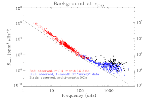
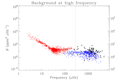
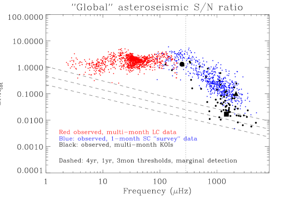
Figure 1: Top left-hand panel: measured background power spectral density, $B_{\rm max}$, at the frequency of maximum oscillation power, $\nu_{\rm max}$, for three cohorts of solar-like oscillators observed by Kepler (see text and annotation for details). The right-hand axis shows the equivalent rms noise per 58.85-sec short-cadence (SC) sample. Top right-hand panel: measured backgrounds at high frequency, which are dominated by shot noise. Middle panel: asteroseismic global signal-to-noise ratios $\rm SNR_{tot}$ for stars in the target cohorts plotted in the top panel. The dashed lines show guideline ratios required for marginal detection of the oscillations assuming datasets of length 3 months (highest lying line), 1 year, and 4 years (lowest lying line). Vertical dotted lines mark the Nyquist frequency for long-cadence observations. Bottom panels: Oscillation spectra of three KOIs, with their $\rm SNR_{tot}$ indicated by the matching symbols in the middle panel.

The top left-hand panel shows the measured background power spectral density, $B_{\rm max}$, at the frequency $\nu_{\rm max}$ where the oscillations present their maximum observed power. The right-hand axis shows the equivalent rms noise per 58.85-sec short-cadence (SC) sample. We show results for all stars in three cohorts of solar-like oscillators observed by Kepler: KASC solar-type targets, KASC red-giant targets, and Kepler Objects of Interest (predominantly solar-type stars, with a few red giants). More details on the cohorts are given below. The plotted $B_{\rm max}$ have contributions from shot and instrumental noise, as well as intrinsic stellar noise. The right-hand panel shows the measured backgrounds at high frequency. These backgrounds are dominated by shot noise, and so reflect the native precision of the Kepler photometry. In sum, both plots show background noise levels that allowed detailed asteroseismic studies to be performed using the nominal-Mission data.

The middle panel of Fig. 1 shows “global” asteroseismic signal-to-noise ratios, $\rm SNR_{tot}$, for stars in the target cohorts plotted in the top panel. We calculated these ratios by dividing the total power observed in the oscillations spectrum of each star by the integrated background power across the frequency range occupied by the observed oscillations (see Chaplin et al. 2011b). It is important to note that values of $\rm SNR_{tot}$ can be much less than unity and still yield a prominent detection of the oscillations. The dashed lines show guideline ratios required for marginal detection of the oscillations assuming datasets of length 3 months (highest lying line), 1 year, and 4 years (lowest lying line). These thresholds are based on a false-alarm test (again, see Chaplin et al. 2011b), which depends in part on the number of frequency bins occupied by the oscillation spectrum. The spectra are much narrower at low frequencies, and this is what drives the higher thresholds needed there for detection (the requirements are probably unduly pessimistic for the very lowest frequencies). Finally, the bottom panels show the oscillation spectra of three Kepler Objects of Interest (see below), with their $\rm SNR_{tot}$ indicated by the matching symbols in the middle panel.

Details on the three cohorts are as follows. The first cohort comprises more than 600 solar-type stars with detected oscillations, and results on these stars are plotted in blue. These stars were selected by the Kepler Asteroseismic Science Consortium (KASC) to be observed for one month each during an asteroseismic survey conducted during the first 10 months of science operations. The 58.85-sec SC data were needed to detect oscillations in these cool main-sequence and subgiant stars, since the dominant oscillations have periods of the order of minutes. These short periods are not accessible to the 29.4-minute long-cadence (LC) data, for which the Nyquist frequency is $\simeq 283\,\rm\mu Hz$ (marked here by the vertical dotted line in both panels). These SC targets all have Kepler apparent magnitudes brighter than $K\rm p\simeq 12$, with one quarter brighter than $K\rm p\simeq 10$. Around 150 of the stars were subsequently observed in SC for at least one observing quarter or longer, with around 60 targets having continuous multi-year data from Q5 onwards. The second cohort comprises targets in black, which are asteroseismic Kepler Objects of Interest (KOIs), i.e., candidate, validated or confirmed exoplanet host stars showing detected solar-like oscillations. All but a handful of the targets are solar-type stars that were observed in SC. Many were put on long-term SC observations because of their potential to yield asteroseismic data for host-star characterization (based on asteroseismic detection predictions made using the procedures described by Chaplin et al. 2011b). Most of these datasets are therefore at least a year in length. This target cohort also extends to fainter apparent magnitudes than the KASC SC cohort, i.e., some stars were observed in the expectation that they would yield only a marginal, but nevertheless extremely useful, asteroseismic detection. The third cohort comprises stars plotted in red, which are KASC red-giant targets. Red giants pulsate at longer periods than solar-type stars, and their oscillations are therefore accessible in the LC data. We note that in addition to these KASC targets, solar-like oscillations have to date also been detected in around another 14,000 Kepler targets. The KASC targets have apparent magnitudes $K\rm p\simeq 11$ to 12; the other cohorts extend down to $K\rm p\simeq 14$.

In all but the faintest solar-type stars it is the contribution from granulation which dominates the background $B_{\rm max}$. The dot-dashed line in the top left-hand panel of Fig. 1 is a simple model of the background contribution due to granulation (see Chaplin et al. 2011b; Mosser et al. 2012c). The spread in the backgrounds for the solar-type stars reflects the significant contribution from photon shot noise in many of these targets (in particular for the faintest KOIs). The middle panel of Fig. 1 also shows the low $\rm SNR_{tot}$ shown by some of the KOIs (which required long datasets to yield an asteroseismic detection).

Going to lower frequencies, the background contribution due to stellar granulation increases in strength, and the distribution of plotted points narrows in power. The $\rm SNR_{tot}$ increase toward lower frequencies, through the subgiant phase. This is due to the diminishing relative contribution to the background from shot noise, whilst at the same time the power due to oscillations and granulation increases. Indeed, the eventual flattening of the ratios can be understood in terms of energy equipartition (the near-surface convection excites the oscillations, so power in the granulation and oscillations might be expected to change in the same way). The increased density of points at around $\simeq 30\,\rm\mu Hz$ is due to low-mass stars in the relatively long-lived He-core-burning (red-clump) phase.

3 Photometric simulations

Our simulations of 2-wheel Kepler photometry were made using the model developed by De Ridder, Kjeldsen & Arentoft (2006). It simulates space-based photometric lightcurves given by CCD images, with all significant instrumental effects included. Full details of the simulations are given by Kjeldsen et al. (2013a, b) [note that tested pointing scenarios have been updated since these documents were published]. Here, we summarize the main points.

Drift is the main source of instrumental noise at low frequencies, and this is corrected almost entirely by the reaction wheels. The high-frequency attitude noise is a result of spacecraft motion that cannot be removed by use of the guiding sensors or corrected by use of the reaction wheels. In the simulations we therefore kept the high-frequency noise component unchanged (as per the specifications in Fig. 18 of the Kepler Instrument Handbook), but increased the low-frequency noise to simulate the degraded performance of the Kepler attitude in 2-wheel mode.

An important part of the simulation is the CCD sensitivity variation. There are three major components that are used to describe the relevant sensitivity variations:

• Global pixel-to-pixel (inter-pixel) variations: In the simulations we assumed a 5 % peak-to-peak sensitivity variability. This variability was chosen to be consistent with the 1 % standard deviation in response non-uniformity given in the Kepler Instrument Handbook. We assumed that 80 % of the global pixel-to-pixel variation can be removed via flat fielding, as discussed in the Section 4.14 of the Kepler Instrument Handbook.

• Random intra-pixel variations: We adopted a 25 % peak-to-peak variability within each pixel (on a scale corresponding to 1 % of the pixel area).

• Sensitivity drops due to pixel-channel (i.e., intra-pixel drops due to the gate structure of the CCD chip): We used 10 % drop along 10 % of a pixel, in both orthogonal directions on the CCD.

Having specified drift and jitter due to the degraded attitude control—details of which are given in Section 4—we used a typical Kepler point-spread-function to create artificial CCD images, which could then be analyzed. The photometric analysis was performed using three different apertures (defined in the software). We also measured the position of the point-spread-function on the simulated CCD, which could then be compared to the attitude inputs. The simulated lightcurves we produced contained only the predicted photometric variability due to the pointing noise, which could then be compared to the performance metrics for the nominal-Mission data presented in Fig. 1.

4 Simulation results and comments

In the following we use the spacecraft coordinate system described in the Call for White Papers document. The two functioning reaction wheels will be used to control the Y and Z axes, while leaving the X axis (which points in the direction of the boresight) to drift.

4.1 Observations in the ecliptic

We began by simulating observations which approximate an extremely favorable observing configuration, that of observing targets in the ecliptic with the boresight pointing approximately in the direction (or anti-direction) of the velocity vector of Kepler in its orbit. This configuration has the Sun in the “balancing” X-Y plane, which minimizes torques due to solar radiation pressure (which would induce roll about the X axis).

We assumed a non-linear (accelerating) roll totalling 120 arcsec per day (to match approximately the predictions in the document Explanatory Appendix to the Call for White Papers), with short-term rms jitter of 1 arcsec. This gives a few pixels of drift for targets lying on the edge of the field of view (the case we tested), less for pixels lying close to the centre. Momentum management demands regular desaturation of the two functioning wheels, and here we assumed a daily cycle, whereby the pointing of the spacecraft was reset every day. Moreover, we also considered the most favorable reset scenario, in which targets were assumed to go back each day to follow identical pixel trails on the CCD array. Here, at each simulated daily reset we simply moved targets back to the same pixels on our simulated array (but with the jitter imposed independently on each repeat). It should be borne in mind that it may be difficult in practice to achieve this level of re-pointing. Offsets at the first pointing would also propagate to give elevated levels of drift, over and above those assumed above. However, as we shall see below, the raw results from this assumed scenario are sufficient to allow us to reach conclusions on asteroseismic detectability levels in less favorable cases; and, very importantly, they also allow us to comment on prospects for continuation of observations in the Kepler field-of-view (of which more below in Section 4.2).

Finally—and of crucial importance for our main conclusions—we also applied a post-hoc correction to the photometry by using the repeated daily tracking across the same pixels to produce a model of the local inter- and intra-pixel variability. Details of this procedure may be found in Kjeldsen et al. (2013a). Assuming that the detector sensitivity is stable in time, when a star moves back to the same position on the CCD several times one may use the measured photometry and the measured stellar positions on the CCD to generate a model which separates the intra- and inter-pixel sensitivity from other variations in time, to in principle leave the intrinsic noise and the stellar variability. The quality of the model depends on several factors, e.g., how often the star is moved back to the same position, and the drift rate during exposures. SC data will offer better possibilities for this correction than LC data. It is important to stress that our results from applying this procedure rest on the assumed best-case re-pointing. They should therefore be regarded as an approximate guide to the “limiting” ideal case for the photometry. We have also applied the test to simulated SC, not LC, data.

Fig. 2 shows results from the simulations. The thick black line in the top left-hand panel shows the power spectral density given by a simulated 30-day lightcurve of raw SC pointing noise. The spectrum has been smoothed for clarity with a 10-$\rm\mu Hz$ boxcar filter. The thick line in the right-hand panel shows the smoothed pointing-noise spectrum after applying a post-hoc model to the raw data to correct for variations in CCD sensitivity. We also plot for comparison (in gray) the $B_{\rm max}$ values for the nominal-Mission data, which were plotted in the top left-hand panel of Fig. 1. The scales on the right-hand axes again show the equivalent rms noise per SC sample.

We may estimate the impact on the asteroseismic signal-to-noise ratios $\rm SNR_{tot}$ by adding the frequency-dependent pointing noise power to the nominal-Mission $B_{\rm max}$. The bottom left-hand panel shows the re-calculated ratios with the effects of the raw pointing noise included; whilst the right-hand panel shows the ratios after the post-hoc CCD corrections have been applied. Corrected ratios are plotted in color; while the nominal-Mission ratios from Fig. 1 are shown in gray for comparison.

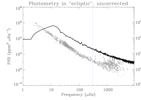
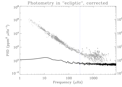
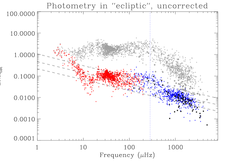
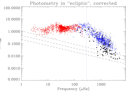
Figure 2: Top left-panel: Power spectral density given by a simulated 30-day lightcurve of raw pointing noise. Top right-hand panel: Power spectral density after applying a post-hoc model to the raw data to correct for variations in CCD sensitivity. Both panels show in gray the $B_{\rm max}$ values for the nominal-Mission data (see top left-hand panel of Fig. 1). The right-hand axes show the equivalent rms noise per SC sample. Bottom left-hand panel: re-calculated $\rm SNR_{tot}$ with the effects of the raw pointing noise included. Gray points show ratios from nominal-Mission data. Right-hand panel: re-calculated ratios after post-hoc CCD corrections have been applied.

The rms scatter in the time domain of the raw pointing-noise is about $2500\,\rm ppm$ per SC sample. The pointing noise has a strong frequency dependence, and is higher than the nominal-Mission backgrounds at essentially all frequencies. Not surprisingly, there is also significant power at harmonics of 1 day (suppressed visually here by the smoothing applied for the plot). It is worth noting that since the simulated lightcurve was only 30 days long—and is but one realization for a given track across the simulated CCD—there would probably be significant variability in the pointing-noise power at very low frequencies. Predictions there should be treated with caution.

The strongly degraded $\rm SNR_{tot}$ ratios in the bottom left-hand panel show that the asteroseismic quality would be reduced significantly, leading to null detections for many targets and perhaps only marginal detections for others. Further tests indicated that the simulated levels of noise—and hence the predicted outcomes for asteroseismology—appear to depend critically on the assumed levels of short-term jitter, in particular for the higher frequencies. The results appear to be less sensitive to changes in the rate of drift (assuming manageable rates).

The situation becomes rather more encouraging if one assumes that a post-hoc model could successfully be applied to real 2-wheel Kepler data (right-hand panels of Fig. 2). The rms scatter of the corrected lightcurve—around $50\,\rm ppm$ per SC sample—is significantly lower than that of the raw lightcurve. The corrected pointing-noise background lies below the nominal-Mission backgrounds for all but a few of the very brightest SC targets (where the nominal-Mission precision was as low as a few-tens of ppm). The corrected $\rm SNR_{tot}$ ratios in the bottom right-hand panel are little changed from the nominal-Mission values, indicating that asteroseismology of solar-like oscillators would in principle be possible for targets in the ecliptic. It is important to remember that this outcome would rest on the assumption that re-pointing is accurate at the individual pixel level (i.e., probably demanding a $1\sigma$ precision of $\leq 1\,\rm arcsec$).

Observations in the ecliptic would open exciting possibilities for new targets, e.g., with reference to Section 1.2, the clusters M67 and M44; and new ensembles of solar-type stars and red-giant field stars not previously observed for asteroseismology, which would provide data for stellar evolution and interiors physics studies, and fundamental stellar properties for stellar population studies in new fields, and exoplanet host-star characterization (assuming continuation of exoplanet searches). Studies of the clusters could enable science that was not possible in the nominal Mission (and which would be unique): we would potentially be able for the first time to exploit data on solar-like oscillations in main-sequence cluster stars. Studies of surface rotation and activity, from variability in the lightcurves, would probably also be viable on rapidly rotating solar-type stars. Tests on longer timescales would be needed to judge prospects for more slowly rotating solar-type stars and red giants.

Targets would not be observable all year round. One potential observing strategy would have Kepler follow targets for 3 months (with Kepler pointed exactly along the velocity vector, say, half-way through the period); then re-point to another field for 3 months; and then go back to the original field (with Kepler pointed against the velocity); and so on. This would provide up to 6 months of data on some stars every year. Demands on pointing would vary throughout each 3-month period. It would be highly desirable to have pixel tracks of the same length, which would require a varying cadence for the desaturation events. Again, our results rest on the assumption of consistently achievable, very accurate re-pointing. The most attractive strategy for asteroseismology would then arguably be one in which Kepler came back to the same targets every year, allowing the accumulation of up to 1 or 2 years of data after 2 or 4 years of 2-wheel science operations. Other choices would also of course be possible, depending on the selection of specific targets in the ecliptic. Long, 3-month gaps in coverage would not pose a significant obstacle to the analysis of main-sequence stars. The lifetimes of modes observed in these stars are typically much shorter, of the order of days. The lifetimes of mixed modes and gravity dominated modes observed in more evolved stars are somewhat longer; however, the effects of long gaps can in principle be modelled and accounted for. There would also be repeated desaturation gaps, but they should be short and not a significant issue for the analysis.

4.2 Observations in the Kepler field-of-view

Next, we comment on the extremely important scenario of continuing observations in the Kepler field-of-view. This scenario has the added complication that the Sun drifts relative to the X-Y plane of the spacecraft by 1 degree per day. The spacecraft must therefore be rolled on a regular basis to maintain the Sun in the balancing X-Y plane. Frequent rolls (probably daily) would be required to keep drift rates manageable, and to ensure they would not become problematic for target aperture allocations. Targets will not return to the same pixel tracks on the CCD array and it would therefore not be possible to use the post-hoc procedure to model and then correct the raw photometry.

To simulate the impact of an assumed daily roll, we simply reset targets each day in our simulation to a different part of the simulated array. It should also be noted that our simulations did not include complications that would arise from changing stray-light levels (from the daily rolls). These revised simulations gave results that were similar to the uncorrected ecliptic case discussed above (again indicating the importance of jitter, which was the same in both sets of simulations, versus the impact of manageable drift, which was not). Bearing in mind the simulation results in the left-hand panels of Fig. 2, the prospects for continuing asteroseismology of solar-like oscillators in the Kepler field do not look good (unless the pointing noise specifications we have tested turn out to be unduly pessimistic).

5 Concluding remarks

We have performed our own simulations of the pointing noise expected for 2-wheel Kepler observations of targets in the Kepler field-of-view, and in the ecliptic. Having results on the frequency dependence of the noise is critical to judging the potential to continue asteroseismic studies of solar-like oscillators. We find that while elevated levels of noise would impact significantly on our ability to continue such studies in the Kepler field, the situation is potentially much more optimistic for observations in the ecliptic. However, that optimism rests on the important assumption that pointing resets during regular desaturations of the two functioning wheels would be accurate at the $\leq 1\,\rm arcsec$ level. This would ensure that when targeting a given field, stars would follow the same pixel tracks on the CCD after each desaturation and reset, making it possible to apply a post-hoc analysis to recover most of the photometric precision lost by the inferior pointing. Our simulations indicate that Kepler would then be able to provide good data for asteroseismology. Assuming good pointing performance, it would probably be possible to use the existing readout software with slightly increased aperture masks.

A crucial part of our paper is the set of “baseline” asteroseismic performance metrics, which come from analysis results on the nominal-Mission data. Once full simulation results on the actual expected (frequency-dependent) performance are available—courtesy of the Kepler Project and Ball Aerospace (the spacecraft manufacturer)—it will be possible to use the metrics presented in this paper (and accompanying data that we did not have the space to include) to make a definitive assessment of whether continuation of asteroseismic studies of solar-like oscillators is feasible. We will also be able to test observations in other fields (including pointing just off the ecliptic).

References

Barclay, T., et al., 2013, Nature, 494, 452

Basu, S., et al., 2010, ApJ, 729, L10

Beck, P. G., et al., 2012, Nature, 481, 55

Bedding, T. R., et al., 2011, Nature, 471, 608

Carter, J. A., et al., 2012, Science, 337, 556

Chaplin, W. J., et al., 2011a, Science, 332, 213

Chaplin, W. J., et al., 2011b, ApJ, 732, 54

Chaplin, W. J., et al., 2013, ApJ, 766, 101

Corsaro, E., et al., 2012, ApJ, 757, 190

Deheuvels, S., et al., 2012, ApJ, 756, 19

De Ridder, J., et al., 2006, MNRAS, 365, 595

García, R. A., et al., 2010, Science, 329, 1032

Gilliland, R. L., et al., 2010, PASP, 122, 131

Gilliland, R. L., et al., 2013, ApJ, 766, 40

Hekker, S., et al., 2011, MNRAS, 414, 2594

Huber, D., et al., 2011, ApJ, 743, 143

Huber, D., et al., 2013, ApJ, 767, 127

Kallinger, T., et al., 2012, A&A, 522, 1

Karoff, C., et al., 2009, MNRAS, 399, 914

Kjeldsen, H., et al., 2013a, KASC document, DASC/KASOC/0043(2)

(http://astro.phys.au.dk/~hans/Call_for_White_Paper/DASC_KASOC_0043_2.pdf)

Kjeldsen, H., et al., 2013b, KASC document, DASC/KASOC/0044(1)

(http://astro.phys.au.dk/~hans/Call_for_White_Paper/DASC_KASOC_0044_1.pdf)

Mazumdar, A., et al., 2013, ApJ, submitted

Metcalfe, T. S., et al., 2010, ApJ, 723, 1583

Metcalfe, T. S., et al., 2012, ApJ, 748, L10

Miglio, A., 2012, ASSP (ISBN 978-3-642-18417-8), p. 11

Miglio, A., et al., 2012, MNRAS, 419, 2077

Mosser, B., et al., 2012a, A&A, 540, 143

Mosser, B., et al., 2012b, A&A, 548, 10

Mosser, B., et al., 2012c, A&A, 537, 30

Silva Aguirre, V., et al., 2013, ApJ, 769, 141

Stello, D., et al., 2010, ApJ, 713, L182

Stello, D., et al., 2013, ApJ, 765, L41

Kepler Instrument Handbook, KSCI-19033, 15 July 2009, NASA Ames Research Center

(http://keplerscience.arc.nasa.gov/calibration/KSCI-19033-001.pdf)

Call for White Papers: Soliciting Community Input for Alternative Science Investigations for the Kepler Spacecraft

(http://keplergo.arc.nasa.gov/docs/Kepler-2wheels-call-1.pdf)

Explanatory Appendix to the Kepler Project call for White Papers: Kepler 2-Wheel Pointing Control

(http://keplergo.arc.nasa.gov/docs/Kepler-2-Wheel-pointing-performance.pdf)