Denoising Using Projection Onto Convex Sets (POCS) Based Framework

Abstract

Two new optimization techniques based on projections onto convex space (POCS) framework for solving convex optimization problems are presented. The dimension of the minimization problem is lifted by one and sets corresponding to the cost function are defined. If the cost function is a convex function in $R^{N}$ the corresponding set is also a convex set in $R^{N+1}$. The iterative optimization approach starts with an arbitrary initial estimate in $R^{N+1}$ and an orthogonal projection is performed onto one of the sets in a sequential manner at each step of the optimization problem. The method provides globally optimal solutions in total-variation (TV), filtered variation (FV), $\ell_{1}$, and entropic cost functions. A new denoising algorithm using the TV framework is developed. The new algorithm does not require any of the regularization parameter adjustment. Simulation examples are presented.

I Introduction

In many inverse signal and image processing problems and compressing sensing problems an optimization problem is solved to find a solution to the following problem:

$$\underset{\mathbf{w}\in\text{C}}{\text{min}}f(\mathbf{w}),$$ (1)

where $\mathbb{C}$ is a set in $\mathbb{R}^{N}$ and $f(\mathbf{w})$ is the cost function. Some commonly used cost functions are based on $\ell_{1}$, $l_{2}$, total-variation (TV), filtered variation, and entropic functions [1, 2, 3, 4, 5]. Bregman developed iterative methods based on the so-called Bregman distance to solve convex optimization problems which arise in signal and image processing [6]. In Bregman’s approach, it is necessary to perform a D-projection (or Bregman projection) at each step of the algorithm and it may not be easy to compute the Bregman distance in general [7, 8, 5].

In this article Bregman’s older projections onto convex sets (POCS) framework [9, 10] is used to solve convex and some non-convex optimization problems instead of the Bregman distance approach. Bregman’s POCS method has also been widely used for finding a common point of convex sets in many inverse signal and image processing problems[10, 11, 12, 13, 14, 15, 16, 17, 18, 19, 20, 21, 22, 23, 24, 25, 26, 27, 28, 29, 30, 31, 32, 33]. In the ordinary POCS approach the goal is simply to find a vector which is in the intersection of convex sets. In each step of the iterative algorithm an orthogonal projection is performed onto one of the convex sets. Bregman showed that successive orthogonal projections converge to a vector which is in the intersection of all the convex sets. If the sets do not intersect iterates oscillate between members of the sets [34, 35, 36]. Since there is no need to compute the Bregman distance in standard POCS, it found applications in many practical problems.

In our approach the dimension of the minimization problem is lifted by one and sets corresponding to the cost function are defined. This approach is graphically illustrated in Fig. 1. If the cost function is a convex function in $R^{N}$ the corresponding set is also a convex set in $R^{N+1}$. As a result the convex minimization problem is reduced to finding a specific member (the optimal solution) of the set corresponding to the cost function. As in ordinary POCS approach the new iterative optimization method starts with an arbitrary initial estimate in $R^{N+1}$ and an orthogonal projection is performed onto one of the sets. After this vector is calculated it is projected onto the other set. This process is continued in a sequential manner at each step of the optimization problem. The method provides globally optimal solutions in total-variation, filtered variation, $\ell_{1}$, and entropic function based cost functions because they are convex cost functions.

The article is organized as follows. In Section II, the convex minimization method based on the POCS approach is introduced. In Section III, a new denoising method based on the convex minimization approach introduced in Section II, is presented.This new approach uses supporting hyperplanes of the TV function and it does not require a regularization parameter as in other TV based methods. Since it is very easy to perform an orthogonal projection onto a hyperplane this method is computationally implementable for many cost functions without solving any nonlinear equations. In Section IV, we present the simulation results and some denoising examples.

II Convex Minimization

Let us first consider a convex minimization problem

$$\underset{\mathbf{w}\in\mathbb{R}^{N}}{\text{min}}f(\mathbf{w}),$$ (2)

where $f:\mathbb{R}^{N}\rightarrow\mathbb{R}$ is a convex function. We increase the dimension by one to define the following sets in $\mathbb{R}^{N+1}$ corresponding to the cost function $f(\mathbf{w})$ as follows:

$$\text{C}_{f}=\{\underline{\mathbf{w}}=[\mathbf{w}^{T}~{}y]^{T}:\mathrm{~{}}y\geq f(\mathbf{w})\},$$ (3)

which is the set of $N+1$ dimensional vectors whose $(N+1)^{st}$ component $y$ is greater than $f(\mathbf{w})$. This set $C_{f}$ is called the epigraph of $f$. We use bold face letters for $N$ dimensional vectors and underlined bold face letters for $N+1$ dimensional vectors, respectively.

The second set that is related with the cost function $f(\mathbf{w})$ is the level set:

$$\text{C}_{s}=\{\underline{\mathbf{w}}=[\mathbf{w}^{T}~{}y]^{T}:~{}y\leq\alpha,~{}\underline{\mathbf{w}}\in\mathbb{R}^{N+1}\},$$ (4)

where $\alpha$ is a real number. Here it is assumed that $f(\mathbf{w})\geq\alpha$ for all $f(\mathbf{w})\in\mathbb{R}$ such that the sets $C_{f}$ and $C_{s}$ do not intersect. They are both closed and convex sets in $\mathbb{R}^{N+1}$. Sets $C_{f}$ and $C_{s}$ are graphically illustrated in Fig. 1 in which $\alpha=0.$

Figure 1: Two convex sets $C_{f}$ and $C_{s}$ corresponding to the cost function $f$. We sequentially project an initial vector $\underline{\mathbf{w}}_{0}$ onto $C_{s}$ and C$C_{f}$ to find the global minimum which is located at $\mathbf{w}^{*}$.

The POCS based minimization algorithm starts with an arbitrary $\underline{\mathbf{w}}_{0}=[\mathbf{w}_{0}^{T}~{}y_{0}]^{T}\in\mathbb{R}^{N+1}$. We project $\underline{\mathbf{w}}_{0}$ onto the set $C_{s}$ to obtain the first iterate $\underline{\mathbf{w}}_{1}$ which will be,

$$\underline{\mathbf{w}}_{1}=[\mathbf{w}_{0}^{T}~{}0]^{T},$$ (5)

where $\alpha=0$ is assumed as in Fig. 1. Then we project $\underline{\mathbf{w}}_{1}$ onto the set $C_{f}$. The new iterate $\underline{\mathbf{w}}_{2}$ is determined by minimizing the distance between $\underline{\mathbf{w}}_{1}$ and $C_{f}$, i.e.,

$$\underline{\mathbf{w}}_{2}=\text{arg}\underset{\underline{\mathbf{w}}\in\text{C}_{\mathrm{s}}}{\text{min}}\|\underline{\mathbf{w}}_{1}-\underline{\mathbf{w}}\|.$$ (6)

Equation 6 is the ordinary orthogonal projection operation onto the set $\mathrm{C_{f}}\in\mathbb{R}^{N+1}$. To solve the problem in Eq. 6 we do not need to compute the Bregman’s so-called D-projection. After finding $\underline{\mathbf{w}}_{2}$, we perform the next projection onto the set $C_{s}$ and obtain $\underline{\mathbf{w}}_{3}$ etc. Eventually iterates oscillate between two nearest vectors of the two sets $C_{s}$ and $C_{f}$. As a result we obtain

$$\underset{n\rightarrow\infty}{\text{lim}}\underline{\mathbf{w}}_{2n}=[\mathbf{w}^{*}~{}f(\mathbf{w}^{*})]^{T},$$ (7)

where $\mathbf{w}^{*}$ is the N dimensional vector minimizing $f(\mathbf{w})$. The proof of Eq. 7 follows from Bregman’s POCS theorem [9, 34]. It was generalized to non-intersection case by Gubin et. al [34, 12],[35]. Since the two closed and convex sets $C_{s}$ and $C_{f}$ are closest to each other at the optimal solution case, iterations oscillate between the vectors $[\mathbf{w}^{*}~{}f(\mathbf{w}^{*})]^{T}$ and $[\mathbf{w}^{*}~{}0]^{T}$ in $R^{N+1}$ as $n$ tends to infinity. It is possible to increase the speed of convergence by non-orthogonal projections [24].

If the cost function $f$ is not convex and have more than one local minimum then the corresponding set $C_{f}$ is not convex in $R^{N+1}$. In this case iterates may converge to one of the local minima.

III Denoising Using POCS

In this section, we present a new method of denoising, based on TV and FV. Let the noisy signal be y, and the original signal or image be $\textbf{w}_{0}$. Suppose that the observation model is the additive noise model:

$$\textbf{y}=\textbf{w}_{0}+\textbf{v},$$ (8)

where v is the additional noise. In this approach we solve the following problem for denoising:

$$\underline{\mathbf{w}}^{\star}=\text{arg}\underset{\underline{\mathbf{w}}\in\text{C}_{\mathrm{f}}}{\text{min}}\|\underline{\mathbf{y}}-\underline{\mathbf{w}}\|^{2},$$ (9)

where, $\underline{\mathbf{y}}$ = [$y^{T}$ 0] and $C_{f}$ is the epigraph set of TV or FV in $R^{N+1}$. The minimization problem is essentially the orthogonal projection onto the set $C_{f}$. This means that we select the nearest vector $\underline{\mathbf{w}}^{\star}$ on the set $C_{f}$ to y. This is graphically illustrated in Fig. 2.

Figure 2: Graphical representation of the minimization of (9). y is projected onto the set $C_{f}$. TV(w) is zero for $\textbf{w}=[0,0,...,0]^{T}$ or when it is a constant vector.

Figure 3: Graphical representation of the minimization of (9), using projection onto the supporting hyperplanes of $C_{f}$.

In current TV based denoising methods [37, 38] the following cost function is used:

$${{\text{min}}\|\underline{\mathbf{y}}-\underline{\mathbf{w}}\|}^{2}_{2}+\lambda\text{TV}(\textbf{w}).$$ (10)

The solution of this problem can be obtained using the method that we discussed in Section II. One problem with this approach is the estimation of the regularization parameter $\lambda$. One has to determine the $\lambda$ in an ad hoc manner or by visual inspection. On the other hand we do not require any parameter adjustment in (9).

The denoising solution in (9) can be found by performing successive orthogonal projection onto supporting hyperplanes of the epigraph set $C_{f}$. In the first step we calculated TV($\mathbf{y}$). We also calculate the surface normal at $\underline{\mathbf{y}}$ = [$\mathbf{y}^{T}$  TV($\mathbf{y}$)] in $R^{N+1}$ and determine the equation of the supporting hyperplane at [$\mathbf{y}^{T}$  TV($\mathbf{y}$)]. We project $\underline{\mathbf{y}}$ = [$\mathbf{y}^{T}$  0] onto this hyperplane and obtain $\underline{\mathbf{w}}_{1}$ as our first estimate as shown in Fig. 3. In the second step we project $\underline{\mathbf{w}}_{1}$ onto the set $C_{s}$ by simply making its last component zero. We calculate the TV of this vector and the surface normal, and the supporting hyperplane as in the previous step. We project $\underline{\mathbf{y}}$ onto the new supporting hyperplane, etc.

The sequence of iterations obtained in this manner converges to a vector in the intersection of $C_{s}$ and $C_{f}$. In this problem the sets $C_{s}$ and $C_{f}$ intersect because $TV(\textbf{w})=0$ for $\textbf{w}=[0,0,...,0]^{T}$ or for a constant vector. However, we do not want to find a trivial constant vector in the intersection of $C_{s}$ and $C_{f}$. We calculate the distance between $\underline{\mathbf{y}}$ and $\underline{\mathbf{w}}_{i}$ at each step of the iterative algorithm described in the previous paragraph. This distance ${\|\underline{\mathbf{y}}-\underline{\mathbf{w}}\|}^{2}_{2}$ initially decreases and starts increasing as $i$ increases. Once we detect the increase we perform some refinement projections to obtain the solution of the denoising problem. A typical convergence graph is shown in Fig. 4 for the “note” image.

Figure 4: Orthogonal distance from y to the epigraph of TV in each iteration.

Simulation exapmles are presented in the next section.

IV Simulation Results

Consider the “Note” image shown in Fig. 5. This is corrupted by a zero mean Gaussian noise with $\lambda=45$ in Fig. 6. The image is restored using our method and Chombolle’s algorithm [37] and the denoised images are shown in Fig. 7 and 8, respectively. The $\lambda$ parameter in (10) is manually adjusted to get the best possible results. Our algorithm not only produce a higher SNR, but also a visually better looking image. Solution results for other SNR levels are presented in Table I. We also corrupted this image with $\epsilon$-contaminated Gaussian noise (“salt-and-pepper noise”). Denoising results are summarized in Table II.

In Table III, denoising results for 10 other images with different noise levels are presented. In almost all cases our method produces higher SNR results than the denoising results obtained using [37].

TABLE I: Comparison of The Results For Denoising Algorithms With Gaussian Noise For Note Image

Noise std	Input SNR	POCS	Chambolle
5	21.12	30.63	29.48
10	15.12	25.93	24.20
15	11.56	22.91	21.05
20	9.06	20.93	18.90
25	7.14	19.27	17.17
30	5.59	17.89	15.78
35	4.21	16.68	14.69
40	3.07	15.90	13.70
45	2.05	15.08	12.78
50	1.12	14.25	12.25

TABLE II: Comparison of The Results For Denoising Algorithms for $\epsilon$-Contamination Noise For Note Image

$\epsilon$	$\sigma_{1}$	$\sigma_{2}$	Input SNR	POCS	Chambolle
0.9	5	30	14.64	23.44	20.56
0.9	5	40	12.55	21.39	17.60
0.9	5	50	10.75	19.49	15.54
0.9	5	60	9.29	17.61	13.82
0.9	5	70	7.98	16.01	12.57
0.9	5	80	6.89	14.54	11.37
0.9	10	30	12.56	22.88	19.74
0.9	10	40	11.13	21.00	15.30
0.9	10	50	9.85	19.35	12.47
0.9	10	60	8.58	17.87	10.42
0.9	10	70	7.52	16.38	8.76
0.9	10	80	6.46	15.05	7.45
0.95	5	30	16.75	24.52	23.18
0.95	5	40	14.98	22.59	20.44
0.95	5	50	13.41	20.54	18.45
0.95	5	60	12.10	18.72	16.80
0.95	5	70	10.80	17.13	15.34
0.95	5	80	9.76	15.63	14.11
0.95	10	30	13.68	23.79	20.43
0.95	10	40	12.66	22.09	15.35
0.95	10	50	11.71	20.65	12.28
0.95	10	60	10.72	19.10	10.22
0.95	10	70	9.82	17.59	8.66
0.95	10	80	8.92	16.12	7.34

Figure 5: Original “Note” image.

Figure 6: “Note” image corrupted with Gaussian noise with $\lambda=45$.

Figure 7: Denoised image “Note” image, using [1 -1] filter; SNR = 15.08.

Figure 8: Denoised image “Note” image, using Chambolle’s algorithm; SNR = 12.78.

TABLE III: Comparison of The Results For Denoising Algorithms With Gaussian Noise For Different Images With std = 30, 50

Images	Noise std	Input SNR	POCS	Chambolle
House	30	13.85	27.43	27.13
House	50	9.45	24.20	24.36
Lena	30	12.95	23.63	23.54
Lena	50	8.50	21.46	21.37
Mandrill	30	13.04	19.98	19.64
Mandrill	50	8.61	17.94	17.92
Living room	30	12.65	21.21	20.88
Living room	50	8.20	19.25	19.05
Lake	30	13.44	22.19	21.86
Lake	50	8.97	20.03	19.90
Jet plane	30	15.57	26.28	25.91
Jet plane	50	11.33	23.91	23.54
Peppers	30	12.65	23.57	23.59
Peppers	50	8.20	21.48	21.36
Pirate	30	12.13	21.39	21.30
Pirate	50	7.71	19.37	19.43
Cameraman	30	12.97	24.13	23.67
Cameraman	50	8.55	21.55	21.22
Flower	30	11.84	21.97	20.89
Flower	50	7.42	19.00	18.88
Average	30	13.11	23.18	22.84
Average	50	8.69	20.82	20.70

V Conclusion

A new denoising method based on the epigraph of the TV function is developed. The solution is obtained using POCS. The new algorithm does not need the optimization of the regularization parameter.

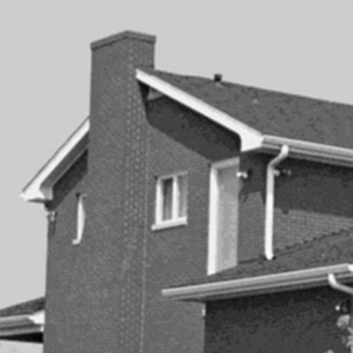
(a) House

(b) Jet plane

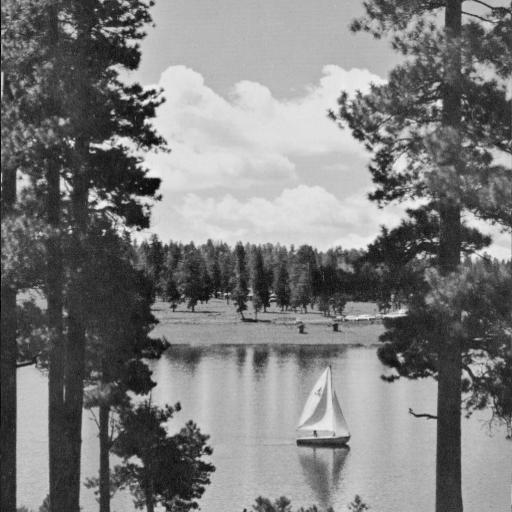
(c) Lake

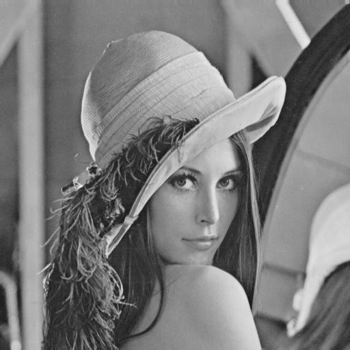
(d) Lena

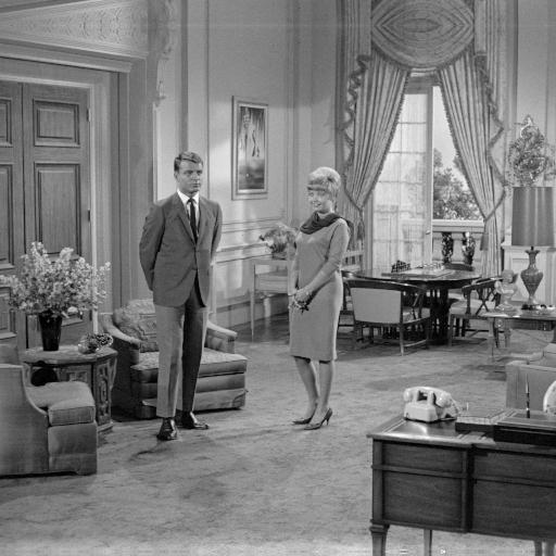
(e) Living room

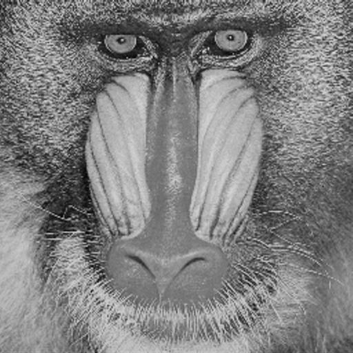
(f) Mandrill

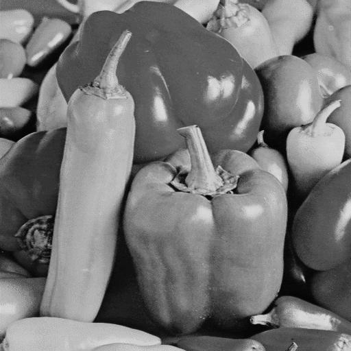
(g) Peppers

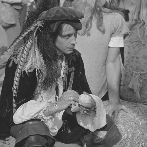
(h) Pirate

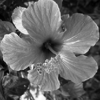
(i) Flower

(j) Cameraman

Figure 9: Sample images used in our experiments (a) House, (b) Jet plane, (c) Lake, (d) Lena, (e) Living room, (f) Mandrill, (g) Peppers, (h) Pirate.

References

- [1] L. I. Rudin, S. Osher, and E. Fatemi, “Nonlinear total variation based noise removal algorithms,” Physica D: Nonlinear Phenomena, vol. 60, no. 1–4, pp. 259 – 268, 1992.
- [2] R. Baraniuk, “Compressive sensing [lecture notes],” Signal Processing Magazine, IEEE, vol. 24, no. 4, pp. 118–121, 2007.
- [3] E. Candes and M. Wakin, “An introduction to compressive sampling,” Signal Processing Magazine, IEEE, vol. 25, no. 2, pp. 21–30, 2008.
- [4] K. Kose, V. Cevher, and A. Cetin, “Filtered variation method for denoising and sparse signal processing,” Acoustics, Speech and Signal Processing (ICASSP), 2012 IEEE International Conference on, pp. 3329–3332, 2012.
- [5] O. Günay, K. Köse, B. U. Töreyin, and A. E. Çetin, “Entropy-functional-based online adaptive decision fusion framework with application to wildfire detection in video,” IEEE Transactions on Image Processing, vol. 21, no. 5, pp. 2853–2865, May 2012.
- [6] L. Bregman, “The Relaxation Method of Finding the Common Point of Convex Sets and Its Application to the Solution of Problems in Convex Programming,” {USSR} Computational Mathematics and Mathematical Physics, vol. 7, no. 3, pp. 200 – 217, 1967.
- [7] W. Yin, S. Osher, D. Goldfarb, and J. Darbon, “Bregman iterative algorithms for -minimization with applications to compressed sensing,” SIAM Journal on Imaging Sciences, vol. 1, no. 1, pp. 143–168, 2008.
- [8] K. Köse, “Signal and Image Processing Algorithms Using Interval Convex Programming and Sparsity,” Ph.D. dissertation, Bilkent University, 2012.
- [9] L. Bregman, “Finding the common point of convex sets by the method of successive projection.(russian),” {USSR} Dokl. Akad. Nauk SSSR, vol. 7, no. 3, pp. 200 – 217, 1965.
- [10] D. Youla and H. Webb, “Image Restoration by the Method of Convex Projections: Part 1 Num2014;theory,” Medical Imaging, IEEE Transactions on, vol. 1, no. 2, pp. 81–94, 1982.
- [11] G. T. Herman, “Image Reconstruction from Projections,” Real-Time Imaging, vol. 1, no. 1, pp. 3–18, 1995.
- [12] Y. Censor, W. Chen, P. L. Combettes, R. Davidi, and G. Herman, “On the Effectiveness of Projection Methods for Convex Feasibility Problems with Linear Inequality Constraints,” Computational Optimization and Applications, vol. 51, no. 3, pp. 1065–1088, 2012.
- [13] K. Slavakis, S. Theodoridis, and I. Yamada, “Online Kernel-Based Classification Using Adaptive Projection Algorithms,” IEEE Transactions on Signal Processing, vol. 56, pp. 2781–2796, 2008.
- [14] A. Çetin, H. Özaktaş, and H. Ozaktas, “Resolution Enhancement of Low Resolution Wavefields with,” Electronics Letters, vol. 39, no. 25, pp. 1808–1810, 2003.
- [15] A. E. Cetin and R. Ansari, “Signal recovery from wavelet transform maxima,” IEEE Transactions on Signal Processing, pp. 673–676, 1994.
- [16] A. E. Cetin, “Reconstruction of signals from fourier transform samples,” Signal Processing, pp. 129–148, 1989.
- [17] K. Kose and A. E. Cetin, “Low-pass filtering of irregularly sampled signals using a set theoretic framework,” IEEE Signal Processing Magazine, pp. 117–121, 2011.
- [18] Y. Censor and A. Lent, “An Iterative Row-Action Method for Interval Convex Programming,” Journal of Optimization Theory and Applications, vol. 34, no. 3, pp. 321–353, 1981.
- [19] K. Slavakis, S. Theodoridis, and I. Yamada, “Adaptive constrained learning in reproducing kernel hilbert spaces: the robust beamforming case,” IEEE Transactions on Signal Processing, vol. 57, no. 12, pp. 4744–4764, dec 2009.
- [20] K. S. Theodoridis and I. Yamada, “Adaptive learning in a world of projections,” IEEE Signal Processing Magazine, vol. 28, no. 1, pp. 97–123, 2011.
- [21] Y. Censor and A. Lent, “Optimization of logx entropy over linear equality constraints,” SIAM Journal on Control and Optimization, vol. 25, no. 4, pp. 921–933, 1987.
- [22] H. Trussell and M. R. Civanlar, “The Landweber Iteration and Projection Onto Convex Set,” IEEE Transactions on Acoustics, Speech and Signal Processing, vol. 33, no. 6, pp. 1632–1634, 1985.
- [23] P. L. Combettes and J. Pesquet, “Image restoration subject to a total variation constraint,” IEEE Transactions on Image Processing, vol. 13, pp. 1213–1222, 2004.
- [24] P. Combettes, “The foundations of set theoretic estimation,” Proceedings of the IEEE, vol. 81, no. 2, pp. 182 –208, February 1993.
- [25] A. E. Cetin and R. Ansari, “Convolution based framework for signal recovery and applications,” JOSA-A, pp. 673–676, 1988.
- [26] I. Yamada, M. Yukawa, and M. Yamagishi, “Minimizing the moreau envelope of nonsmooth convex functions over the fixed point set of certain quasi-nonexpansive mappings,” in Fixed-Point Algorithms for Inverse Problems in Science and Engineering. Springer, 2011, pp. 345–390.
- [27] Y. Censor and G. T. Herman, “On some optimization techniques in image reconstruction from projections,” Applied Numerical Mathematics, vol. 3, no. 5, pp. 365–391, 1987.
- [28] I. Sezan and H. Stark, “Image restoration by the method of convex projections: Part 2-applications and numerical results,” IEEE Transactions on Medical Imaging, vol. 1, no. 2, pp. 95–101, 1982.
- [29] Y. Censor and S. A. Zenios, “Proximal minimization algorithm withd-functions,” Journal of Optimization Theory and Applications, vol. 73, no. 3, pp. 451–464, 1992.
- [30] A. Lent and H. Tuy, “An Iterative Method for the Extrapolation of Band-Limited Functions,” Journal of Mathematical Analysis and Applications, 83 (2), pp.1981, vol. 83, pp. 554–565, 1981.
- [31] Y. Censor, “Row-action methods for huge and sparse systems and their applications,” SIAM review, vol. 23, no. 4, pp. 444–466, 1981.
- [32] Y. Censor, A. R. De Pierro, and A. N. Iusem, “Optimization of burg’s entropy over linear constraints,” Applied Numerical Mathematics, vol. 7, no. 2, pp. 151–165, 1991.
- [33] M. Rossi, A. M. Haimovich, and Y. C. Eldar, “Conditions for Target Recovery in Spatial Compressive Sensing for MIMO Radar,” 2013.
- [34] L. Gubin, B. Polyak, and E. Raik, “The Method of Projections for Finding the Common Point of Convex Sets,” {USSR} Computational Mathematics and Mathematical Physics, vol. 7, no. 6, pp. 1 – 24, 1967.
- [35] P. L. Combettes, “Algorithmes proximaux pour lés problemes d´optimisation structur les,” 2012.
- [36] A. E. Çetin, O. Gerek, and Y. Yardimci, “Equiripple FIR Filter Design by the FFT Algorithm,” IEEE Signal Processing Magazine, vol. 14, no. 2, pp. 60–64, 1997.
- [37] A. Chambolle, “An algorithm for total variation minimization and applications,” J. Math. Imaging Vis., vol. 20, no. 1-2, pp. 89–97, Jan. 2004.
- [38] P. L. Combettes and J.-C. Pesquet, “Proximal splitting methods in signal processing,” in Fixed-Point Algorithms for Inverse Problems in Science and Engineering, ser. Springer Optimization and Its Applications, H. H. Bauschke, R. S. Burachik, P. L. Combettes, V. Elser, D. R. Luke, and H. Wolkowicz, Eds. Springer New York, 2011, pp. 185–212.