Collective Multipole excitations of exotic nuclei in relativistic continuum random phase approximation

Abstract

The isoscalar and isovector collective multipole excitations in exotic nuclei are studied in the framework of a fully self-consistent relativistic continuum random phase approximation (RCRPA). In this method the contribution of the continuum spectrum to nuclear excitations is treated exactly by the single particle Green’s function. Different from the cases in stable nuclei, there are strong low-energy excitations in neutron-rich nuclei and proton-rich nuclei. The neutron or proton excess pushes the centroid of the strength function to lower energies and increases the fragmentation of the strength distribution. The effect of treating the contribution of continuum exactly are also discussed.

Key words: RPA, multipole collective excitations, continuum, neutron-rich nucleus , proton-rich nucleus.

I Introduction

The structure of nuclei far from $\beta$-stable line is an exciting research field since a number of new phenomena are expected or have been observed in neutron-rich nuclei and proton-rich nuclei. Currently, physicists are interested in the study of the effect of neutron or proton excess on various collective excitations. As a result, the multipole response of exotic nuclei, such as neutron-rich nuclei and proton-rich nuclei, becomes a rapidly growing research fieldPaar . Collective excitations can be studied by the self-consistent relativistic random phase approximation (RRPA) built on the relativistic mean field (RMF) ground stateMa01 ; Ma02 ; Ring01 ; Pie01 . However, in most previously random phase approximation calculations the contribution of the continuum might not be treated properly since the nucleon states in the continuum are discretized by a basis expansion or by setting a box approximation. The coupling between the bound states and the continuum becomes important since the Fermi surface is close to the particle continuum in exotic nucleiCao04 . As a result, when one works on the properties of nuclei far from the $\beta$-stable line, it is required to consider the contribution of the continuum rigorously.

The fully self-consistent relativistic continuum random phase approximation (RCRPA) has been constructed in the momentum representationYangDing2009 ; YangDing20101 ; YangDing20102 ; YangDing2010prc . In this method the contribution of the continuum spectrum to nuclear excitations is treated exactly by the single particle Green’s function. In this work, in order to clarify the effect of neutron or proton excess on collective excitations, the RCRPA method is used to study the isoscalar and isovector multipole collective excitations in neutron-rich , proton-rich and $\beta$-stable nuclei. Here we want to explore the effect of neutron (proton) excess on the strength distribution of multipole collective excitations, for simplicity, we choose some sub-closed shell nuclei and magic nuclei for our motivation, such as ³⁴Ca, ⁴⁰Ca, ⁴⁸Ca , ⁶⁰Ca , ¹⁶O , ²⁸O , ¹⁰⁰Sn and ¹³²Sn, the pairing in sub-closed shell nuclei is not included in the present study.

The outline of this paper is as follows. The fully self-consistent RCRPA is introduced in Sec.II. In Sec.III we discuss collective multipole excitations of exotic nuclei in RCRPA. Finally we give a brief summary in Sec.IV.

II Fully Consistent RELATIVISTIC CONTINUUM RANDOM PHASE APPROXIMATION

We start from the single particle Green’s function which is defined by:

$$G({\bf r,r^{\prime}};E)=\sum\limits_{b=h,A,\bar{\alpha}}{\frac{f_{b}({\bf r})\bar{f}_{b}({\bf r^{\prime}})}{E_{b}-E\mp i\eta}}~{},$$ (1)

The Green’s function can be decomposed into radial functions $g_{ij}(r,r^{\prime})$ and spin-spherical harmonics, then we can get the radial equation:

$$\left({{\begin{array}[]{*{20}c}{-M^{\ast}-V+E\hfill}&d/dr-\kappa/r\hfill\\ d/dr+\kappa/r\hfill&{-M^{\ast}+V-E\hfill}\\ \end{array}}}\right)\left({{\begin{array}[]{*{20}c}{g_{11}^{\kappa}(r,r^{\prime})\hfill}&{g_{12}^{\kappa}(r,r^{\prime})\hfill}\\ {g_{21}^{\kappa}(r,r^{\prime})\hfill}&{g_{22}^{\kappa}(r,r^{\prime})\hfill}\\ \end{array}}}\right)=\delta(r-r^{\prime})\left({{\begin{array}[]{*{20}c}{-1\hfill}&0\hfill\\ 0\hfill&1\hfill\\ \end{array}}}\right)~{}.$$ (2)

The regular and irregular solutions of the radial equation are

$$u^{\kappa}(r)=\left({{\begin{array}[]{*{20}c}{u_{1}^{\kappa}(r)\hfill}\\ {u_{2}^{\kappa}(r)\hfill}\\ \end{array}}}\right)~{},~{}~{}~{}~{}~{}~{}~{}~{}~{}v^{\kappa}(r)=\left({{\begin{array}[]{*{20}c}{v_{1}^{\kappa}(r)\hfill}\\ {v_{2}^{\kappa}(r)\hfill}\\ \end{array}}}\right)~{}.$$ (3)

In terms of $u^{\kappa}$ and $v^{\kappa}$,the radial Green’s functions are given by

$$g_{ij}^{\kappa}(r,r^{\prime})=\frac{1}{\Delta^{\kappa}}\left\{{{\begin{array}[]{*{20}c}{u_{i}^{\kappa}(r)v_{j}^{\kappa}(r^{\prime}){\begin{array}[]{*{20}c},\hfill&{r\leq r^{\prime}\hfill}\\ \end{array}\hfill}}\\ {v_{i}^{\kappa}(r)u_{j}^{\kappa}(r^{\prime}){\begin{array}[]{*{20}c},\hfill&{r>r^{\prime}\hfill}\\ \end{array}\hfill}}\\ \end{array}}}\right.~{}~{}{\begin{array}[]{*{20}c}\hfill\hfil&{i,j=1,2\hfill}\\ \end{array}}~{}.$$ (9)

where $\Delta^{\kappa}=v_{1}^{\kappa}u_{2}^{\kappa}-u_{1}^{\kappa}v_{2}^{\kappa}$ is the Wronskian determinant.

The response function of a quantum system to an external field is given by the imaginary part of the retarded polarization operator,

$$R(P,P;E)=\frac{1}{\pi}Im\Pi^{R}(P,P;{\bf k},{\bf k^{\prime}};E)|_{{\bf k=k^{\prime}}=0}~{},$$ (10)

where $P=\gamma_{0}r^{J}Y_{JM}(\hat{r})$ for the isoscalar electric multipole excitation and multiplied by $\tau_{3}$ for isovector excitation. The RCRPA polarization operator is obtained by solving the Bethe-Salpeter equation,

$$\Pi(P,P;{\bf k},{\bf k^{\prime}},E)= \Pi_{0}(P,P;{\bf k},{\bf k^{\prime}},E)-\sum_{i}g_{i}^{2}\int d^{3}k_{1}d^{3}k_{2}\Pi_{0}(P,\Gamma^{i};{\bf k},{\bf k}_{1},E)D_{i}({\bf k}_{1},{\bf k}_{2},E)\Pi(\Gamma_{i},P;{\bf k}_{2},{\bf k^{\prime}},E)~{}.$$ (11)

we can obtain the unperturbed retarded polarization operator $\Pi_{0}$ in the RMF ground state:

$$\Pi_{0}^{\rm RMF}(P,Q;{\bf r,r^{\prime}};E) = \sum\limits_{h}{\left[{{\bar{f}_{h}({\bf r})P^{{\dagger}}G({\bf r,r^{\prime}};\omega^{+})Qf_{h}({\bf r^{\prime}})}}\right.}+\left.{{\bar{f}_{h}({\bf r^{\prime}})QG({\bf r^{\prime},r};\omega^{-})P^{{\dagger}}f_{h}({\bf r})}}\right]~{},$$ (12)

where $\omega^{\pm}=E_{h}\pm E\pm i\eta$,

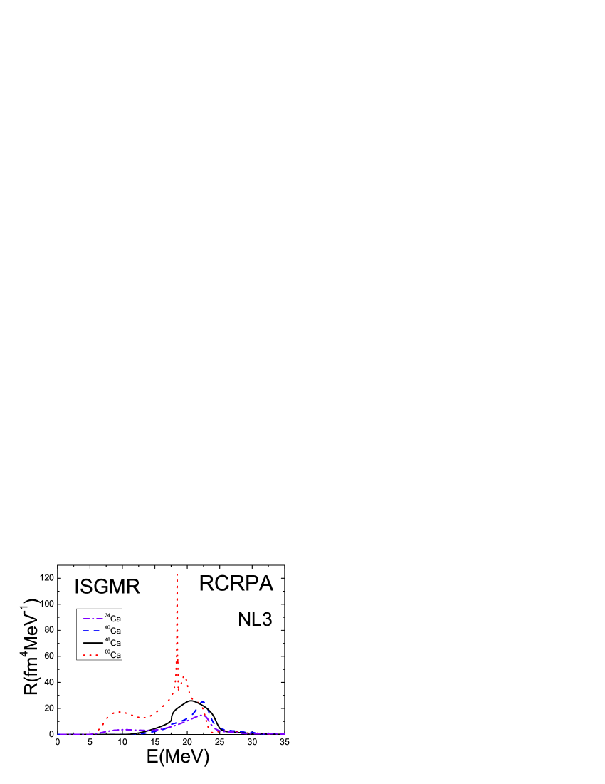
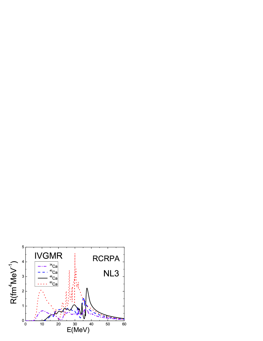
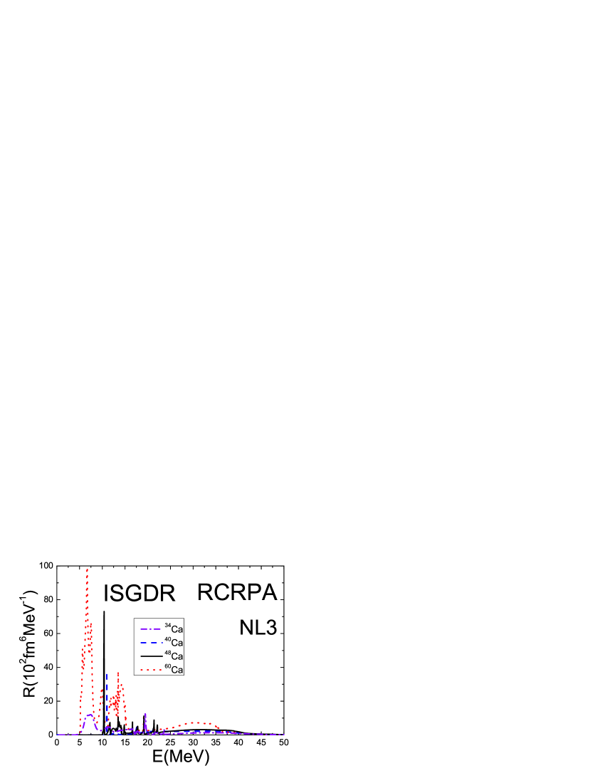
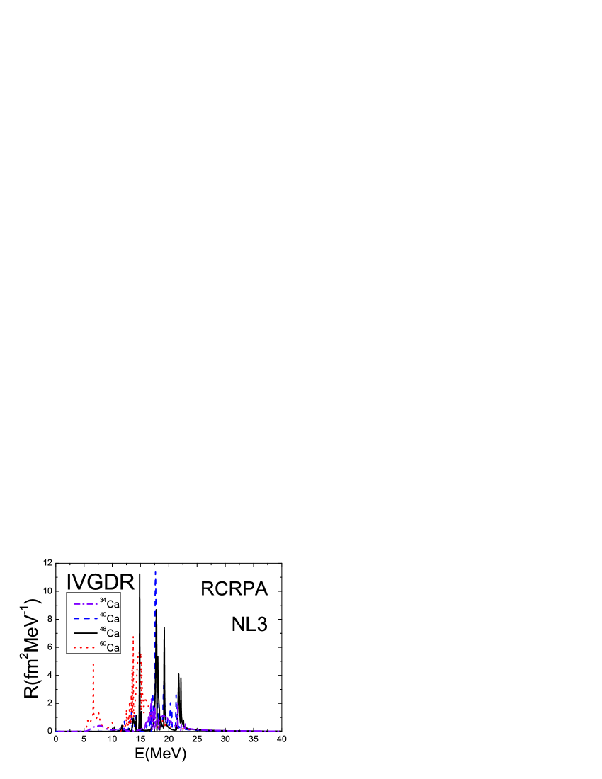
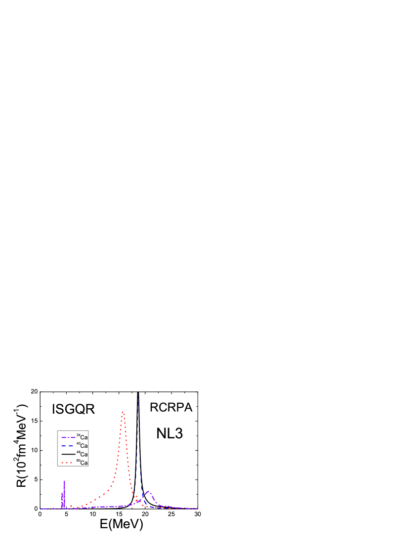
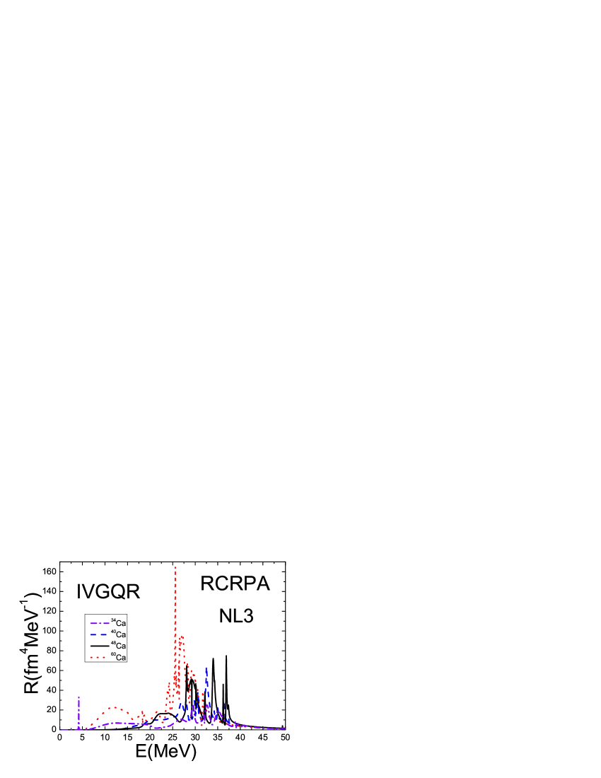
Figure 1: (color online) The response functions of ³⁴Ca, ⁴⁰Ca,⁴⁸Ca and ⁶⁰Ca in RCRPA .The dash-dotted,dashed,solid and dotted curves represent the results of ³⁴Ca, ⁴⁰Ca,⁴⁸Ca and ⁶⁰Ca, respectively.

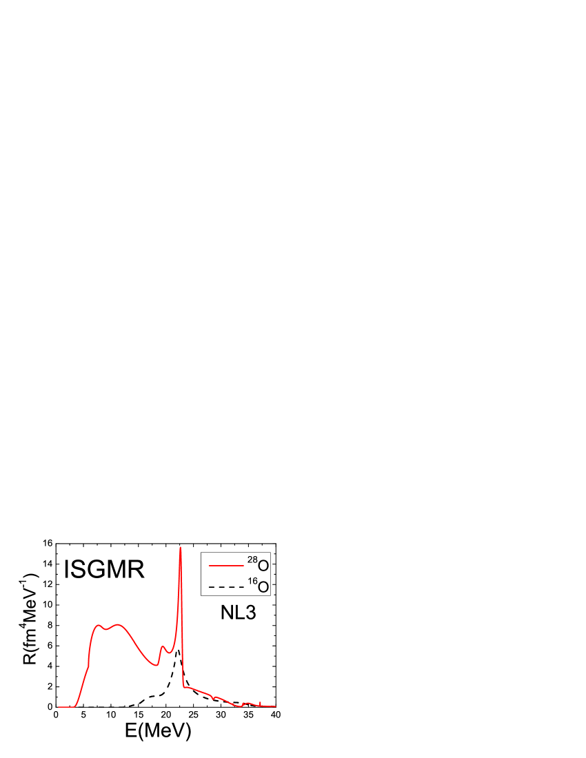
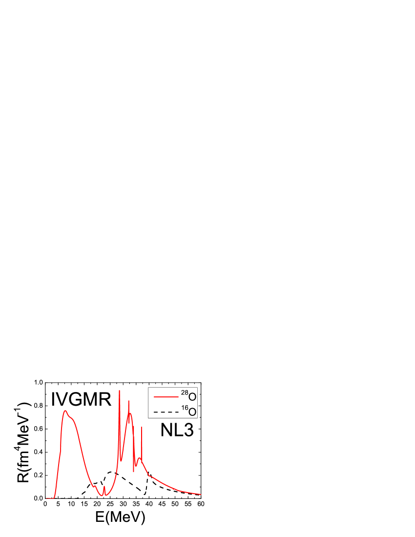
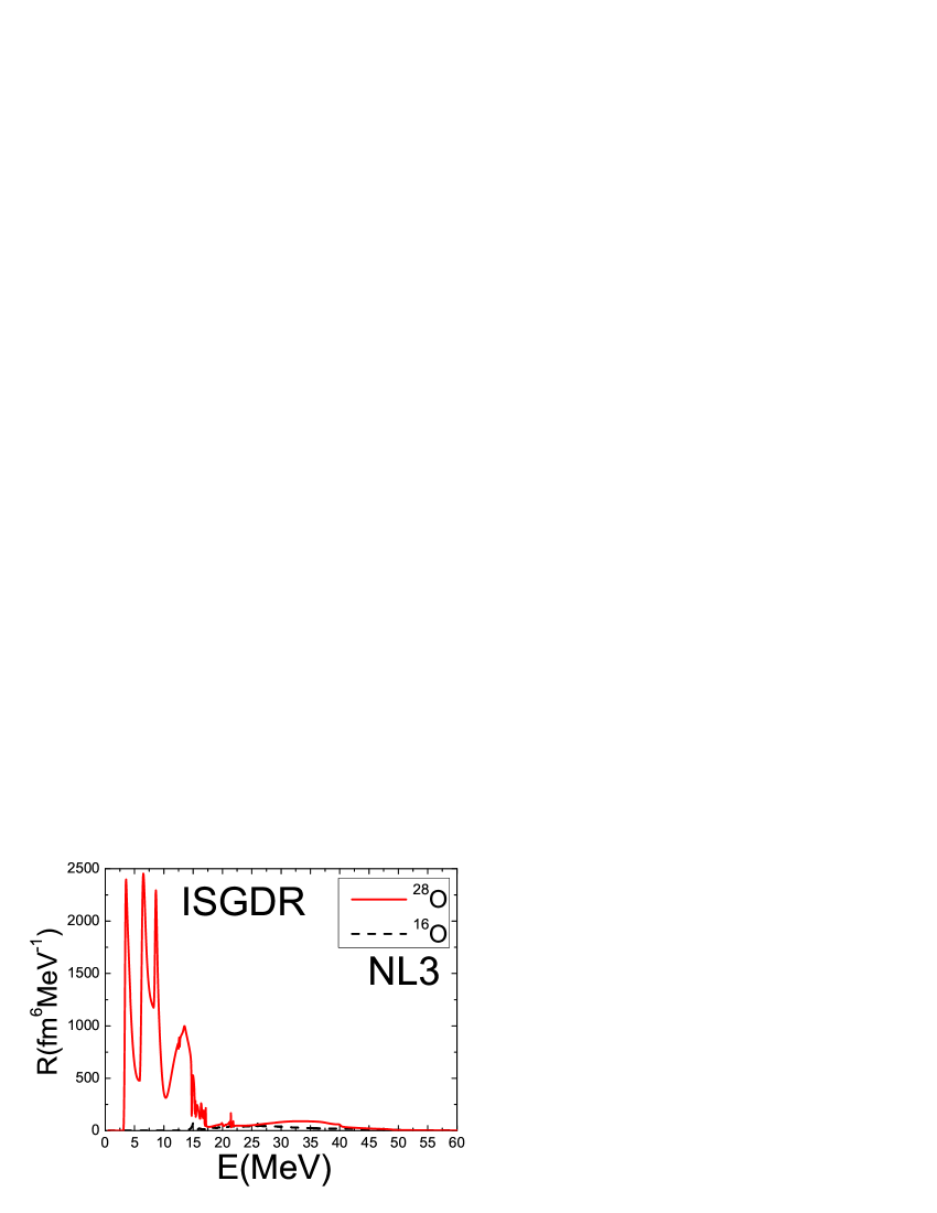
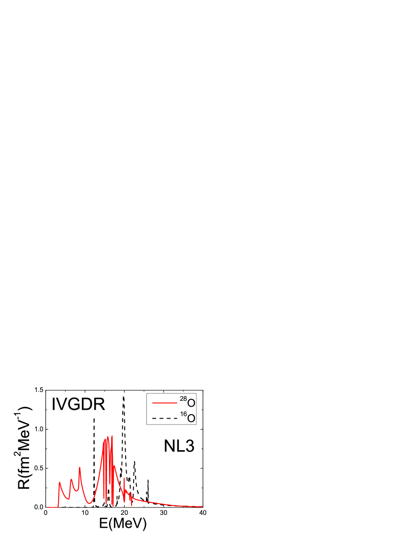
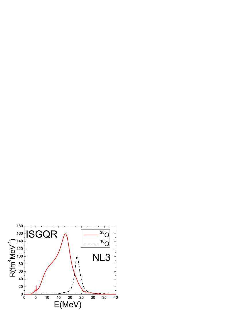
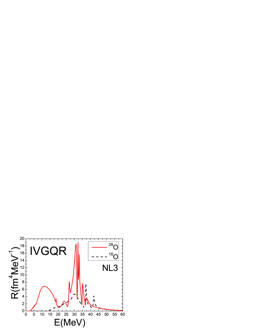
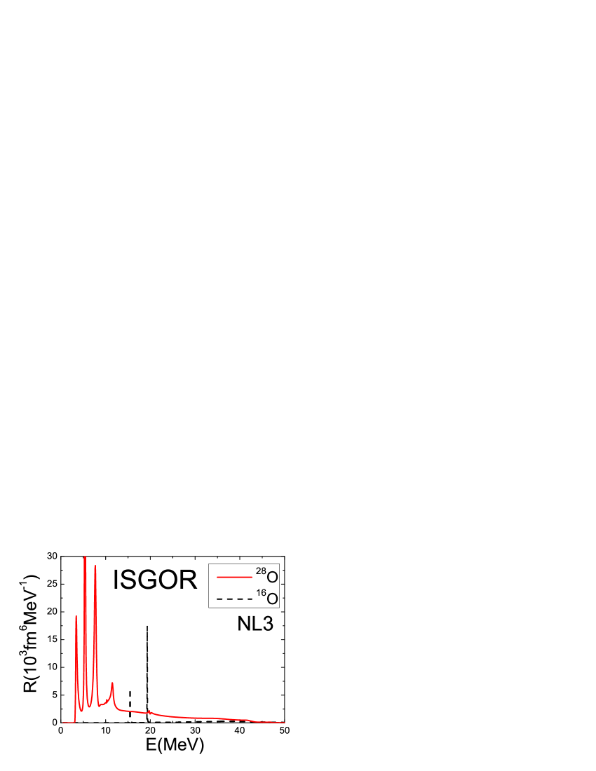
Figure 2: (color online) The response functions of ¹⁶O and ²⁸O in RCRPA .The solid and dashed curves represent the results of ²⁸O and ¹⁶O, respectively.

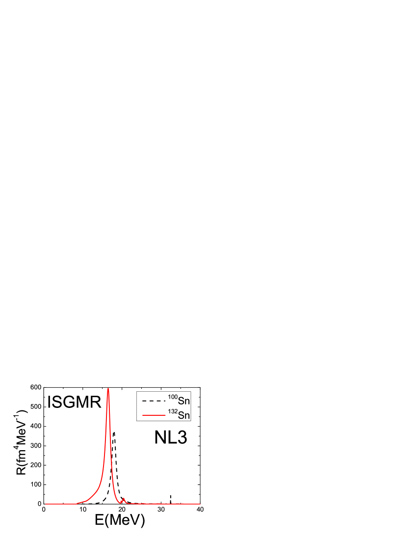
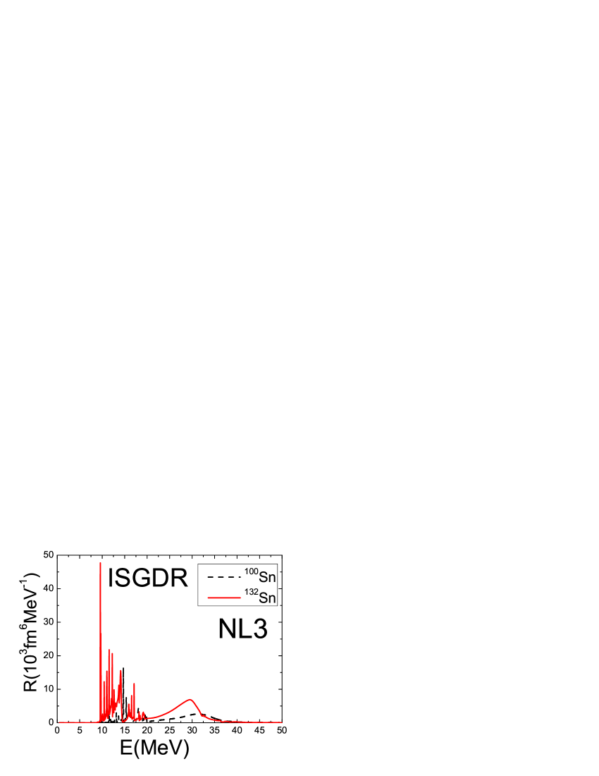
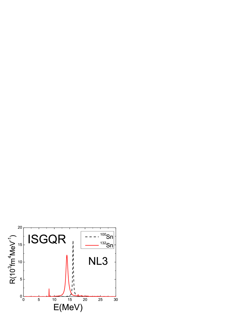
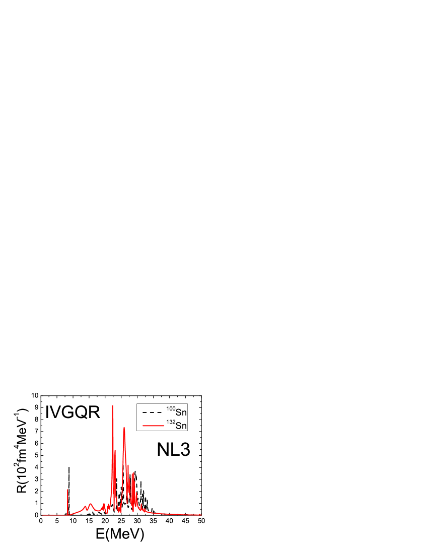
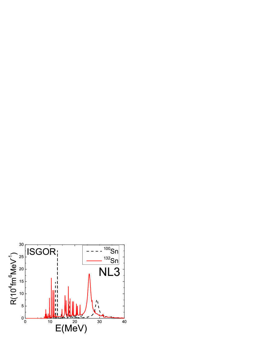
Figure 3: (color online) The response functions of ¹⁰⁰Sn and ¹³²Sn in RCRPA .The solid and dashed curves represent the results of ¹³²Sn and ¹⁰⁰Sn, respectively.

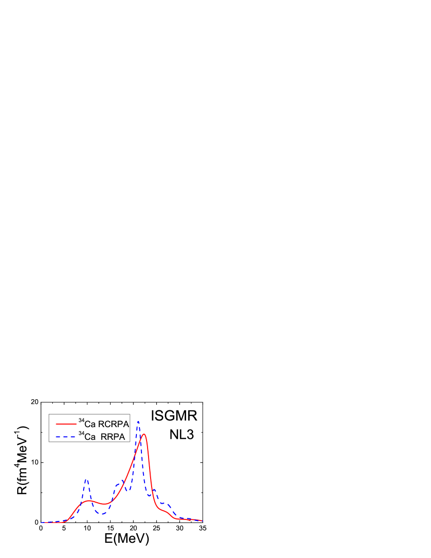
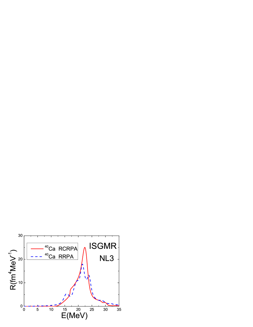
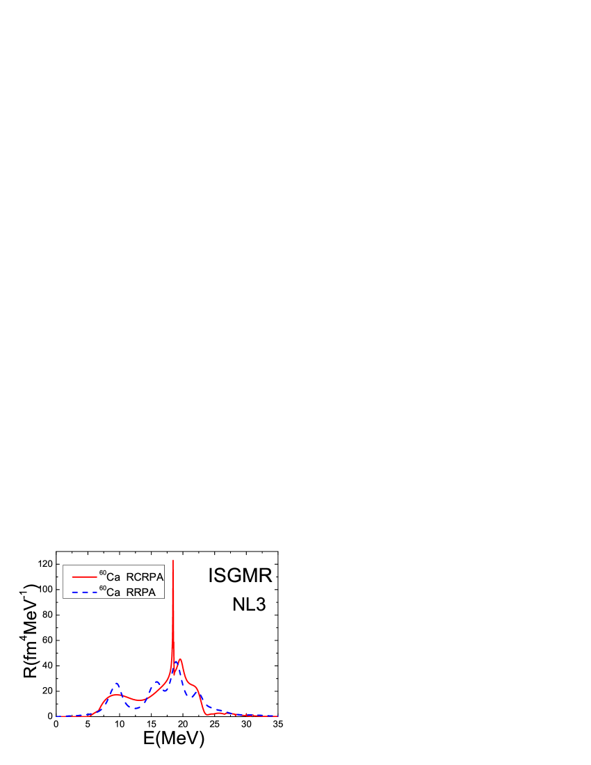
Figure 4: (color online) The ISGMR response functions of ³⁴Ca, ⁴⁰Ca,⁴⁸Ca and ⁶⁰Ca in RCRPA and RRPA.The solid and dashed curves represent the results of RCRPA and RRPA, respectively.

III Collective Multipole Excitations of Exotic Nuclei

The response functions of isoscalar and isovector giant resonances of multipolarities $L$ = 0-2 for ³⁴Ca, ⁴⁰Ca, ⁴⁸Ca and ⁶⁰Ca calculated in RCRPA are plotted in Fig.1. The dashed-dotted, dashed, solid and dotted curves represent the results of ³⁴Ca, ⁴⁰Ca, ⁴⁸Ca and ⁶⁰Ca, respectively. As we know, ⁶⁰Ca is neutron-rich nucleus and ³⁴Ca is proton-rich nucleus. In neutron-rich and proton-rich nuclei, the neutron or proton density has different profile. From Fig.1, we find that the neutron or proton excess has large effects on the energy distribution of the strength, it leads to strong low-energy excitations and pushes the centroid of the strength function to lower energies. In the isovector resonances, one observes some fragmentation in neutron-rich nucleus ⁶⁰Ca , namely, the neutron excess increases the fragmentation of the strength distribution. In contrast to response function of stable nucleus ⁴⁸Ca, in neutron-rich nucleus ⁶⁰Ca and proton-rich nucleus ³⁴Ca, strong low-energy excitations are found, especially in the case of ⁶⁰Ca. In the case of the isoscalar giant quadrupole resonance(ISGQR), it is clearly found that the response functions of the normal nuclei ⁴⁰Ca and ⁴⁸Ca are similar, in contrast, the response function of neutron-rich nucleus ⁶⁰Ca is shifted to lower-energy region remarkablely, the response function of proton-rich nucleus ³⁴Ca is separated into higher-energy region and low-energy excitations. In the compressional isoscalar giant monopole resonance(ISGMR) and isoscalar giant dipole resonance(ISGDR), a strong strength at lower energy is found in neutron-rich nucleus ⁶⁰Ca, lower-energy excitation can also be found in proton-rich nucleus ³⁴Ca, but it is smaller than that of ⁶⁰Ca. On the other hand, the higher-energy part of the strength in ⁶⁰Ca goes up, while the higher-energy part in ³⁴Ca drops down.

In addition, in order to show the above discussion is more general, we present the response functions of ¹⁶O and ²⁸O for L=0-3 calculated in RCRPA in Fig.2. The solid and dashed curves represent the results of ²⁸O and ¹⁶O, respectively. We also show the response functions of ¹⁰⁰Sn and ¹³²Sn for L=0-3 calculated in RCRPA in Fig.3. The solid and dashed curves represent the results of ¹³²Sn and ¹⁰⁰Sn, respectively. Here, ¹⁶O is a normal nucleus, and ¹⁰⁰Sn is a proton-rich nucleus, while ²⁸O and ¹³²Sn are neutron-rich nuclei. From Fig.2-3, it is also found that the neutron excess leads to strong low-energy excitations and increases the fragmentation of the strength distribution. It can be seen easily that the above results are similar to those of Ca isotopes.

It is known that the continuum in the RRPA calculations is usually discretized by the box boundary conditions, while the continuum plays important role in description of the properties of neutron-rich nuclei and proton-rich nuclei since the Fermi surface of those nuclei is close to the particle continuum, one shall treat the contribution of the continuum properly, As a result, it is required to consider the contribution of the continuum rigorously in exotic nuclei both for the ground states and excited states calculations. Finally, in order to clarify the effect of treating the contribution of continuum exactly, the ISGMR response functions given by RCRPA are compared with those obtained by RRPA. The ISGMR response functions of ³⁴Ca, ⁴⁰Ca, ⁴⁸Ca and ⁶⁰Ca given by RCRPA and RRPA are plotted in Fig.4. The solid and dashed curves represent the results of RCRPA and RRPA, respectively. From the Fig.4, it can be noted that the response functions calculated in RCRPA and RRPA are different from each other, in the case of RRPA results the width of strength functions is given artifically, in the present calculations we set it equals to 2 MeV, while it is given automatically by the RCRPA calculations, not only the Landau width but also the escaping width. For example, there is a sharp peak in the ISGMR strength of ⁶⁰Ca given by RCRPA calculation, this is mainly due to the contribution of the single-particle resonances states in the continuum, but it can not be reproduced by the RRPA calculation.

IV Summary

In conclusion, we have studied the isoscalar and isovector collective multipole excitations in exotic nuclei in the RCRPA framework. The method is based on the Green’s function technique and the contribution of the continuum spectrum is treated exactly. We have found strong low-energy excitations in neutron-rich nuclei and proton-rich nuclei which is different from the case in $\beta$-stable nuclei. Namely, the neutron or proton excess leads to strong low-energy excitations and increases the fragmentation of the strength distribution. The effects of treating the contribution of continuum exactly are also discussed.

References

• (1) N. Paar, D. Vretenar, E. Khan, and G. ColΓ³, Rep. Prog. Phys. 70, 691 (2007).
• (2) Zhong-yu Ma, N. V. Giai, A. Wandelt, D. Vretenar and P. Ring, Nucl. Phys. A686, 173 (2001); Zhong-yu Ma, Commun. Theo. Phys. 32, 493 (1999).
• (3) Zhong-yu Ma, A. Wandelt, N. V. Giai, D. Vretenar, P. Ring and Li-gang Cao,Nucl. Phys. A703, 222 (2002).
• (4) P. Ring, Zhong-yu Ma, N. V. Giai, A. Wandelt, D. Vretenar and Li-gang Cao, Nucl. Phys. A694, 249 (2001).
• (5) J. Piekarewicz, Phys. Rev. C64, 024307 (2001).
• (6) L. G. Cao and Z. Y. Ma, Eur. Phys. J. A22, 189 (2004).
• (7) Yang Ding, Cao Li-Gang, and Ma Zhong-Yu, Chin. Phys. Lett. 26 (2009)022101.
• (8) Yang Ding, Cao Li-Gang, and Ma Zhong-Yu, Commun. Theor. Phys. 53(2010) 716.
• (9) Yang Ding, Cao Li-Gang, and Ma Zhong-Yu, Commun. Theor. Phys. 53(2010) 723.
• (10) Yang Ding, Cao Li-Gang, Tian Yuan and Ma Zhong-Yu, Phys. Rev. C82, 054305 (2010).