Segmentation procedure based on Fisher’s exact test and its application to foreign exchange rates

Abstract

This study proposes the segmentation procedure of univariate time series based on Fisher’s exact test. We show that an adequate change point can be detected as the minimum value of p-value. It is shown that the proposed procedure can detect change points for an artificial time series. We apply the proposed method to find segments of the foreign exchange rates recursively. It is also applied to randomly shuffled time series. It concludes that the randomly shuffled data can be used as a level to determine the null hypothesis.

1 Introduction

Recently researchers on data analysis have paid significant attention to change–points detection. This is a problem to find an adequate change–points from nonstationary time series. One faces this problem when treating data on socio-economic-environmental systems.

The literature on change–point detection is rather huge: reference monographs include Basseville and Nikiforov [3], Brodsky and Darkhovsky [4], Csörgő and Horváth [5], Chen and Gupta [6]. The journal articles by Giraitis and Leipus [7, 8], Hawkins [9, 10], Chen and Gupta [11], Mia and Zhao [12], Sen and Srivastava [13] among others, are also of interest.

There are two types of approaches to segmentation procedure. One is a local approach and another is a global approach. Lavielle and Teyssière [14] addressed the issue of global procedure vs local procedure, and found that the extension of single change–points procedures to the case of multiple change–point using Vostrikovaś [15] binary segmentation procedure is misleading and yields an overestimation of the number of change–points. Quantdt and Ramsey have developed estimation procedure for mixture of linear regression [1]. Kawahara and Sugiyama [16] propose a non-parametric method to detect change points from time series based on direct density–ratio estimation. More recently, a recursive entropic scheme to separate financial time series has been proposed [17]. Their method is parametric and uses the log–likelihood ratio test.

Decré-Robitaille et al.  [18] compare several methods to detect change points. They segment artificial time series based on 8 methods; standard normal homogeneity test (SNHT) without trend [19], SNHT with trend [20], multiple linear regression (MLR) [21], two-phase regression (TPR) [22], Wilcoxon rank-sum (WRS) [23], sequential testing for equality of means (ST) [24], Bayesian approach without reference series [25, 26], and Bayesian approach with reference series [25, 26]. Karl and Williams [23] propose a method to find an adequate segment boundary based on Wilcoxon rank–sum test and investigate climatological time series data.

We further address some existing approaches to the problem of multiple change–point detection in multivariate time series. Ombao et al. [27] employ the SLEX (smooth localized complex exponentials) basis for time series segmentation, originally proposed by Ombao et al. [28]. The choice of SLEX basis leads to the segmentation of the time series, achieved via complexity–penalized optimization. Lavielle and Teyssière [29] introduce a procedure based on penalized Gaussian log–likelihood as a cost function, where the estimator is computed via dynamic programming. The performance of the method is tested on bivariate examples. Vert and Bleakley [30] propose a method for approximating multiple signals (with independent noise) via piecewise constant functions, where the change-point detection problem is re-formulated as a penalized regression problem and solved by the group Lasso [31]. Note that Cho and Fryzlewicz [32] argue that Lasso-type penalties are sub-optimal for change-point detection.

In this study, we propose a non-parametric method to detect an adequate segment boundary. Our procedure is based on Fisher’s exact test and uses it as a discriminant measure to detect the segmentation boundary. Fisher’s exact test can be used in the case of a small number of samples. The proposed method is performed with both artificial nonstationary time series and actual data on daily log–return time series.

This paper is organized as follows. We introduce Fisher’s exact test and propose a non-parametric method to find an adequate change point from time series in Section 2. We perform the proposed method with artificial nonstationary time series in Section 3. We conduct empirical analysis of the daily log–return time series of AUD/JPY in Section 4. Section 5 is devoted to conclusions.

2 Fisher exact test for segmentation procedure

We want to find an adequate segment regarding non-stationarity of $r(t)$. Assume that the time series $r(t)$ consists of $n$ segments. The problem is to determine $n-1$ boundaries from the time series.

Firstly, we discuss a method to determine an adequate boundary in a time series based on Fisher’s exact test. Introducing $x_{th}$ in a value and $\tau$ in time, we count the number of four events:

• $a$ : the number of $r(t)>x_{th}$ for $0\leq t<\tau$.

• $b$ : the number of $r(t)\leq x_{th}$ for $0\leq t<\tau$.

• $c$ : the number of $r(t)>x_{th}$ for $\tau<t\leq T$.

• $d$ : the number of $r(t)\leq x_{th}$ for $\tau<t\leq T$.

According to Fisher’s exact test, fixing the vertical numbers $a+c$ and $b+d$, horizontal numbers $a+b$ and $c+d$, the two-sided probability of $2\times 2$ matrix $\left[\begin{array}[]{cc}a&b\\ c&d\end{array}\right]$ is given as

$$p(a,b,c,d)=\frac{\sum_{i=0}^{\mbox{min}(b,c)}(_{a+c}C_{c-i}\cdot_{b+d}C_{b-i})+\sum_{i=0}^{\mbox{min}(a,d)}(_{a+c}C_{a-i}\cdot_{b+d}C_{d-i})}{{}_{n}C_{a+b}}$$ (1)

This probability is used as p-value for realized quartet $(a,b,c,d)$. The smallest p-value tells us that the threshold $x_{th}$ and the boundary $\tau$ are of statistically significance. Therefore, we can detect a change point from the minimization problem;

$$\{\hat{\tau},\hat{x}_{th}\}=\arg\min_{\tau,x_{th}}p\Bigl{(}a(\tau,x_{th}),b(\tau,x_{th}),c(\tau,x_{th}),d(\tau,x_{th})\Bigr{)}.$$ (2)

If the minimum p-value for the event which we observed as the quartet $(a,b,c,d)$ is less than a certain significance level $p_{th}$, then the event is regarded as a statistically significant case and the boundary $\tau$ should be accepted as a change–point.

Let us now briefly discuss some issues related to the determination of $\hat{\tau}$. The interpretation of this time point $\hat{\tau}$ is that it gives an optimal separation of the time series into two statistically most distinct segments. The segmentation procedure can be used recursively to separate further the segmented time series into smaller segments. We do this iteratively until the iteration is terminated by a stopping condition. Several termination conditions have been proposed in previous studies. We terminate the iteration if the p-value is larger than the amplitudes of typical fluctuations in the spectra.

In practice, in order to simplify the recursive segmentation, we adopt a conservative threshold of $p_{th}$ and terminate the procedure if $p(a,b,c,d)$ is less than $p_{th}$.

3 Numerical Study

As artificial nonstationary time series, we generate time series as the following algorithm.

$$x(t)=\left\{\begin{array}[]{ll}\sigma\xi(t)&1\leq t\leq 50\\ \sigma\xi(t)+0.1&51\leq t\leq 150\\ \end{array}\right.,$$ (3)

where $\xi(t)$ is drawn from i.i.d. standard normal distribution with zero mean, and standard deviation $\sigma$. Fig. 1 shows a sample of artificial nonstationary time series with $\sigma=0.01$, $0.05$, and $0.1$. These time series are generated from the same random seed.

We compute the minimum p-value varying the value of $\sigma$. Fig. 2 shows the relationship between the minimum p-value and $\sigma$. As $\sigma$ increases, the minimum p-value increases. Namely, the estimation error for change points increases as $\sigma$ increases. In this case, statistically significant estimation of the change point is given for $\sigma<0.1$. This implies that a point where the minimum p-value is less than $10^{-5}$ is statistically significant.

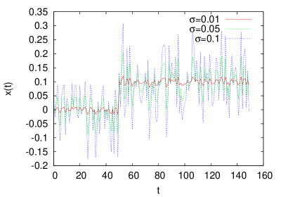
Figure 1: Artificial nonstationary time series at $\sigma=0.01$, $0.05$, and $0.1$ with the same random seed.

(a) (b)

Figure 2: (a) The relationship between $\sigma$ and the minimum p-value. Each curve corresponds to the relationship between $\sigma$ and the minimum p-value computed from the artificial time series with the same random seed. (b) The points giving the minimum p-value at $\sigma$. Each curve corresponds to the relationship between $\sigma$ and the estimated change point.

As artificial nonstationary time series, we generate another type of time series as the following algorithm.

$$x(t)=\left\{\begin{array}[]{ll}\sigma\xi(t)&1\leq t\leq 50\\ \sigma\xi(t)+0.001(t-50)&51\leq t\leq 150\\ \end{array}\right.,$$ (4)

where $\xi(t)$ is drawn from i.i.d. standard normal distribution with zero mean, and standard deviation $\sigma$. Fig. 3 shows artificial nonstationary time series with $\sigma=0.01$, $0.05$, and $0.1$. These time series are generated from the same random seed.

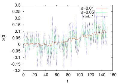
Figure 3: Artificial nonstationary time series at $\sigma=0.01$, $0.05$, and $0.1$ with the same random seed.

(a) (b)

Figure 4: (a) The relationship between $\sigma$ and the minimum p-value. Each curve corresponds to the relationship between $\sigma$ and the minimum p-value computed from the artificial time series with the same random seed. (b) The points giving the minimum p-value at $\sigma$. Each curve corresponds to the relationship between $\sigma$ and the estimated change point.

We compute the minimum p-value varying the value of $\sigma$. Fig. 4 shows the relationship between the minimum p-value and $\sigma$. As $\sigma$ increases, the minimum p-value increases. Namely, the estimation error for change points increases as $\sigma$ increases. In this case, statistically significant estimation of the change point is given for $\sigma<0.2$. This implies that a point where the minimum p-value is less than $10^{-5}$ is statistically significant.

Comparing p-values from two examples, p-values shown in Fig. 2 show smaller values than those in Fig. 4. The error sensitivity depends on the type of nonstationarity.

4 Empirical Analysis

We apply a recursive segmentation procedure with our proposed method to an actual time series. We use daily log–return time series of foreign exchange rate of Australian Dollar (AUD) against Japanese Yen (JPY). The log–return time series of AUD/JPY for the period from 03 January, 2001 to 30 December, 2011. Throughout this analysis, we set the threshold as $p_{th}=10^{-5}$.

Suppose that $R(t)$ represents an exchange rate at business day $t\quad(t=1,\ldots,n+1)$. Let $r(t)$ be a daily log–return of exchange rate at time $t\quad(t=1,\ldots,n)$, which is defined as $r(t)=\log R(t+1)-\log R(t)$. Following the procedure shown in Sec. 2, we count the number of four events and compute the p-value.

Fig. 5 shows exchange rates of AUD/JPY, their daily log–return time series, and the p-value computed from Fisher’ exact test. We compute the minimum p-value changing $x_{th}$ from Eq. (1) on business day $\tau$. From Fig. 5 (c) we observe the smallest p-value, which is estimated as $2.6\times 10^{-27}$, on 22 June, 2007. Since the smallest p-value is less than $p_{th}=10^{-5}$, we determine this date as an adequate boundary. Repeating to apply this procedure to each two segments, we obtain all the segments until the smallest p-value is greater than $p_{th}$. We detect six segments in the time series and show sample mean and sample standard deviation computed from each segment in Tab. 1.

Suppose that we have $K$ segments. Let $[t_{k-1}+1,\ldots,t_{k}]$ represent a range of the $k$-th segment ($t_{0}=0$). The mean value of the $k$-th segment is computed as

$$\mu^{(k)}=\frac{1}{t_{k}-t_{k-1}}\sum_{t=t_{k-1}+1}^{t_{k}}r(t).$$ (5)

We attempt to obtain an adequate fitting curve in each segment based on each estimated segment. Since we can describe $R(t+1)=R(t)\exp\bigl{(}r(t)\bigr{)}$ of exchange rate $R(t)$ at business time $t$, we assume that the exchange rate is fitted with

$$R(t)=\exp\Bigl{(}\mu^{(k)}(t-t_{k-1})+\rho\Bigr{)}\quad(t_{k-1}+1\leq t\leq t_{k}),$$ (6)

The value $\rho$ is estimated with the least squared method:

$$\rho=\frac{1}{t_{k}-t_{k-1}}\sum_{t=t_{k-1}+1}^{t_{k}}\Bigl{(}\log R(t)-\mu(t-t_{k-1})\Bigr{)}$$ (7)

We can compute parameter $\rho$ of this simple regression model from time series. The detail derivation of Eq. (7) is described in A.

A positive trend of AUD against JPY reveals in both the first and second segments. In the third segment AUD against JPY drops slightly and in the fourth segment the exchange rates of AUD against JPY steeply drops due to the influence of global financial crisis driven by the Lehman shock. In both the fifth and sixth segments the exchange rates of AUD/JPY are eventually stabilized and volatility decreases. Fig. 6 shows the segments detected with the proposed method. The first and second segments are related to a growth phase in the world economy. In the third segment, we observed instability of the global economy. The fourth segment coincides the global financial crisis triggered by bankruptcy of Lehman brothers in September 2008. After the Lehman shock, JPY rapidly dropped against AUD.

We generate randomly shuffled data from the log–return time series. The randomly shuffled data preserves sample mean and sample standard deviation of original time series. We compute p-value for the randomly shuffled data with the proposed method. Fig. 7 (a) shows the randomly shuffled time series, and (b) p-value computed for the randomly shuffled data. The p-value is almost always larger than $10^{-2}$. This implies that the p-value of original time series is more statistically significant than randomly shuffled data.

Table 1: Descriptive statistics of each segment.

no.	start	end	mean	std.
1	2001-1-3	2002-2-8	0.000253	0.009131
2	2002-2-11	2007-6-21	0.000312	0.006308
3	2007-6-22	2008-9-11	-0.000676	0.012243
4	2008-9-12	2008-12-8	-0.005385	0.042808
5	2008-12-9	2009-7-8	0.001095	0.018160
6	2009-7-9	2011-12-30	0.000141	0.010740

(a) (b) (c)

Figure 5: (a) Daily exchange rates of AUD/JPY, (b) daily log return time series of AUD/JPY, (c) the p-value computed from the daily log–return time series of AUD/JPY with Fisher exact.

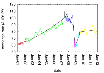
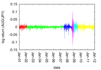
(a) (b)

Figure 6: (a) Daily exchange rates of AUD/JPY segmented by the recursive Fisher Exact test and (b) segmented daily log return of AUD/JPY.

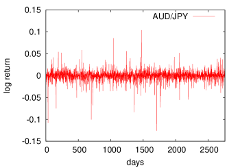
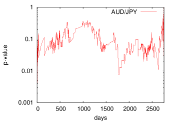
(b) (c)

Figure 7: (a) Randomized daily log return time series of AUD/JPY, and (b) the p-value computed from daily log return time series.

5 Conclusion

This paper proposed the segmentation procedure based on Fisher’s exact test. The proposed method was tested for artificial time series. It was confirmed that the ratio of mean values of time series to their volatility is associated with the estimation error of segmentation boundary. As the variance increases, the estimation error increases. The proposed method was applied to the actual data of daily foreign exchange rates. The change points detected with the proposed method were characterized in terms of sample mean and standard deviations of daily log–return time series. The randomly shuffled data was used as the null hypothesis. The shuffled data showed the large p-value which can not be accepted as a segmentation boundary.

Appendix A Derivation of the price fitting curve

Assume that $R(t)\quad(t=1,\ldots,n+1)$ is divided into $K$ segments. The $k$-th segment takes a range from $t_{k-1}+1$ to $t_{k}$, where $t_{0}=0$ and $t_{K+1}=n+1$. Suppose the fitting curve of the $k$-th segment of exchange rate $R(t)\quad(t=t_{k-1}+1,\ldots,t_{k})$ as

$$R(t)=\exp\Bigl{(}\mu(t-t_{k-1})+\rho\Bigr{)}.$$ (8)

We assume that the least squared error can be written as

$$E(\rho)=\sum_{t=t_{k-1}+1}^{t_{k}}\Bigl{(}\log R(t)-\mu(t-t_{k-1})-\rho\Bigr{)}^{2}.$$ (9)

Differentiating $E(\rho)$ in terms of $\rho$ and setting it into zero, we get

$$2\sum_{t=t_{k-1}+1}^{t_{k}}\Bigl{(}\log R(t)-\mu(t-t_{k-1})-\rho\Bigr{)}=0.$$ (10)

Consequently, we obtain

$$\rho=\frac{1}{t_{k}-t_{k-1}}\sum_{t=t_{k-1}+1}^{t_{k}}\Bigl{(}\log R(t)-\mu(t-t_{k-1})\Bigr{)}.$$

References

- [1] Quandt, R.E. and Ramsey, J.B., 1978. Estimating Mixtures of Normal Distributions and Switching Regressions. Journal of the American Statistical Association. 73, 730–738.
- [2] Achcar, J.A. and Loibel, S., 1998. Constant Hazard Function Models with a Change Point: A Bayesian Analysis Using Markov Chain Monte Carlo Methods. Biometrical Journal. 40, 543–555.
- [3] Basseville, M. and Nikiforov, N., 1993. The Detection of Abrupt Changes - Theory and Applications, Prentice-Hall, New Jersey.
- [4] Brodsky, B. and Darkhovsky, B., 1993. Nonparametric Methods in Change–Point Problems, Kluwer Academic Publishers, Dordrecht
- [5] Csörgő, M. and Horváth, L., 1997. Limit Theorems in Change–Point Analysis, Wiley, Chichester
- [6] Chen, J. and Gupta, A.K., 2000. Parametric Statistical Change Point Analysis, Birkhäuser, Basel.
- [7] Giraitis, L. and Leipus, R., 1992. Testing and estimating in the change–point problem of the spectral function, Lithuanian Mathematical Journal, 32, 15–29.
- [8] Giraitis, L. and Leipus, R., 1990. Functional CLT for nonparametric estimates of the spectrum and change–point problem for a spectral function, Lithuanian Mathematical Journal, 30, 674–679.
- [9] Hawkins, D.M., 1977. Testing a sequence of observations for a shift in location, Journal of the American Statistical Association, 72, 180–186.
- [10] Hawkins, D.M., 2001. Fitting multiple change–point models to data, Computational Statistics and Data Analysis, 37, 323–341.
- [11] Chen, J. and Gupta, A.K., 2004. Statistical inference of covariance change points in Gaussian models, Statistics, 38, 17–28.
- [12] Mia, B.Q. and Zhao, L.C., 1988. Detection of change points using rank methods. Communications in Statistics - Theory and Methods, 17, 3207–3217.
- [13] Sen, A. and Srivastava, M.S., 1975. On tests for detecting change in the mean, The Annals of Statistics, 3, 96–103.
- [14] Lavielle, M. and Teyssière, G., 2005. Adaptive detection of multiple change–points in asset price volatility, in: G. Teyssière and A. Kirman (Eds.), Long–Memory in Economics, 129–156. Springer Verlag, Berlin.
- [15] L. Ju. Vostrikova, 1981. Detection of disorder in multidimensional random processes, Soviet Mathematics Doklady, 24, 55–59.
- [16] Kawahara, Y. and Sugiyama, M., 2012. Sequential change-point detection based on direct density–ratio estimation, Statistical Analysis and Data Mining, 5, 114–127.
- [17] Cheong, S.A. et. al., 2012. The Japanese economy in crises: A time series segmentation study, Economics E-journal, 2012-5, on http://www.economics-ejournal.org.
- [18] Ducré-Robitaille, J.-F., Vincent, L.A. and Boulet, G., 2003. Comparison of techniques for detection of discontinuities in temperature series, International Journal of Climatology, 23, 1087–1101.
- [19] Alexandersson, H., 1986. A homogeneity test applied to precipitation data, Journal of Climatology, 6, 661–675.
- [20] Alexandersson, H. and Moberg, A., 1997. Homogenization of Swedish temperature data. Part I: homogeneity test for linear trends, International Journal of Climatology, 17, 25–34.
- [21] Vincent, L.A., 1998. A technique for the identification of inhomogeneities in Canadian temperature series, Journal of Climate, 11, 1094–1104.
- [22] Easterling, D.R. and Peterson, T.C., 1995. A new method for detecting undocumented discontinuities in climatological time series. International, Journal of Climatology, 15, 369–377.
- [23] Karl, T.R. and Williams, Jr C.N., 1987. An approach to adjusting climatological time series for discontinuous inhomogeneities, Journal of Climate and Applied Meteorology, 26, 1744–1763.
- [24] Gullett, D.W., Vincent, L., Sajecki, P.J.F., 1990. Testing homogeneity in temperature series at Canadian climate stations, CCC report 90-4, Climate Research Branch, Meteorological Service of Canada, Ontario, Canada.
- [25] Perreault, L., Haché, M., Slivitsky, M. and Bobée, B., 1999. Detection of changes in precipitation and runoff over eastern Canada and US using a Bayesian approach, Stochastic Environmental Research and Risk Assessment, 13, 201–216.
- [26] Perreault, L., Bernier, J., Bobée, B., and Parent, E., 2000. Bayesian change-point analysis in hydrometeorological time series. Part 1. The normal model revisited, Journal of Hydrology, 235, 221–241.
- [27] Ombao, H., Sachs, R. von, and Guo, W., 2005. SLEX analysis of multivariate nonstationary time series, Journal of the American Statistical Association, 100, 519–531.
- [28] Ombao, H., Raz, J.A. Sachs, R. von and Guo, W., 2002. The SLEX model of a non-stationary random process, Annals of the Institute of Statistical Mathematics, 54, 171–200.
- [29] Lavielle, M. and Teyssière, G., 2006. Detection of multiple change-points in multivariate time series, Lithuanian Mathematical Journal, 46, 287–306.
- [30] Vert, J. and Bleakley, K., 2010. Fast detection of multiple change-points shared by many signals using group LARS, Advances in Neural Information Processing Systems, 23, 2343–2351.
- [31] Yuan, M. and Lin, Y., 2006. Model selection and estimation in regression with grouped variables, Journal of the Royal Statistical Society, Series B, 68, 49–67.
- [32] Cho, H. and Fryzlewicz, P., 2011. Multiscale interpretation of taut string estimation and its connection to Unbalanced Haar wavelets, Statistics and Computing, 21, 671–681.