Cascade of minimizers for a nonlocal isoperimetric problem in thin domains

Abstract

For $\Omega_{\varepsilon}=(0,\varepsilon)\times(0,1)$ a thin rectangle, we consider minimization of the two-dimensional nonlocal isoperimetric problem given by

$$\inf_{u}E^{\gamma}_{\Omega_{\varepsilon}}(u)$$

where

$$E^{\gamma}_{\Omega_{\varepsilon}}(u):=P_{\Omega_{\varepsilon}}(\{u(x)=1\})+\gamma\int_{\Omega_{\varepsilon}}\left|{\nabla{v}}\right|^{2}\,dx$$

and the minimization is taken over competitors $u\in BV(\Omega_{\varepsilon};\{\pm 1\})$ satisfying a mass constraint $\fint_{\Omega_{\varepsilon}}u=m$ for some $m\in(-1,1)$. Here $P_{\Omega_{\varepsilon}}(\{u(x)=1\})$ denotes the perimeter of the set $\{u(x)=1\}$ in $\Omega_{\varepsilon}$, $\fint$ denotes the integral average and $v$ denotes the solution to the Poisson problem

$$-\Delta v=u-m\;\mbox{in}\;\Omega_{\varepsilon},\quad\nabla v\cdot n_{\partial\Omega_{\varepsilon}}=0\;\mbox{on}\;\partial\Omega_{\varepsilon},\quad\int_{\Omega_{\varepsilon}}v=0.$$

We show that a striped pattern is the minimizer for $\varepsilon\ll 1$ with the number of stripes growing like $\gamma^{1/3}$ as $\gamma\to\infty.$ In the process, we show that stable lamellar patterns are in fact $L^{1}$ local minimizers in rectangular domains. We then present generalizations of this result to higher dimensions.

Mathematics Subject Classification: 49J45, 49Q20
Keywords: nonlocal isoperimetric, global minimizers

1 Introduction

In nonlocal isoperimetric problems currently of interest, one considers a perturbation of the classical isoperimetric problem by a term that favors high oscillation. This tension between terms favoring low and high surface area respectively leads to a rich and not well understood energy landscape. To date, identification of minimizers has been largely limited to parameter regimes in which the perimeter term dominates and so it is the purpose of this article to present a setting, namely thin domains, that allows for such an identification at all magnitudes of the nonlocal perturbation.

To state our problem precisely, given a bounded domain $\Omega\subset\mathbb{R}^{n}$ and a number $\gamma\geqslant 0$ we consider the minimization of the functional

$$E^{\gamma}_{\Omega}(u):=P_{\Omega}(\{u(x)=1\})+\gamma\int_{\Omega}\left|{\nabla{v}}\right|^{2}\,dx$$ (1.1)

over the set of competitors $u\in BV(\Omega;\{\pm 1\})$ satisfying the mass constraint $\fint_{\Omega}u=m$ for some $m\in(-1,1)$. Here $P_{\Omega}(\{u(x)=1\})$ denotes the perimeter of the set $\{u(x)=1\}$ in $\Omega$, $\fint$ denotes the integral average and $v$ denotes the solution to the Poisson problem

$$-\Delta v=u-m\;\mbox{in}\;\Omega,\quad\nabla v\cdot n_{\partial\Omega}=0\;\mbox{on}\;\partial\Omega,\quad\int_{\Omega}v=0,$$ (1.2)

with $n_{\partial\Omega}$ denoting the outer unit normal to $\partial\Omega$. We recall that $P_{\Omega}(\{u(x)=1\})$ can alternatively be expressed as $\frac{1}{2}\left|{\nabla u}\right|(\Omega)$ where $\left|{\nabla u}\right|(\Omega)$ denotes the total variation of the vector-valued measure $\nabla u$, cf. [12].

The functional $E^{\gamma}_{\Omega}$ arises as the sharp interface $\Gamma$-limit as $\delta\to 0$ of the Ohta-Kawasaki functional modeling phase separation in diblock co-polymers

$$u\mapsto\int_{\Omega}\frac{1}{\delta}(u^{2}-1)^{2}+\delta\left|{\nabla u}\right|^{2}+\gamma\int_{\Omega}\left|{\nabla{v}}\right|^{2}\,dx,$$

see e.g. [7, 21, 24]. Thus, at least on a qualitative level, one expects that minimizers of (1.1) should bear some resemblance to the pictures of phase separation reported experimentally in the co-polymer literature, e.g. in [2, 4, 31]. The most striking feature of these images in parameter regimes where the nonlocality dominates is the emergence of small periodically arrayed cells inside of which the interface $\partial\{u=1\}$ resembles a constant mean curvature surface.

Now as we show in Section 3, and as was already studied earlier in e.g. [23] and [24], in one dimension when $\Omega$ is simply an interval, the problem can be explicitly solved. Here it is easy to see that minimizers are essentially periodic–up to adjustments at the boundary to accommodate the Neumann boundary conditions–with oscillations on the order of $\gamma^{1/3}$ in the regime $\gamma\gg 1$, a scaling that has previously been noted for example in [19]. (A similar conclusion for one-dimensional minimizers of the Ohta-Kawasaki functional can also be drawn but this is nontrivial, see [18].) When $n\geqslant 2$ however, the problem becomes quite subtle. To date, the only general result in this direction is that of [3] where the authors show, roughly speaking, that energy tends to distribute uniformly in two dimensions. A corresponding result for Ohta-Kawasaki was obtained more recently in [28].

With regard to characterizing more precisely the global minimizer, progress up to now has been largely limited to parameter regimes where perimeter dominates. When $\gamma$ is small this includes [29, 30]. There is also a growing literature on asymptotic regimes where $m$ is near $1$ or $-1$, on the setting $\Omega=\mathbb{R}^{n}$ and on related perturbations of the isoperimetric problem, some of which arise as $\Gamma$-limits of Ohta-Kawasaki under different scalings, see for example [5, 6, 9, 10, 11, 13, 15, 16, 20, 22]. In a different vein, the existence of increasingly intricate critical points and local minimizers for (1.1) and related nonlocal sharp interface problems has been one thrust of the research program of Ren and Wei, see for example [24, 26, 27] and the references therein.

In this article we investigate a multi-dimensional setting where we can identify the global minimizer of (1.1) for all values of $\gamma$. The simplest such example is the case where $\Omega$ is a thin rectangle given by $\Omega_{\varepsilon}:=(0,\varepsilon)\times(0,1)$ for $\varepsilon$ small. Our main result here, Theorem 5.4, states that for any value of $\gamma$, when $\varepsilon$ is sufficiently small, the global minimizer of $E^{\gamma}_{\Omega_{\varepsilon}}$ coincides with the minimizer of the one-dimensional problem posed on the unit interval. Since the one-dimensional problem is minimized by a piecewise constant function with more and more jumps in the regime $\gamma\gg 1$, this implies that as $\gamma$ grows the minimizer of the two-dimensional problem exhibits a cascade of oscillations through a pattern of more and more horizontal stripes. The relationship between the number of stripes $k$ and the value of $\gamma$ is given explicitly in (3.8). We then apply the technique to cover domains of the form $(0,\varepsilon)^{\ell}\times(0,1)$ for any positive integer $\ell$ and more general thin domains in Theorems 6.1 and 6.3.

Let us describe the main ingredients in the method of proof for the main result, Theorem 5.4. A first step is the establishing of $\Gamma$-convergence of (1.1) to a one-dimensional energy in the setting where $\Omega=\Omega_{\varepsilon}$ as $\varepsilon\to 0.$ This is accomplished in Section 2. Section 3 contains the explicit identification of the global minimizer of the one-dimensional $\Gamma$-limit alluded to earlier. In Section 4 we give a proof of the two-dimensional stability of the one-dimensional minimizers. This stability was first addressed in the periodic setting in [19], in which a more general machinery was introduced for studying stability of critical points in a variety of regimes, including higher dimensions. Through reflection, this yields stability for the Neumann problem of our setting. However, we include our proof here both for the stake of self-containment and because our argument is completely different from the earlier one and we find it to be quite a bit simpler. In Section 5 we first establish the appropriate modifications of the stability $\implies$ local minimality results of [1] and [14] to this setting of Neumann boundary conditions in domains with corner singularities. This in particular yields the new result that stable lamellar patterns are in fact $L^{1}$ local minimizers. Then we synthesize all of these tools to prove the global minimality in two-dimensional thin rectangles of the one-dimensional (lamellar) patterns. Finally Section 6 contains a few generalizations to thin domains in arbitrary dimensions.

2 $\Gamma$-convergence to the $1d$ nonlocal isoperimetric problem

For $\varepsilon>0$ we let $\Omega_{\varepsilon}$ denote the rectangle $(0,\varepsilon)\times(0,1)$. Then for $\gamma>0$ and any $m\in(-1,1)$ we introduce the functional $E_{\Omega_{\varepsilon}}^{\gamma}:L^{1}(\Omega_{\varepsilon})\to\mathbb{R}$ given by (1.1) with $\Omega$ replaced by $\Omega_{\varepsilon}$. We wish to identify the $\Gamma$-limit of $E_{\Omega_{\varepsilon}}^{\gamma}$ as $\varepsilon\to 0$ and to this end, given any $u\in BV(\Omega_{\varepsilon};\{\pm 1\})$, we denote by $\tilde{u}:\Omega_{1}\to\mathbb{R}$ the function satisfying $\tilde{u}(x_{1},y_{1})=u(\varepsilon x_{1},y_{1})$ and readily compute that

$$P_{\Omega_{\varepsilon}}(\{u(x)=1\})=\varepsilon\int_{\partial^{*}\{\tilde{u}=1\}}\sqrt{\frac{1}{\varepsilon^{2}}n_{1}^{2}+n_{2}^{2}}\,d\mathcal{H}^{1}$$

where $(n_{1},n_{2})$ is the outer normal to the reduced boundary $\partial^{*}\{\tilde{u}=1\}$ and the integration is with respect to one-dimensional Hausdorff measure, cf. [12]. Similarly if $v=v(x,y)$ is the solution to (1.2) associated with $u$, then the function $\tilde{v}(x_{1},y_{1}):=v(\varepsilon x_{1},y_{1})$ satisfies

$$-\frac{1}{\varepsilon^{2}}\tilde{v}_{x_{1}x_{1}}-\tilde{v}_{y_{1}y_{1}}=\tilde{u}-m$$ (2.1)

along with homogeneous Neumann boundary conditions on $\partial\Omega_{1}$ and zero mean. Consequently, we have

$$\int_{\Omega_{\varepsilon}}\left|{\nabla v}\right|^{2}\,dx\,dy=\varepsilon\int_{\Omega_{1}}\left(\frac{1}{\varepsilon^{2}}\tilde{v}_{x_{1}}^{2}+\tilde{v}_{y_{1}}^{2}\right)\,dx_{1}\,dy_{1}$$

and so

$$\frac{1}{\varepsilon}E_{\Omega_{\varepsilon}}^{\gamma}(u)=\tilde{E}_{\varepsilon}^{\gamma}(\tilde{u}):=$$

$$\left\{\begin{matrix}\int_{\partial^{*}\{\tilde{u}=1\}\cap\Omega_{1}}\sqrt{\frac{1}{\varepsilon^{2}}n_{1}^{2}+n_{2}^{2}}\,d\mathcal{H}^{1}+\gamma\int_{\Omega_{1}}\left(\frac{1}{\varepsilon^{2}}\tilde{v}_{x_{1}}^{2}+\tilde{v}_{y_{1}}^{2}\right)\,dx_{1}\,dy_{1}&\mbox{if}\;\tilde{u}\in BV(\Omega_{1};\{\pm 1\}),\;\fint_{\Omega_{1}}\tilde{u}=m\\ +\infty&\quad\mbox{otherwise,}\end{matrix}\right.$$

(2.2)

We then establish $\Gamma$-convergence of $\tilde{E}_{\varepsilon}^{\gamma}$ to the energy corresponding to the 1d nonlocal isoperimetric problem.

Theorem 2.1.

As $\varepsilon\to 0$, the functionals $\tilde{E}_{\varepsilon}^{\gamma}$ $\Gamma$-converge in $L^{1}(\Omega_{1})$ to $E_{0}^{\gamma}$ given by

$$E_{0}^{\gamma}(\tilde{u}):=\left\{\begin{matrix}\frac{1}{2}\left|{\tilde{u}_{y_{1}}}\right|(\Omega_{1})+\gamma\int_{0}^{1}\tilde{v}_{y_{1}}^{2}\,dy_{1}&\mbox{if}\;\left|{\tilde{u}_{x_{1}}}\right|(\Omega_{1})=0,\;\tilde{u}\in BV(\Omega_{1};\{\pm 1\}),\;\fint_{\Omega_{1}}\tilde{u}=m\\ +\infty&\quad\mbox{otherwise,}\end{matrix}\right.$$

where $\left|{\tilde{u}_{x_{1}}}\right|$ and $\left|{\tilde{u}_{y_{1}}}\right|$ denote the total variation of the measures $\tilde{u}_{x_{1}}$ and $\tilde{u}_{y_{1}}$ and $\tilde{v}=\tilde{v}(y_{1})$ solves

$$-\tilde{v}_{y_{1}y_{1}}=\tilde{u}-m\;\mbox{for}\;0<y_{1}<1,\quad\tilde{v}_{y_{1}}(0)=0=\tilde{v}_{y_{1}}(1).$$ (2.3)

Proof.

Given $\tilde{u}\in L^{1}(\Omega_{1})$ let us first assume that $\tilde{u}_{\varepsilon}\to\tilde{u}\;\mbox{in}\;L^{1}(\Omega_{1})$. Then we will argue that

$$\liminf_{\varepsilon\to 0}\tilde{E}_{\varepsilon}^{\gamma}(\tilde{u}_{\varepsilon})\geqslant E_{0}^{\gamma}(\tilde{u}).$$ (2.4)

Clearly we may assume

$$\liminf_{\varepsilon\to 0}\tilde{E}_{\varepsilon}^{\gamma}(\tilde{u}_{\varepsilon})<\infty,$$ (2.5)

and in particular that $\{\tilde{u}_{\varepsilon}\}\in BV(\Omega;\{\pm 1\})$ so we may write

$$\tilde{u}_{\varepsilon}=\left\{\begin{matrix}1&\mbox{in}\;A_{\varepsilon}\\ -1&\mbox{in}\;\Omega_{1}\setminus A_{\varepsilon},\\ \end{matrix}\right.\qquad\tilde{u}=\left\{\begin{matrix}1&\mbox{in}\;A\\ -1&\mbox{in}\;\Omega_{1}\setminus A,\\ \end{matrix}\right.$$

for sets of finite perimeter $A_{\varepsilon}$ and $A$, in light of the lower-semicontinuity of the total variation under $L^{1}$-convergence.

Now if $\left|{\tilde{u}_{x_{1}}}\right|(\Omega_{1})>0$ then we find

$$\liminf_{\varepsilon\to 0}\tilde{E}_{\varepsilon}^{\gamma}(\tilde{u}_{\varepsilon})\geqslant\liminf_{\varepsilon\to 0}\frac{1}{\varepsilon}\int_{\partial^{*}A_{\varepsilon}}\left|{n_{1}}\right|d\mathcal{H}^{1}=\frac{1}{2}\liminf_{\varepsilon\to 0}\frac{1}{\varepsilon}\left|{(\tilde{u}_{\varepsilon})_{x_{1}}}\right|(\Omega_{1})=\infty$$

since $\frac{1}{2}\liminf_{\varepsilon\to 0}\left|{(\tilde{u}_{\varepsilon})_{x_{1}}}\right|(\Omega_{1})\geqslant\frac{1}{2}\left|{\tilde{u}_{x_{1}}}\right|(\Omega_{1})>0$. Hence we may assume $\left|{\tilde{u}_{x_{1}}}\right|(\Omega_{1})=0$. In turn, this implies that, up to choosing the right Lebesgue representative, $\tilde{u}=\tilde{u}(y_{1})$. Although this last point is standard, we write here the simple argument for the reader’s convenience. Let $\tilde{u}_{\delta}:=\tilde{u}*\rho_{\delta}$, where $\rho_{\delta}$ denotes the standard mollifier. Note that $\tilde{u}_{\delta}$ is well defined on $\Omega_{1}^{\delta}:=(\delta,1-\delta)\times(\delta,1-\delta)$ and $(\tilde{u}_{\delta})_{x_{1}}=\tilde{u}*(\rho_{\delta})_{x_{1}}=0$ on $\Omega_{1}^{\delta}$. Thus, in particular, $\tilde{u}_{\delta}=\tilde{u}_{\delta}(y_{1})$ on $\Omega_{1}^{\delta}$. The conclusion follows by recalling that $\tilde{u}_{\delta}\to\tilde{u}$ a.e. in $\Omega_{1}$.

Consequently, since $\chi_{A_{\varepsilon}}\to\chi_{A}$ in $L^{1}(\Omega_{1})$ we have

$$\liminf_{\varepsilon\to 0}\int_{\partial^{*}\{\tilde{u}=1\}}\sqrt{\frac{1}{\varepsilon^{2}}n_{1}^{2}+n_{2}^{2}}\,d\mathcal{H}^{1}\geqslant\liminf_{\varepsilon\to 0}P_{\Omega_{1}}(A_{\varepsilon})\geqslant P_{\Omega_{1}}(A)=\frac{1}{2}\left|{\tilde{u}_{y_{1}}}\right|(\Omega_{1}).$$

Turning to the lower-semi-continuity of the second integral in the definition of $\tilde{E}_{\varepsilon}^{\gamma}$ we note that (2.5) implies the uniform bound

$$\int_{\Omega_{1}}\left(\frac{1}{\varepsilon^{2}}\tilde{v}_{x_{1}}^{2}+\tilde{v}_{y_{1}}^{2}\right)\,dx_{1}\,dy_{1}<C.$$

In light of the Poincaré inequality for functions of zero mean, this leads to a uniform $H^{1}$ bound and yields the existence of a function $\hat{v}\in H^{1}(\Omega_{1})$ with $\hat{v}=\hat{v}(y_{1})$ such that after passing to a subsequence (with subsequential notation suppressed), one has

$$(\tilde{v}_{\varepsilon})_{x_{1}}\to 0\quad\mbox{in}\;L^{2}(\Omega_{1})\quad\mbox{and}\quad\tilde{v}_{\varepsilon}\rightharpoonup\hat{v}\quad\mbox{in}\;H^{1}(\Omega_{1}).$$ (2.6)

Hence, we have

$$\liminf_{\varepsilon\to 0}\int_{\Omega_{1}}\left(\frac{1}{\varepsilon^{2}}(\tilde{v}_{\varepsilon})_{x_{1}}^{2}+(\tilde{v}_{\varepsilon})_{y_{1}}^{2}\right)\,dx_{1}\,dy_{1}\geqslant\liminf_{\varepsilon\to 0}\int_{\Omega_{1}}(\tilde{v}_{\varepsilon})_{y_{1}}^{2}\,dx_{1}\,dy_{1}\geqslant\int_{\Omega_{1}}\hat{v}_{y_{1}}^{2}\,dx_{1}\,dy_{1}=\int_{0}^{1}\hat{v}_{y_{1}}^{2}\,dy_{1}.$$

It remains to identify $\hat{v}$ with the solution $\tilde{v}$ to (2.3). To this end we consider the weak formulation of the PDE in (2.1) subject to homogeneous Neumann boundary conditions, namely,

$$\int_{\Omega_{1}}\frac{1}{\varepsilon^{2}}\phi_{x_{1}}(\tilde{v}_{\varepsilon})_{x_{1}}+\phi_{y_{1}}(\tilde{v}_{\varepsilon})_{y_{1}}\,dx_{1}\,dy_{1}=\int_{\Omega_{1}}\phi(\tilde{u}_{\varepsilon}-m)\,dx_{1}\,dy_{1}$$

for any smooth function $\phi$ defined on $\overline{\Omega}_{1}.$ Making the choice of an arbitrary smooth $\phi$ depending only on $y_{1}$ we obtain

$$\int_{\Omega_{1}}\phi_{y_{1}}(\tilde{v}_{\varepsilon})_{y_{1}}\,dx_{1}\,dy_{1}=\int_{\Omega_{1}}\phi(\tilde{u}_{\varepsilon}-m)\,dx_{1}\,dy_{1}.$$

We then pass to the limit using (2.6) and the $L^{1}$ convergence of $\tilde{u}_{\varepsilon}$ to $\tilde{u}$ to find that $\hat{v}$ weakly solves the ODE and boundary conditions of (2.3), hence $\hat{v}=\tilde{v}.$

The second requirement of $\Gamma$-convergence, namely the construction of a recovery sequence, say $w_{\varepsilon}\to\tilde{u}$ in $L^{1}(\Omega_{1})$ such that $\tilde{E}_{\varepsilon}^{\gamma}(\tilde{w}_{\varepsilon})\to E_{0}^{\gamma}(\tilde{u})$ is trivial as one simply takes $w_{\varepsilon}\equiv\tilde{u}$ for all $\varepsilon$. ∎

Finally we note that $L^{1}(\Omega_{1})$-compactness of energy bounded sequences follows immediately since the condition $\sup_{\varepsilon}\tilde{E}_{\varepsilon}^{\gamma}(\tilde{u}_{\varepsilon})<\infty$ implies in particular a uniform BV bound on such a sequence $\tilde{u}_{\varepsilon}$. In what follows we will use only the most basic property of $\Gamma$-convergence, namely that any limit of minimizers of $\tilde{E}_{\varepsilon}^{\gamma}$ is necessarily a minimizer of $E_{0}^{\gamma}.$

3 Global minimizers of the $\Gamma$-limit

Minimization of the one-dimensional energy $E_{0}^{\gamma}$ is a straight-forward exercise. For such an analysis, including a determination of local minimality of $k$-jump critical points, one may look for example, in [24, Proposition 3.3]. For the sake of self-containment, however, and so as to express the results in our notation, we nonetheless present the explicit calculation in this section over the parameter range $0\leqslant\gamma<\infty.$ We will fix the mass constraint $m=0$ for convenience though similar calculations can be done for any value of $m$ between $1$ and $-1$.

We recall that when posed in a general domain $\Omega$ in $n$-dimensional Euclidean space, a function $u\in BV(\Omega;\{\pm 1\})$ is a regular critical point for the nonlocal isoperimetric problem provided that $\partial\{u=1\}\cap\Omega$ is of class $C^{2}$ up to $\partial\Omega$ and

$$H(x)\,+\,4\gamma\,v(x)\,=const.\,\,\,\;\mbox{\rm for all}\,\,\;x\in\partial\{u=1\}\cap\Omega,$$ (3.1)

along with an orthogonality condition along $\partial\Omega\cap\partial\{u=1\}$ (provided $\partial\Omega$ is smooth at such a point of intersection), where $H$ denotes the mean curvature of the free surface $\partial\{u=1\}\cap\Omega$, cf. e.g. [8] or [19]. For the one-dimensional problem $E_{0}^{\gamma}$, however, the criticality condition reduces to simply

$$v(x)\,=const.\,\,\,\;\mbox{\rm for all}\,\,\;x\in\partial\{u=1\}\cap(0,1),$$ (3.2)

where $v$ is the solution to the ODE

$$-v^{\prime\prime}=u\quad\mbox{on}\;0<y<1,\qquad v^{\prime}(0)=0=v^{\prime}(1).$$ (3.3)

We can naturally categorize the critical points in terms of the points in $(0,1)$ where $u$ jumps between $\pm 1$, calling these points, say $\{y_{j}\}$, and then we note that (3.2) in particular implies that $\int_{y_{j}}^{y_{j+1}}v^{\prime}\,dy=0.$ From this condition and the mass constraint $\int_{0}^{1}u\,dy=0$, one easily checks that, up to multiplication by $-1$, there is a unique critical point having $k$ jumps, which we denote by $u_{k}$. Introducing the notation

$$y_{j}=\frac{2j-1}{2k}\quad\mbox{for}\;j=1,2,\ldots,k,$$ (3.4)

(which suppresses the dependence on $k$) we find that the critical point with $k$ jumps is given by

$$u_{k}(y):=\left\{\begin{matrix}1&\mbox{for}\quad 0<y<y_{1},\;y_{2}<y<y_{3},\ldots,\;y_{k-1}<y<y_{k}\\ -1&\mbox{for}\quad y_{1}<y<y_{2},\;y_{3}<y<y_{4},\ldots,\;y_{k}<y<1\end{matrix}\right.$$ (3.5)

when $k$ is odd, and

$$u_{k}(y):=\left\{\begin{matrix}1&\mbox{for}\quad 0<y<y_{1},\;y_{2}<y<y_{3},\ldots,\;y_{k}<y<1\\ -1&\mbox{for}\quad y_{1}<y<y_{2},\;y_{3}<y<y_{4},\ldots,\;y_{k-1}<y<y_{k}\end{matrix}\right.$$ (3.6)

when $k$ is even. Then we denote by $v_{k}$ the corresponding solution to (3.3). For example, in Figure 1 we depict the solution in the case $k=5.$

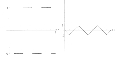
Figure 1: Graph of the five jump critical point $u_{5}$ and the derivative of the corresponding solution $v_{5}$ to (3.3).

We then compute

$$\int_{0}^{1}v_{k}^{\prime}(y)^{2}\,dy=2k\int_{0}^{\frac{1}{2k}}y^{2}\,dy=\frac{1}{3}\bigg{(}\frac{1}{2k}\bigg{)}^{2}$$

so that

$$E_{0}^{\gamma}(u_{k})=k+\frac{\gamma}{12k^{2}}.$$ (3.7)

Fixing $\gamma>0$ and minimizing over $k$, we find that the minimizer of $E_{0}^{\gamma}$ will be given by $u_{k(\gamma)}$, where $k(\gamma)$ is computable and will always be either the greatest integer less that $\bigg{(}\frac{\gamma}{6}\bigg{)}^{1/3}$ or the smallest integer bigger than $\bigg{(}\frac{\gamma}{6}\bigg{)}^{1/3}$. In particular, the number of interfaces of the minimizer is a non-decreasing function of $\gamma$ that grows like $\gamma^{1/3}.$

Alternatively, we observe that for any fixed integer $k$ the formula (3.7) is a linear function of $\gamma$ and the intersection point of any two of these lines corresponding to consecutive $k$ values moves monotonically to the right. This follows since

$$E_{0}^{\gamma}(u_{k-1})=E_{0}^{\gamma}(u_{k})\quad\mbox{implies}\quad\gamma=\gamma_{1}(k):=\frac{12k^{2}(k-1)^{2}}{2k-1}$$

while the condition

$$E_{0}^{\gamma}(u_{k})=E_{0}^{\gamma}(u_{k+1})\quad\mbox{implies}\quad\gamma=\gamma_{2}(k):=\frac{12k^{2}(k+1)^{2}}{2k+1}$$

and one readily checks that $\gamma_{1}(k)<\gamma_{2}(k)$ for every positive integer $k$. Thus, $u_{k}$ will be the minimizer for $\gamma$ lying in the interval $\gamma_{1}(k)\leqslant\gamma\leqslant\gamma_{2}(k)$. We therefore conclude:

Proposition 3.1.

For a given positive integer $k$, the $k$ interface critical points $\pm u_{k}$ will be the global minimizers of $E_{0}^{\gamma}$ on the interval

$$\frac{12k^{2}(k-1)^{2}}{2k-1}<\gamma<\frac{12k^{2}(k+1)^{2}}{2k+1}\quad\mbox{for}\quad k=1,2,\ldots$$ (3.8)

4 Two-dimensional stability of the one-dimensional critical points

Here we wish to determine the range of stability of the critical points $u_{k}$ defined in (3.5)-(3.6) with respect to the two-dimensional energy $E_{\Omega_{\varepsilon}}^{\gamma}.$ We refer the reader to [19] for an earlier derivation of stability of lamellar patterns through an entirely different approach. By stability, we mean positivity of the second variation. We recall that in a general domain $\Omega\subset\mathbb{R}^{n}$, $n$ arbitrary, the second variation of the nonlocal isoperimetric energy $E_{\Omega}^{\gamma}$ about a critical point $u\in BV(\Omega;\{\pm 1\})$ with $\Gamma:=\partial\{u=1\}\cap\Omega$ takes the form

$$\delta^{2}E_{\Omega}^{\gamma}(u;f)=\int_{\Gamma}\big{(}\left|{\nabla_{\Gamma}f}\right|^{2}-\left\|B_{\Gamma}\right\|^{2}f^{2}\big{)}\,d\mathcal{H}^{n-1}\,-\int_{\overline{\Gamma}\cap\partial\Omega}B_{\partial\Omega}(n_{\Gamma},n_{\Gamma})f^{2}\,d\mathcal{H}^{n-2}\\ +8\gamma\int_{\Gamma}\int_{\Gamma}G({\bf{x}},{\bf{\tilde{x}}})\,f({\bf{x}})\,f({\bf{\tilde{x}}})\,d\mathcal{H}^{n-1}({\bf{x}})\,d\mathcal{H}^{n-1}({\bf{\tilde{x}}})+\;4\gamma\int_{\Gamma}\nabla v\cdot n_{\Gamma}\,f^{2}\,d\mathcal{H}^{n-1}.$$ (4.1)

Here eligible functions $f$ are those lying in $H^{1}(\Gamma)$ and satisfying $\int_{\Gamma}f\,d\mathcal{H}^{n-1}=0$. The quantities $B_{\Gamma}$ and $B_{\partial\Omega}$ stand for the second fundamental form of $\Gamma$ and $\partial\Omega$, respectively, $\left\|B_{\Gamma}\right\|^{2}$ denotes the norm squared of the second fundamental form–or equivalently, the sum of the squares of the $n-1$ principal curvatures of $\Gamma$, and $G:\Omega\times\Omega\to\mathbb{R}$ denotes the Green’s function for $-\Delta$ in $\Omega$ subject to homogeneous Neumann boundary conditions. The function $v$ in the last term above denotes the solution to the Poisson equation (1.2) and $n_{\Gamma}$ denotes the outer unit normal with respect to $\{u=1\}$. We refer to [8] or [19] for details.

Let us now apply (4.1) to the setting of the previous sections by taking $\Omega=\Omega_{\varepsilon}=(0,\varepsilon)\times(0,1)$ and $u=u_{k}$ given by (3.5)-(3.6) for any positive integer $k$. Denoting by $\Gamma$ the union $\cup_{j=1}^{k}\Gamma_{j}$ of line segments $\Gamma_{j}:=(0,\varepsilon)\times\{y_{j}\}$ comprising the jump set of $u_{k}$, we evaluate $\delta^{2}E_{\Omega_{\varepsilon}}^{\gamma}(u_{k};f)$ for an arbitrary function $f\in H^{1}(\Gamma)$ satisfying

$$\int_{\Gamma}f\,d\mathcal{H}^{1}=0$$ (4.2)

to find

$$\delta^{2}E_{\Omega_{\varepsilon}}^{\gamma}(u_{k};f)=$$

$$\sum_{j=1}^{k}\int_{0}^{\varepsilon}f_{j}^{\prime}(x)^{2}\,dx+8\gamma\int_{\Gamma}\int_{\Gamma}G\,f\,f\,d\mathcal{H}^{1}\,d\mathcal{H}^{1}+4\gamma\int_{\Gamma}\bigg{(}\nabla v_{k}\cdot n_{\Gamma}\bigg{)}\,f^{2}\,d\mathcal{H}^{1}.$$ (4.3)

Here we have used the fact that ${B_{\Gamma}}\equiv 0$ and $B_{\partial\Omega}=0$ in a neighborhood of $\overline{\Gamma}\cap\partial\Omega$, and we have introduced $f_{j}$ for the restriction $f\mathrel{\vbox{\hbox to5.5pt{\vrule height=7.0pt\hfill} \hrule}}\Gamma_{j}$. It will also be convenient to introduce the notation $f_{j}=a_{j}+g_{j}$ where $a_{j}:=\fint f_{j}$ so that by (4.2) we have

$$\sum_{j=1}^{k}a_{j}=0\quad\mbox{and for each}\;j\;\mbox{we have}\quad\int_{0}^{\varepsilon}g_{j}(x)\,dx=0.$$ (4.4)

We will analyze each term of (4.3) separately. Starting with the first one, we note that by the Poincaré inequality, one has

$$\int_{0}^{\varepsilon}f_{j}^{\prime}(x)^{2}\,dx=\int_{0}^{\varepsilon}g_{j}^{\prime}(x)^{2}\,dx\geqslant\bigg{(}\frac{\pi}{\varepsilon}\bigg{)}^{2}\int_{0}^{\varepsilon}g_{j}(x)^{2}\,dx.$$ (4.5)

Next, to analyze the term involving the Green’s function we need a bit more notation. Let $\bar{f}:\Gamma\to\mathbb{R}$ denote the function given by $\bar{f}\mathrel{\vbox{\hbox to5.5pt{\vrule height=7.0pt\hfill} \hrule}}\Gamma_{j}=a_{j}$ and let $g:\Gamma\to\mathbb{R}$ be the function given by $g\mathrel{\vbox{\hbox to5.5pt{\vrule height=7.0pt\hfill} \hrule}}\Gamma_{j}=g_{j}$. Also, we introduce the measures $\mu_{\bar{f}}$ and $\mu_{g}$ via the formulas

$$\mu_{\bar{f}}=\sum_{j=1}^{k}a_{j}\delta_{\Gamma_{j}},\qquad\mu_{g}=\sum_{j=1}^{k}g_{j}\delta_{\Gamma_{j}}$$

and let $v_{\bar{f}}$ and $v_{g}$ denote the weak $H^{1}$ solutions to the Poisson equations

$$-\Delta v_{\bar{f}}=\mu_{\bar{f}},\qquad-\Delta v_{g}=\mu_{g}\quad\mbox{in}\;\Omega_{\varepsilon}$$

subject to homogeneous Neumann boundary conditions and zero mean.

Note that $v_{\bar{f}}$ will depend only on $y$ so that

$$\int_{\Gamma}\int_{\Gamma}G\,\bar{f}\,g\,d\mathcal{H}^{1}\,d\mathcal{H}^{1}=\int_{\Omega_{\varepsilon}}\int_{\Omega_{\varepsilon}}G\,d\mu_{\bar{f}}\,d\mu_{g}=\int_{\Omega_{\varepsilon}}v_{\bar{f}}\,d\mu_{g}$$

$$=\sum_{j=1}^{k}\int_{0}^{\varepsilon}\bigg{(}v_{\bar{f}}\mathrel{\vbox{\hbox to5.5pt{\vrule height=7.0pt\hfill} \hrule}}\Gamma_{j}\bigg{)}\,g_{j}(x)\,dx=\sum_{j=1}^{k}\bigg{(}v_{\bar{f}}\mathrel{\vbox{\hbox to5.5pt{\vrule height=7.0pt\hfill} \hrule}}\Gamma_{j}\bigg{)}\,\int_{0}^{\varepsilon}g_{j}(x)\,dx=0$$ (4.6)

by (4.4). Therefore, we find that

$$\int_{\Gamma}\int_{\Gamma}G\,f\,f\,d\mathcal{H}^{1}\,d\mathcal{H}^{1}=\int_{\Gamma}\int_{\Gamma}G\,(\bar{f}+g)(\bar{f}+g)\,d\mathcal{H}^{1}\,d\mathcal{H}^{1}=\int_{\Gamma}\int_{\Gamma}G\,\bar{f}\,\bar{f}\,d\mathcal{H}^{1}\,d\mathcal{H}^{1}+\int_{\Gamma}\int_{\Gamma}G\,g\,g\,d\mathcal{H}^{1}\,d\mathcal{H}^{1}$$

$$=\int_{\Omega_{\varepsilon}}\int_{\Omega_{\varepsilon}}G\,d\mu_{\bar{f}}\,d\mu_{\bar{f}}+\int_{\Omega_{\varepsilon}}\int_{\Omega_{\varepsilon}}G\,d\mu_{g}\,d\mu_{g}=\int_{\Omega_{\varepsilon}}\left|{\nabla v_{\bar{f}}}\right|^{2}\,dx\,dy+\int_{\Omega_{\varepsilon}}\left|{\nabla v_{g}}\right|^{2}\,dx\,dy.$$

Now since $v_{\bar{f}}$ satisfies $-v_{\bar{f}}^{\prime\prime}=a_{1}\delta_{\{y=y_{1}\}}+\ldots+a_{k}\delta_{\{y=y_{k}\}}$ with $v_{\bar{f}}^{\prime}(0)=0=v_{\bar{f}}^{\prime}(1)$, we can integrate and use (4.4) to obtain

$$v_{\bar{f}}^{\prime}(y)=\left\{\begin{matrix}0&\mbox{for}\;0<y<y_{1}\\ -a_{1}&\mbox{for}\;y_{1}<y<y_{2}\\ -(a_{1}+a_{2})&\mbox{for}\;y_{2}<y<y_{3}\\ \cdot&\\ \cdot&\\ \cdot&\\ -(a_{1}+a_{2}+\ldots+a_{k-1})&\mbox{for}\;y_{k-1}<y<y_{k}\\ 0&\mbox{for}\;y_{k}<y<1.\end{matrix}\right.$$

This allows us to compute the value of $\int_{\Omega_{\varepsilon}}\left|{\nabla v_{\bar{f}}}\right|^{2}=\varepsilon\int_{0}^{1}(v_{\bar{f}}^{\prime})^{2}(y)\,dy$ and we find

$$\int_{\Gamma}\int_{\Gamma}G\,f\,f=\frac{\varepsilon}{k}\left[a_{1}^{2}+(a_{1}+a_{2})^{2}+\ldots+(a_{1}+a_{2}+\ldots+a_{k-1})^{2}\right]+\int_{\Omega_{\varepsilon}}\left|{\nabla v_{g}}\right|^{2}.$$ (4.7)

It remains to compute the last integral in (4.3). In view of (3.3), (3.5) and (3.6) we have the alternating pattern

$$v_{k}^{\prime}(y_{1})=-\frac{1}{2k},\;v_{k}^{\prime}(y_{2})=\frac{1}{2k},\;v_{k}^{\prime}(y_{3})=-\frac{1}{2k},\ldots$$

(cf. Figure 1). Recalling that $\nabla v_{k}\cdot n$ denotes the outer normal derivative with respect to the set $\{u_{k}=1\}$, it then follows from (4.4) that

$$\int_{\Gamma}\bigg{(}\nabla v_{k}\cdot n\bigg{)}f^{2}d\mathcal{H}^{1}=\sum_{j=1}^{k}\int_{\Gamma_{j}}\bigg{(}\nabla v_{k}\cdot n\bigg{)}\bigg{(}a_{j}+g_{j}(x)\bigg{)}^{2}\,dx$$

$$=v_{k}^{\prime}(y_{1})\int_{\Gamma_{1}}\bigg{(}a_{1}+g_{1}(x)\bigg{)}^{2}\,dx-v_{k}^{\prime}(y_{2})\int_{\Gamma_{2}}\bigg{(}a_{2}+g_{2}(x)\bigg{)}^{2}\,dx+\ldots-(-1)^{k}v_{k}^{\prime}(y_{k})\int_{\Gamma_{k}}\bigg{(}a_{k}+g_{k}(x)\bigg{)}^{2}\,dx$$

$$=\;-\frac{\varepsilon}{2k}\sum_{j=1}^{k}a_{j}^{2}\;-\frac{1}{2k}\sum_{j=1}^{k}\int_{0}^{\varepsilon}g_{j}(x)^{2}\,dx.$$ (4.8)

Combining (4.5), (4.7) and (4.8) we conclude that

$$\delta^{2}E_{\Omega_{\varepsilon}}^{\gamma}(u_{k};f)\geqslant\left(\bigg{(}\frac{\pi}{\varepsilon}\bigg{)}^{2}-\frac{2\gamma}{k}\right)\sum_{j=1}^{k}\int_{0}^{\varepsilon}g_{j}(x)^{2}\,dx+8\gamma\int_{\Omega_{\varepsilon}}\left|{\nabla v_{g}}\right|^{2}$$

$$+\bigg{(}\frac{2\gamma\varepsilon}{k}\bigg{)}\bigg{(}4\left[a_{1}^{2}+(a_{1}+a_{2})^{2}+\ldots+(a_{1}+a_{2}+\ldots+a_{k-1})^{2}\right]-\left[a_{1}^{2}+a_{2}^{2}+\ldots+a_{k}^{2}\right]\bigg{)}.$$

(4.9)

We now claim that the quadratic form arising in the last line of (4.9) is positive definite. To see this, it is convenient to change variables in this expression by introducing

$$\alpha_{1}=a_{1},\;\alpha_{2}=a_{1}+a_{2},\;\ldots,\;\alpha_{k}=a_{1}+a_{2}+\ldots+a_{k}.$$

Then rewriting the expression in terms of the $\alpha_{j}^{\prime}s$ and using (4.4) we find after a little algebra that

$$4\left[a_{1}^{2}+(a_{1}+a_{2})^{2}+\ldots+(a_{1}+a_{2}+\ldots+a_{k-1})^{2}\right]-\left[a_{1}^{2}+a_{2}^{2}+\ldots+a_{k}^{2}\right]$$

$$=4\left[\alpha_{1}^{2}+\alpha_{2}^{2}+\ldots+\alpha_{k-1}^{2}\right]-\left[\alpha_{1}^{2}+(\alpha_{2}-\alpha_{1})^{2}+\ldots+(\alpha_{k-1}-\alpha_{k-2})^{2}+\alpha_{k-1}^{2}\right]$$

$$=2\bigg{(}\alpha_{1}^{2}+\alpha_{2}^{2}+\ldots+\alpha_{k-1}^{2}+\alpha_{1}\alpha_{2}+\alpha_{2}\alpha_{3}+\ldots+\alpha_{k-2}\alpha_{k-1}\bigg{)}$$

$$=(\alpha_{1},\alpha_{2},\ldots,\alpha_{k-1})\left(\begin{array}[]{cccc}2&1&&0\\ 1&\ddots&\ddots&\\ &\ddots&\ddots&1\\ 0&&1&2\\ \end{array}\right)\left(\begin{matrix}\alpha_{1}\\ \alpha_{2}\\ \cdot\\ \cdot\\ \cdot\\ \alpha_{k-1}\end{matrix}\right)$$

$$\geqslant\bigg{\{}2+2\cos{\bigg{(}\frac{(k-1)\pi}{k}\bigg{)}}\bigg{\}}\left[\alpha_{1}^{2}+\alpha_{2}^{2}+\ldots+\alpha_{k-1}^{2}\right]$$

since the eigenvalues of this matrix are given by

$$\lambda_{j}=2+2\cos{\bigg{(}\frac{j\pi}{k}\bigg{)}}\quad\mbox{for}\;j=1,2,\ldots,k-1$$

(see e.g. [17]).

In particular, returning to (4.9) we have established

Proposition 4.1.

For any positive integer $k$, the function $u_{k}$ given by (3.5)-(3.6) is a stable critical point of the functional $E_{\Omega_{\varepsilon}}^{\gamma}$ provided

$$\varepsilon<\pi\sqrt{\frac{k}{2\gamma}}.$$ (4.10)

We note that the stability of the lamellar configurations implies that they are in fact $L^{1}$ local minimizers, as made precise by Theorem 5.1 to follow.

5 Two-dimensional minimality of one-dimensional
minimizers

In this section we prove our main result. A crucial tool will be the the recent work in [1] and [14] on stability implying local minimality for the nonlocal isoperimetric problem. Here we present an adaptation applicable to the present setting of cylindrical domains with Neumann boundary conditions.

Theorem 5.1.

Let $\Omega\subset\mathbb{R}^{n}$ be any bounded smooth domain with $n$ arbitrary and for any positive integer $\ell$ and any positive $\varepsilon$ let $\Omega^{\ell}_{\varepsilon}\subset\mathbb{R}^{\ell+n}$ be defined as $(0,\varepsilon)^{\ell}\times\Omega$. Then for any $\gamma\geqslant 0$, given any regular critical point $u\in L^{1}(\Omega^{\ell}_{\varepsilon})$ of $E^{\gamma}_{\Omega^{\ell}_{\varepsilon}}$ such that $\overline{\partial\{u=1\}\cap\Omega^{\ell}_{\varepsilon}}$ only meets the regular part of $\partial\Omega^{\ell}_{\varepsilon}$ and $\delta^{2}E^{\gamma}_{\Omega^{\ell}_{\varepsilon}}(u;f)>0$ for all nontrivial $f\in H^{1}(\partial\{u=1\}\cap\Omega^{\ell}_{\varepsilon})$ satisfying $\int f=0$ , there exist $\delta$ and $C>0$ such that

$$E^{\gamma}_{\Omega^{\ell}_{\varepsilon}}(w)\geqslant E^{\gamma}_{\Omega^{\ell}_{\varepsilon}}(u)+C\left\|u-w\right\|_{L^{1}(\Omega^{\ell}_{\varepsilon})}^{2}\quad\mbox{whenever}\quad\left\|u-w\right\|_{L^{1}(\Omega^{\ell}_{\varepsilon})}<\delta\text{ and }\int_{\Omega}w\,dx=\int_{\Omega}u\,dx\,.$$

As mentioned before, the proof of the theorem is essentially contained in [1] and [14], but a few remarks are in order. Let us recall the classical notion of quasiminimizers of the standard perimeter. We say that a set $E\subset\Omega$ of (relative) locally finite perimeter is a strong quasiminimizer in $\Omega$ with constants $\Lambda>0$ and $r>0$ if for every $F\subset\Omega$ of (relative) locally finite perimeter with $F\Delta E\subset B_{r}(x_{0})$ for some ball $B_{r}(x_{0})$ we have that

$$P_{\Omega\cap B_{r}(x_{0})}(E)\leqslant P_{\Omega\cap B_{r}(x_{0})}(F)+\Lambda|E\Delta F|\,.$$

We recall that in particular, local minimizers of the nonlocal isoperimetric problem are quasiminimizers, cf. e.g. [1, Theorem 2.8]. The following theorem follows from the well-established regularity theory for quasiminimizers of the perimeter (see for instance [14, Theorem 3.3]).

Theorem 5.2.

Assume that $\Omega$ is smooth and let $E_{h}\subset\Omega$ be a sequence of strong quasiminimizers in $\Omega$ with uniform constants $\Lambda>0$ and $r>0$ and such that

$$\chi_{E_{h}}\to\chi_{E}\quad\text{a.e. in $\Omega$ as $h\to\infty$}$$

for some set $E$ of class $C^{1,\alpha}$, $\alpha\in(0,\frac{1}{2})$, such that either $\overline{\partial E\cap\Omega}\cap\partial\Omega=\emptyset$ or $\overline{\partial E\cap\Omega}$ meets $\partial\Omega$ orthogonally. Then, for $h$ large enough $\partial E_{h}$ is of class $C^{1,\alpha}$ and

$$\partial E_{h}\to\partial E\qquad\text{in $C^{1,\alpha}$.}$$ (5.1)

The convergence in (5.1) can be restated equivalently by saying that we may find a sequence $\Phi_{h}$ of diffeomorphisms of class $C^{1,\alpha}$ from $\overline{\Omega}$ onto itself such that $\Phi_{h}(\partial E)=\partial E_{h}$ and $\|\Phi_{h}-I\|_{C^{1,\alpha}}\to 0$, where $I$ denotes the identity map.

The following corollary is an adaptation of Theorem 5.2 to the case of the cylindrical domains $\Omega^{\ell}_{\varepsilon}$ considered in Theorem 5.1. To state it, we need to introduce some notation for even extension of sets in $\Omega^{\ell}_{\varepsilon}$. Let us express any $z\in(0,\varepsilon)^{\ell}\times\Omega$ as $z=(x_{1},\dots,x_{\ell},y_{1},\dots,y_{n})$, with $(x_{1},\dots,x_{\ell})\in(0,\varepsilon)^{\ell}$ and $(y_{1},\dots,y_{n})\in\Omega$. Then given any set $E\subset\Omega^{\ell}_{\varepsilon}$ we may perform infinitely many even reflections of the characteristic function $\chi_{E}(x_{1},\dots,x_{\ell},y_{1},\dots,y_{n})$ with respect to the $x_{1},\dots,x_{\ell}$ variables, to obtain the characteristic function of a set we denote by $\tilde{E}\subset\mathbb{R}^{\ell}\times\Omega$.

Corollary 5.3.

Let $E_{h}\subset\Omega^{\ell}_{\varepsilon}$ be a sequence of strong quasiminimizers in $\Omega^{\ell}_{\varepsilon}$ with uniform constants $\Lambda>0$ and $r>0$ and such that

$$\chi_{E_{h}}\to\chi_{E}\quad\text{a.e. in $\Omega^{\ell}_{\varepsilon}$}$$

for some set $E\subset\Omega^{\ell}_{\varepsilon}$ such that $\tilde{E}$ is of class $C^{1,\alpha}(\mathbb{R}^{\ell}\times\Omega)$, $\alpha\in(0,\frac{1}{2})$, and either $\overline{\partial\tilde{E}\cap(\mathbb{R}^{\ell}\times\Omega)}\cap\partial(\mathbb{R}^{\ell}\times\Omega)=\emptyset$ or $\overline{\partial\tilde{E}\cap(\mathbb{R}^{\ell}\times\Omega)}$ meets $\partial(\mathbb{R}^{\ell}\times\Omega)$ orthogonally.

Then, for $h$ large enough $\partial E_{h}$ is of class $C^{1,\alpha}$ and $\{E_{h}\}$ satisfies (5.1).

Proof.

The point here is that the boundary $\partial\Omega^{\ell}_{\varepsilon}$ has a “singular” part. The trick is to remove these singularities by reflection. It is straightforward to check that the reflected sets $\tilde{E}_{h}$ are strong quasiminimizers with the same uniform constants $\Lambda>0$ and $r>0$, and that

$$\chi_{\tilde{E}_{h}}\to\chi_{\tilde{E}}\quad\text{a.e. in $\mathbb{R}^{\ell}\times\Omega$.}$$

The conclusion then follows by applying Theorem 5.2 with $\Omega$ replaced by $\mathbb{R}^{\ell}\times\Omega$.

∎

Proof of Theorem 5.1. As mentioned before the proof is essentially contained in [14], where the general strategy devised in [1] in the periodic setting has been adapted to the Neumann case. It consists of two main steps.

Step 1. One shows that the positive definiteness of $\delta^{2}E^{\gamma}_{\Omega^{\ell}_{\varepsilon}}(u;f)$ implies that $u$ is an isolated local minimizer with respect to small $W^{2,p}$- perturbations, for all $p$ sufficiently large, of the free-boundary $\partial\{u=1\}\cap\Omega^{\ell}_{\varepsilon}$. Precisely, for all $p$ sufficiently large one can show the existence of $\delta>0$ such that if $\Phi:\overline{\Omega}^{\ell}_{\varepsilon}\to\overline{\Omega}^{\ell}_{\varepsilon}$ is a diffeomorphism of class $W^{2,p}$ and $\int_{\Omega^{\ell}_{\varepsilon}}u\circ\Phi\,dx=\int_{\Omega^{\ell}_{\varepsilon}}u\,dx$, then

$$E^{\gamma}_{\Omega^{\ell}_{\varepsilon}}(u\circ\Phi)\geqslant E^{\gamma}_{\Omega^{\ell}_{\varepsilon}}(u)+C\left\|u-(u\circ\Phi)\right\|_{L^{1}(\Omega^{\ell}_{\varepsilon})}^{2}\quad\mbox{provided}\quad\left\|\Phi-I\right\|_{W^{2,p}(\Omega^{\ell}_{\varepsilon})}<\delta.$$

This fact follows from [14, Proposition 5.2]: indeed, due to the assumptions on $\partial\{u=1\}\cap\Omega^{\ell}_{\varepsilon}$, the argument is not affected by the presence of a “singular” part in $\partial\Omega^{\ell}_{\varepsilon}$.

Step 2. One shows that the conclusion of the previous step implies the thesis of the Theorem. This can be argued exactly as in [14, Section 6] (see also [1, Proof of Theorem 1.1]). The proof can be reproduced word for word, using Corollary 5.3 instead of [14, Theorem 3.3]. ∎

As in the previous two sections, for convenience only at this point we fix the mass constraint $m$ to be zero. We now present our main result for the nonlocal isoperimetric problem posed on the domain $\Omega_{\varepsilon}:=(0,\varepsilon)\times(0,1)$. (This corresponds to $\ell=1$ and $\Omega=(0,1)$ in the notation $\Omega^{\ell}_{\varepsilon}$ used previously in this section.)

Theorem 5.4.

For any positive integer $k$, fix $\gamma>0$ in the interval given by (3.8). Let $a$ be any positive number smaller than $\pi\sqrt{\frac{k}{2\gamma}}$. Then for all sufficiently large integers $j$, the minimizers $\pm u_{k}$ given by (3.5)-(3.6) of the one-dimensional energy $E_{0}^{\gamma}$ are also the minimizers of the two-dimensional energy $E^{\gamma}_{\Omega_{\varepsilon_{j}}}$ where $\varepsilon_{j}:=\frac{a}{j}$ and are the only minimizers of this energy.

A typical minimizer is depicted in Figure 2. The proof consists of a combination of the $\Gamma$-convergence of Section 2, the one-dimensional minimality of $u_{k}$ established in Section 3, the two-dimensional stability shown in the previous section and Theorem 5.1.

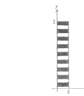
Figure 2: Graph of a typical minimizer of $E^{\gamma}_{\Omega_{\varepsilon}}$.

Proof of Theorem 5.4. Throughout the proof, $k$ and then $\gamma$ are fixed so that $u_{k}$ minimizes $E_{0}^{\gamma}.$ For any positive integer $j$, let us denote by $u_{\varepsilon_{j}}$ a global minimizer of $E^{\gamma}_{\Omega_{\varepsilon_{j}}}.$ We will argue that $u_{\varepsilon_{j}}=u_{k}$ for all large enough integers $j$.

Note first that from the choice of $a$, Proposition 4.1 guarantees that $u_{k}$ is a stable critical point of $E^{\gamma}_{\Omega_{a}}$. Applying Theorem 5.1, we can then assert the local minimality of $u_{k}$ in $\Omega_{a}$, namely the existence of a positive $\delta$ and $C$ such that

$$E^{\gamma}_{\Omega_{a}}(w)\geqslant E^{\gamma}_{\Omega_{a}}(u_{k})+C\left\|w-u_{k}\right\|_{L^{1}(\Omega_{a})}^{2}\quad\mbox{provided}\quad\left\|w-u_{k}\right\|_{L^{1}(\Omega_{a})}<\delta.$$ (5.2)

With $a$ now fixed, we apply the $\Gamma$-convergence result Theorem 2.1 to the sequence of functionals $\tilde{E}^{\gamma}_{j}:L^{1}(\Omega_{a})\to\mathbb{R}$ defined via

$$\tilde{E}^{\gamma}_{j}(\tilde{u}):=\frac{1}{\varepsilon_{j}}E^{\gamma}_{\Omega_{\varepsilon_{j}}}(u)\quad\mbox{where}\quad u(x,y):=\tilde{u}(j\,x,y)\quad\mbox{for any}\quad\tilde{u}\in L^{1}(\Omega_{a}),$$

cf. (2.2). Of course, Theorem 2.1 is phrased in terms of a sequence of rescaled nonlocal isoperimetric problems defined on the unit square $\Omega_{1}$, corresponding to $a=1$ in the present notation, but the result is unchanged if we replace $\Omega_{1}$ by $\Omega_{a}$. Since convergent sequences of minimizers have a limit which minimizes the $\Gamma$-limit $E_{0}^{\gamma}$, we conclude that the sequence $\tilde{u}_{j}:\Omega_{a}\to\mathbb{R}$ given by $\tilde{u}_{j}(x,y):=u_{\varepsilon_{j}}(x/j,y)$ which minimizes $\tilde{E}^{\gamma}_{j}$ must satisfy the condition

$$\tilde{u}_{j}\to u_{k}\;\mbox{or}\;-u_{k}\;\mbox{in}\;L^{1}(\Omega_{a})\;\mbox{as}\;j\to\infty.$$ (5.3)

The indeterminacy in (5.3) is simply due to the nonuniqueness associated with the choice of mass constraint $m=0$ since for any $u$ one has $\tilde{E}^{\gamma}_{j}(u)=\tilde{E}^{\gamma}_{j}(-u)$ and $E_{0}^{\gamma}(u)=E_{0}^{\gamma}(-u)$. Let us adopt the convention that if necessary, we multiply $\tilde{u}_{j}$ by $-1$ so as to obtain $\tilde{u}_{j}\to u_{k}$ in $L^{1}$.

Now for any integer $j>1$, we evenly reflect $j-1$ times with respect to $x$ the minimizer $u_{\varepsilon_{j}}:\Omega_{\varepsilon_{j}}\to\mathbb{R}$ to build a function defined in $\Omega_{a}$ that we denote by $u^{r}_{\varepsilon_{j}}$. If we then denote by $v_{\varepsilon_{j}}$ the solution to the Poisson problem (1.2) in $\Omega_{\varepsilon_{j}}$ with right-hand side $u_{\varepsilon_{j}}$, one readily checks that the solution to (1.2) in $\Omega_{a}$ with right-hand side $u^{r}_{\varepsilon_{j}}$ is simply given by the repeated even reflection of $v_{\varepsilon_{j}}$ as well. Note in particular that even reflection preserves the required homogeneous Neumann boundary conditions. We write $v^{r}_{\varepsilon_{j}}$ for this reflection of $v_{\varepsilon_{j}}$.

We next observe that

$$\left\|u^{r}_{\varepsilon_{j}}-u_{k}\right\|_{L^{1}(\Omega_{a})}=j\,\left\|u_{\varepsilon_{j}}-u_{k}\right\|_{L^{1}(\Omega_{\varepsilon_{j}})}=\int_{0}^{1}\int_{0}^{a}\left|{u_{\varepsilon_{j}}(x/j,y)-u_{k}}\right|\,dx\,dy=\left\|\tilde{u}_{j}-u_{k}\right\|_{L^{1}(\Omega_{a})}.$$

Invoking (5.3), we conclude that $\left\|u^{r}_{\varepsilon_{j}}-u_{k}\right\|_{L^{1}(\Omega_{a})}<\delta$ for all sufficiently large integers $j$. Consequently we may apply (5.2) with $w=u^{r}_{\varepsilon_{j}}$ to find that

$$E^{\gamma}_{\Omega_{a}}(u^{r}_{\varepsilon_{j}})\geqslant E^{\gamma}_{\Omega_{a}}(u_{k})+C\left\|u^{r}_{\varepsilon_{j}}-u_{k}\right\|_{L^{1}(\Omega_{a})}^{2}.$$ (5.4)

However, for both $u^{r}_{\varepsilon_{j}}$ and $u_{k}$ the contribution to the energy $E^{\gamma}_{\Omega_{a}}$ within each of the $j$ rectangles of width $\varepsilon_{j}$ is identical, so that

$$E^{\gamma}_{\Omega_{a}}(u^{r}_{\varepsilon_{j}})=j\,E^{\gamma}_{\Omega_{\varepsilon_{j}}}(u_{\varepsilon_{j}})\quad\mbox{and}\quad E^{\gamma}_{\Omega_{a}}(u_{k})=j\,E^{\gamma}_{\Omega_{\varepsilon_{j}}}(u_{k}).$$

By (5.4), it follows that

$$E^{\gamma}_{\Omega_{\varepsilon_{j}}}(u_{\varepsilon_{j}})\geqslant E^{\gamma}_{\Omega_{\varepsilon_{j}}}(u_{k})+\,C\,\left\|u_{\varepsilon_{j}}-u_{k}\right\|_{L^{1}(\Omega_{\varepsilon_{j}})}^{2}\quad\mbox{for all sufficiently large integers}\;j,$$

contradicting the minimality of $u_{\varepsilon_{j}}$ in $\Omega_{\varepsilon_{j}}$ unless $u_{\varepsilon_{j}}\equiv u_{k}$.∎

Remark 5.5.

The reason for the restriction in the statement of Theorem 5.4 to rectangles of width $\frac{a}{j}$ is to allow for use of the reflection argument in the proof. One could remove this restriction by strengthening Theorem 5.1, specifically by showing that under the same assumptions the conclusion holds not only for $\Omega_{\varepsilon}$ but also for $\Omega_{\eta}$ for all $\eta$ sufficiently close to $\varepsilon$ and with $\delta$ and $C$ independent of $\eta$. This could no doubt be accomplished by repeating the argument of [1] or [14], and by verifying that the minimality neighborhood is independent of $\eta$. However, we have not checked the details.

6 Generalizations to higher dimensions

We conclude with two generalizations of Theorem 5.4 applicable in higher dimensions to indicate the scope of the method. In the first, we consider $E_{\Omega_{\varepsilon}}^{\gamma}$ on a thin rectangular box in arbitrary dimension that collapses with $\varepsilon$ to a line segment. Then one can again assert that global minimizers of the one-dimensional problem remain global minimizers on sufficiently thin boxes:

Theorem 6.1.

Let $k$ and $\ell$ be any positive integers and fix $\gamma>0$ in the interval given by (3.8). Let $a$ be any positive number less than $\pi\sqrt{\frac{k}{2\gamma}}$. Then for all sufficiently large integers $j$, the minimizers $\pm u_{k}$ given by (3.5)-(3.6) of the one-dimensional energy $E_{0}^{\gamma}$ are also minimizers of the $(\ell+1)$-dimensional energy $E^{\gamma}_{\Omega^{\ell}_{\varepsilon_{j}}}$ given by (1.1) posed on the domain $\Omega^{\ell}_{\varepsilon_{j}}=(0,\varepsilon_{j})^{\ell}\times(0,1)$ where $\varepsilon_{j}:=\frac{a}{j}$. Furthermore, these are the only minimizers of this energy.

The proof of the theorem needs the following adaptation of Theorem 5.1 to the present setting.

Theorem 6.2.

Assume that for a positive integer $k$ the lamellar configuration $u_{k}$ given by (3.5)-(3.6) satisfies $\delta^{2}E^{\gamma}_{\Omega_{\varepsilon}}(u_{k};f)>0$ for all nontrivial $f\in H^{1}(\partial\{u_{k}=1\}\cap\Omega_{\varepsilon})$ satisfying $\int f=0$. Then, $u_{k}$ is an isolated local $L^{1}$-minimizer; i.e., there exist $\delta$ and $C>0$ such that

$$E^{\gamma}_{\Omega_{\varepsilon}}(w)\geqslant E^{\gamma}_{\Omega_{\varepsilon}}(u_{k})+C\left\|u_{k}-w\right\|_{L^{1}(\Omega_{\varepsilon})}^{2}\quad\mbox{whenever}\quad\left\|u_{k}-w\right\|_{L^{1}(\Omega_{\varepsilon})}<\delta\text{ and }\int_{\Omega_{\varepsilon}}w\,dx=\int_{\Omega_{\varepsilon}}u_{k}\,dx.$$

Proof of Theorem 6.2. Unlike the situation in Theorem 5.1, here $\overline{\partial\{u_{k}=1\}\cap\Omega_{\varepsilon}}$ meets also the non-regular part of $\partial\Omega_{\varepsilon}$. However, we can take advantage of the fact that we deal with a particular configuration, having flat interfaces. We denote by $\Gamma_{1}$,…, $\Gamma_{k}$ the $k$ flat interfaces of $u_{k}$. As in the first step of the proof for Theorem 5.1, one starts by deducing the isolated local minimality of $u_{k}$ with respect to configurations whose interfaces are small $W^{2,p}$-perturbations for $p$ sufficiently large, of $\Gamma_{1}$,…, $\Gamma_{k}$. To show this, one may assume that such interfaces are described by the graphs of functions $h_{i}\in W^{2,p}(\Gamma_{i})$, $i=1,\dots,k$, with $\sum_{i}\int_{\Gamma_{i}}h_{i}=0$, $\nabla h_{i}\cdot n_{\Gamma_{i}}=0$ on $\partial\Gamma_{i}$ away from corners and $\sum_{i}\|h_{i}\|_{W^{2,p}(\Gamma_{i})}$ small enough. Thus, it is possible construct a volume preserving flow $\Phi$ connecting $u_{k}$ with the perturbed configurations such that $\Phi(t,x)=x+th_{i}(\pi_{i}(x))$ in a neighborhood of $\Gamma_{i}$ for all $i=1,\dots,k$, where $\pi_{i}$ denotes the orthogonal projection on $\Gamma_{i}$. Now, one can argue exactly as in [14, Proposition 5.2], using such a flow instead of the one constructed in [14, Lemma 5.3] (see also [1, Theorem 6.2]). Once the $W^{2,p}$-minimality is established, the conclusion of the theorem follows exactly as in the second step of the proof of Theorem 5.1 (through an appeal to Corollary 5.3). ∎

Proof of Theorem 6.1. For $\ell=1$ this result reduces to Theorem 5.4. After rescaling the problem onto the unit cube in $\ell+1$ dimensions, the identity (2.2) is replaced by

$$\frac{1}{\varepsilon^{\ell}}E^{\gamma}_{\Omega^{\ell}_{\varepsilon}}(u)=\tilde{E}^{\gamma}_{\varepsilon,\ell}(\tilde{u}):=$$

$$\int_{\partial^{*}\{\tilde{u}=1\}\cap\Omega_{1}}\sqrt{\frac{1}{\varepsilon^{2}}(n_{1}^{2}+\ldots+n_{\ell}^{2})+n_{\ell+1}^{2}}\,d\mathcal{H}^{\ell}+\gamma\int_{\Omega_{1}}\left(\frac{1}{\varepsilon^{2}}(\tilde{v}_{x_{1}}^{2}+\ldots+\tilde{v}_{x_{\ell}}^{2})+\tilde{v}_{y_{1}}^{2}\right)\,dx_{1}\,\dots\,dx_{\ell}\,dy_{1}$$

where for any $u\in BV(\Omega_{\varepsilon};\{\pm 1\})$, we now denote by $\tilde{u}:\Omega_{1}\to\mathbb{R}$ the function satisfying $\tilde{u}(x_{1},\ldots,x_{\ell},y_{1})=u(\varepsilon x_{1},\ldots,\varepsilon x_{\ell},y_{1})$ with a similar definition relating the original potential $v$ associated with $u$ to the rescaled one $\tilde{v}.$ With this modification, the proof of the $\Gamma$-convergence result Theorem 2.1 proceeds without change.

Regarding the stability of the one-dimensional minimizer in higher dimensions, the statement and proof of Proposition 4.1 are unchanged in the setting where we replace $\Omega_{\varepsilon}$ by $\Omega^{\ell}_{\varepsilon}.$ Thus we again have that $u_{k}$ is stable with respect to $E^{\gamma}_{\Omega^{\ell}_{\varepsilon}}$ provided $\varepsilon<\pi\sqrt{\frac{k}{2\gamma}}$. The proof of Theorem 6.1 then proceeds as in the proof of Theorem 5.4, with the obvious alteration that the reflection of the minimizer $u_{\varepsilon_{j}}$ is carried out with respect to all the ‘thin’ variables $x_{1},x_{2},\ldots,x_{\ell}$, and using Theorem 6.2 instead of Theorem 5.1. ∎

More generally, one can take $\Omega\subset\mathbb{R}^{n}$, $n\geqslant 2$ to be an arbitrary bounded smooth domain and consider the energy $E^{\gamma}_{\Omega^{\ell}_{\varepsilon}}$ in the setting where $\Omega^{\ell}_{\varepsilon}\subset\mathbb{R}^{n+l}$ is given by $\Omega^{\ell}_{\varepsilon}:=(0,\varepsilon)^{\ell}\times\Omega$ for some positive integer $\ell$. Then one can establish the following:

Theorem 6.3.

Assume $\overline{u}:\Omega\to\mathbb{R}$ is the unique global minimizer of $E^{\gamma}_{\Omega}$ given by (1.1), with $\overline{\partial\{u=1\}\cap\Omega}\cap\partial\Omega=\emptyset$. Assume $\overline{u}$ is regular in the sense described at the beginning of Section 3 and assume furthermore that $\overline{u}$ is stable in the sense of positivity of the second variation $\delta^{2}E^{\gamma}_{\Omega}(\overline{u};f)$ given by (4.1) for all nontrivial $f\in H^{1}(\Gamma)$ satisfying $\int_{\Gamma}f\,d\mathcal{H}^{n-1}=0$ with $\Gamma:=\partial\{\overline{u}=1\}\cap\Omega$. Then there exists a positive number $a$ such that for all sufficiently large integers $j$, $\overline{u}$ is also the unique minimizer of the $(n+\ell)$-dimensional energy $E^{\gamma}_{\Omega^{\ell}_{\varepsilon_{j}}}$ where $\varepsilon_{j}:=\frac{a}{j}$.

Proof. The analog of the $\Gamma$-convergence result Theorem 2.1 requires no significant change in its proof and again Theorem 5.1 still applies here. Regarding a stability result analogous to Proposition 4.1, of course one cannot expect such an explicit determination of the critical value of $\varepsilon$ below which one has stability of $\overline{u}$ with respect to $E^{\gamma}_{\Omega^{\ell}_{\varepsilon}}$. Instead we will argue that for $\varepsilon$ small enough, the stability of $\overline{u}$ in $\Omega^{\ell}_{\varepsilon}$ follows from its assumed stability in $\Omega.$

For ease of presentation only, we will take $\ell=1$ and to simplify the notation we will write $\Omega_{\varepsilon}$ for $\Omega^{1}_{\varepsilon}$. Below we use $x$ to denote a variable in $(0,\varepsilon)$ and $y=(y_{1},\ldots,y_{n})$ to denote a variable on $\Gamma$ or in $\Omega$ as the context requires. Denoting $\Gamma_{\varepsilon}:=(0,\varepsilon)\times\Gamma$ we let $f_{\varepsilon}\in H^{1}(\Gamma_{\varepsilon})$ be any nontrivial sequence satisfying the conditions

$$\int_{\Gamma_{\varepsilon}}f_{\varepsilon}\,dx\,d\mathcal{H}^{n-1}=0\quad\mbox{and}\quad\int_{\Gamma_{\varepsilon}}f_{\varepsilon}^{2}\,dx\,d\mathcal{H}^{n-1}=\varepsilon,$$ (6.1)

where the last requirement is a convenient normalization. We wish to argue that $\delta^{2}E^{\gamma}_{\Omega_{\varepsilon}}(\overline{u};f_{\varepsilon})>0$ for all $\varepsilon$ small.

Using that $\left\|B_{\Gamma_{\varepsilon}}\right\|=\left\|B_{\Gamma}\right\|$ we see that

$$\delta^{2}E^{\gamma}_{\Omega_{\varepsilon}}(\overline{u};f_{\varepsilon})=\int_{\Gamma_{\varepsilon}}\left(\left|{\nabla_{\Gamma}f_{\varepsilon}}\right|^{2}+(\frac{\partial f_{\varepsilon}}{\partial x})^{2}\right)\,dx\,d\mathcal{H}^{n-1}-\int_{\Gamma_{\varepsilon}}\left\|B_{\Gamma}\right\|^{2}f_{\varepsilon}^{2}\,dx\,d\mathcal{H}^{n-1}$$

$$+8\gamma\int_{\Omega_{\varepsilon}}\left|{\nabla v_{f_{\varepsilon}}}\right|^{2}\,dx\,dy+4\gamma\int_{\Gamma_{\varepsilon}}\nabla\overline{v}(y)\cdot n_{\Gamma}\,f_{\varepsilon}^{2}\,dx\,d\mathcal{H}^{n-1}.$$

Here $\overline{v}$ solves the Poisson equation with right-hand side $\overline{u}$ and we adapt the approach of Section 4 in writing the Green’s function term using the solution $v_{f_{\varepsilon}}$ to the Poisson equation

$$-\Delta v_{f_{\varepsilon}}=f_{\varepsilon}\,\delta_{\Gamma_{\varepsilon}}\quad\mbox{in}\;\Omega_{\varepsilon},\quad\nabla v_{f_{\varepsilon}}\cdot n_{\partial\Omega_{\varepsilon}}=0\;\mbox{on}\;\partial\Omega_{\varepsilon}.$$ (6.2)

Then changing variables by introducing $x_{1}=\frac{x}{\varepsilon}$ and setting $\tilde{f}_{\varepsilon}(x_{1},y)=f_{\varepsilon}(\varepsilon x_{1},y)$ and $\tilde{v}_{\tilde{f}_{\varepsilon}}(x_{1},y)=v_{f_{\varepsilon}}(\varepsilon x_{1},y)$ we easily calculate that

$$\frac{1}{\varepsilon}\delta^{2}E^{\gamma}_{\Omega_{\varepsilon}}(\overline{u};f_{\varepsilon})=\delta^{2}\tilde{E}^{\gamma}_{\varepsilon}(\overline{u};\tilde{f}_{\varepsilon}):=$$

$$\int_{\Gamma_{1}}\left(\left|{\nabla_{\Gamma}\tilde{f}_{\varepsilon}}\right|^{2}+\frac{1}{\varepsilon^{2}}(\frac{\partial\tilde{f}_{\varepsilon}}{\partial x_{1}})^{2}\right)\,dx_{1}\,d\mathcal{H}^{n-1}-\int_{\Gamma_{1}}\left\|B_{\Gamma}\right\|^{2}\tilde{f}_{\varepsilon}^{2}\,dx_{1}\,d\mathcal{H}^{n-1}$$

$$+8\gamma\int_{\Omega_{1}}\left(\left|{\nabla_{y}\,\tilde{v}_{\tilde{f}_{\varepsilon}}}\right|^{2}+\frac{1}{\varepsilon^{2}}(\frac{\partial\tilde{v}_{\tilde{f}_{\varepsilon}}}{\partial x_{1}})^{2}\right)\,dx_{1}\,dy+4\gamma\int_{\Gamma_{1}}\nabla\overline{v}(y)\cdot n_{\Gamma}\,\tilde{f}_{\varepsilon}^{2}\,dx_{1}\,d\mathcal{H}^{n-1}.$$ (6.3)

Also we note that (6.1) transforms to the conditions

$$\int_{\Gamma_{1}}\tilde{f}_{\varepsilon}\,d\mathcal{H}^{n}=0,\quad\mbox{and}\quad\int_{\Gamma_{1}}\tilde{f}_{\varepsilon}^{2}\,d\mathcal{H}^{n}=1.$$ (6.4)

Now we may assume $\liminf_{\varepsilon\to 0}\delta^{2}\tilde{E}^{\gamma}_{\varepsilon}(\overline{u};\tilde{f}_{\varepsilon})<\infty$ or else we are done. Such a bound implies uniform bounds along a subsequence $\{\tilde{f}_{\varepsilon_{i}}\}$ of the form

$$\int_{\Gamma_{1}}\left|{\nabla_{\Gamma}\tilde{f}_{\varepsilon_{i}}}\right|^{2}\,dx_{1}\,d\mathcal{H}^{n-1}<C,\qquad\int_{\Gamma_{1}}\big{(}\frac{\partial\tilde{f}_{\varepsilon_{i}}}{\partial x_{1}}\big{)}^{2}\,dx_{1}\,d\mathcal{H}^{n-1}<C\varepsilon_{i}^{2}.$$

These bounds and (6.4) in turn lead to the following convergences along a further subsequence (with subsequential notation suppressed):

$$\tilde{f}_{\varepsilon_{i}}\rightharpoonup f_{0}\;\mbox{in}\;H^{1}(\Gamma_{1}),\quad\tilde{f}_{\varepsilon_{i}}\to f_{0}\;\mbox{in}\;L^{2}(\Gamma_{1})\quad\mbox{for some}\;f_{0}\in H^{1}(\Gamma_{1})$$ (6.5)

$$\mbox{such that}\quad\int_{\Gamma_{1}}f_{0}\,dx_{1}\,d\mathcal{H}^{n-1}=0,\quad\int_{\Gamma_{1}}f_{0}^{2}\,dx_{1}\,d\mathcal{H}^{n-1}=1,\quad\mbox{and}\quad f_{0}=f_{0}(y)\;\mbox{only}.$$

Applying (6.5) and the fact that $f_{0}$ is independent of $x_{1}$ to the first, second and fourth integrals in (6.3) we conclude that

$$\liminf_{\varepsilon_{i}\to 0}\int_{\Gamma_{1}}\left(\left|{\nabla_{\Gamma}\tilde{f}_{\varepsilon_{i}}}\right|^{2}+\frac{1}{\varepsilon_{i}^{2}}(\frac{\partial\tilde{f}_{\varepsilon_{i}}}{\partial x_{1}})^{2}\right)\,dx_{1}\,d\mathcal{H}^{n-1}-\int_{\Gamma_{1}}\left\|B_{\Gamma}\right\|^{2}\tilde{f}_{\varepsilon_{i}}^{2}\,dx_{1}\,d\mathcal{H}^{n-1}$$

$$+4\gamma\int_{\Gamma_{1}}\nabla\overline{v}(y)\cdot n_{\Gamma}\,\tilde{f}_{\varepsilon_{i}}^{2}\,dx_{1}\,d\mathcal{H}^{n-1}$$

$$\geqslant\int_{\Gamma_{1}}\left|{\nabla_{\Gamma}f_{0}}\right|^{2}\,dx_{1}\,d\mathcal{H}^{n-1}-\int_{\Gamma_{1}}\left\|B_{\Gamma}\right\|^{2}f_{0}^{2}\,dx_{1}\,d\mathcal{H}^{n-1}+4\gamma\int_{\Gamma_{1}}\nabla\overline{v}(y)\cdot n_{\Gamma}\,f_{0}^{2}\,dx_{1}\,d\mathcal{H}^{n-1}$$

$$=\int_{\Gamma}\left|{\nabla_{\Gamma}f_{0}}\right|^{2}\,d\mathcal{H}^{n-1}-\int_{\Gamma}\left\|B_{\Gamma}\right\|^{2}f_{0}^{2}\,d\mathcal{H}^{n-1}+4\gamma\int_{\Gamma}\nabla\overline{v}(y)\cdot n_{\Gamma}\,f_{0}^{2}\,d\mathcal{H}^{n-1}.$$ (6.6)

It remains to handle the third integral of (6.3). To this end, we note that uniform bounds on the sequence $\{\tilde{v}_{\tilde{f}_{\varepsilon_{i}}}\}$ follow as did the ones for $\{\tilde{f}_{\varepsilon_{i}}\}$ so that (after passing to a subsequence) one finds

$$\tilde{v}_{\tilde{f}_{\varepsilon_{i}}}\rightharpoonup w\;\mbox{in}\;H^{1}(\Omega_{1})\quad\mbox{and}\quad\tilde{v}_{\tilde{f}_{\varepsilon_{i}}}\to w\;\mbox{in}\;L^{2}(\Omega_{1})\quad\mbox{for some}\;w\in H^{1}(\Omega_{1})$$ (6.7)

satisfying $w=w(y)$ only and $\int_{\Omega}w\,dy=0.$ It follows that for the third integral in (6.3) one has

$$\liminf_{\varepsilon_{i}\to 0}\int_{\Omega_{1}}\left(\left|{\nabla_{y}\,\tilde{v}_{\tilde{f}_{\varepsilon_{i}}}}\right|^{2}+\frac{1}{{\varepsilon_{i}}^{2}}(\frac{\partial\tilde{v}_{\tilde{f}_{\varepsilon_{i}}}}{\partial x_{1}})^{2}\right)\,dx_{1}\,dy\geqslant\int_{\Omega}\left|{\nabla w}\right|^{2}\,dy.$$ (6.8)

As a last step in establishing the stability of $\overline{u}$ in $\Omega_{\varepsilon}$ we must identify $w$ as the solution to the Poisson problem

$$-\Delta w=f_{0}\,\delta_{\Gamma},\qquad\nabla w\cdot n_{\partial\Omega}=0\;\mbox{on}\;\partial\Omega.$$ (6.9)

To see this we note from (6.2) that $\tilde{v}_{\tilde{f}_{\varepsilon}}$ satisfies the equation

$$-\Delta_{y}\tilde{v}_{\tilde{f}_{\varepsilon}}-\frac{1}{\varepsilon^{2}}\frac{\partial^{2}\tilde{v}_{\tilde{f}_{\varepsilon}}}{\partial x_{1}^{2}}=\tilde{f}_{\varepsilon}\,\delta_{\Gamma_{1}}\quad\mbox{in}\;\Omega_{1},\quad\nabla\tilde{v}_{f_{\varepsilon}}\cdot n_{\partial\Omega_{1}}=0\;\mbox{on}\;\partial\Omega_{1}.$$

Multiplication by a test function $\phi\in C^{\infty}\big{(}\overline{\Omega}\big{)}$ (independent of $x_{1}$) and integration by parts then leads to

$$\int_{\Omega_{1}}\nabla_{y}\tilde{v}_{f_{\varepsilon}}\cdot\nabla\phi\,dx_{1}\,dy=\int_{\Gamma_{1}}\tilde{f}_{\varepsilon}\phi\,dx_{1}\,dy.$$

Applying (6.5) and (6.7) and passing to the limit as $\varepsilon_{i}\to 0$ we obtain that $w$ indeed solves (6.9). Combining (6.6) and (6.8) we conclude that

$$\liminf_{\varepsilon\to 0}\delta^{2}\tilde{E}^{\gamma}_{\varepsilon}(\overline{u};\tilde{f}_{\varepsilon})\geqslant\delta^{2}E^{\gamma}_{\Omega}(\overline{u};f_{0})>0$$

by invoking the assumed stability of $\overline{u}$ as a critical point of $E^{\gamma}_{\Omega}$. Hence, $\overline{u}$ remains stable in the thin domain $\Omega_{\varepsilon}$ as well.

The rest of the proof now follows as in the proof of Theorem 5.4, through an appeal to Theorem 5.1 and the reflection argument used before.∎

Remark 6.4.

The assumption $\overline{\partial\{u=1\}\cap\Omega}\cap\partial\Omega=\emptyset$ is certainly restrictive. It could be removed if one could extend Theorem 5.1 to the case where $\overline{\partial\{u=1\}\cap\Omega_{\varepsilon}}$ also meets the non-regular part of $\partial\Omega_{\varepsilon}$. Such an extension, which is very likely possible, would however require one to modify some of the arguments presented in [14]. As this goes beyond the purposes of the present paper, we decided to state the previous theorem under more restrictive assumptions just to illustrate the scope of the method.

Acknowledgments. The research of M.M. was supported by the ERC grant 207573 “Vectorial Problems.” The research of P.S.was supported by NSF grant DMS-1101290.

References

[1] E. Acerbi, N. Fusco and M. Morini, Minimality via second variation for a
nonlocal isoperimetric problem, Comm. Math. Phys., 322, 515-557, (2013).
[2] A. Aksimentiev, M. Fialkowski and R. Holyst,
Morphology of surfaces in mesoscopic polymers, surfactants,
electrons, or reaction-diffusion systems: methods, simulations, and
measurements, Advances in Chemical Physics, 121, 141 - 239,
(2002).
[3] G. Alberti, R. Choksi and F. Otto, Uniform energy distribution for an isoperimetric
problem with long range interactions, J. Amer. Math. Soc., 22, no. 2, 569-605, (2009).
[5] M. Bonacini and R. Cristoferi, Local and global minimality results for a nonlocal isoperimetric problem on
, Preprint (2013).
[6] R. Choksi and M. Peletier, Small volume fraction limit of the diblock copolymer
problem: I. Sharp interface functional, SIAM J. Math. Anal., 42, no. 3, 1334-1370, (2010).
[7] R. Choksi and X. Ren, On a derivation of a density functional
theory for microphase separation of diblock copolymers, Journal of
Statistical Physics, 113, 151 - 176, (2003).
[8] R. Choksi and P. Sternberg, On the first and second variations of
a nonlocal isoperimetric problem, J. Reine Angew. Math., 611, 75-108, (2008).
[9] M. Cicalese and E. Spadaro, Droplet minimizers of an isoperimetric problem with long-range interactions, C.P.A.M., 66, no. 28, 1298-1333, (2013).
[10] Y. van Gennip and M.A. Peletier, Stability of monolayers and bilayers in a copolymer-homopolymer blend model, Interfaces and Free Boundaries,
11, no. 3, 331-373, (2009).
[11] D. Goldman, C. Muratov and S. Serfaty, The -limit of the two-dimensional Ohta-Kawasaki energy. I. Droplet density,
Arch. Rat. Mech. Anal., 210, 581-613, (2013).
[12] E. Giusti, Minimal surfaces and functions of
bounded variation, Birkhäuser, 1985.
[13] V. Julin, Isoperimetric problem with coulombic repulsive term, to appear in I.U.M.J.
[14] V. Julin and G. Pisante, Minimality via second variation for microphase
separation of diblock copolymer melts, preprint, (2013). Available at http://arxiv.org/abs/1301.7213.
[15] H. Knuepfer and C.B. Muratov, On an isoperimetric problem with a competing
non-local term. I. The planar case, C.P.A.M., 66, 1126-1162, (2013).
[16] H. Knuepfer and C.B. Muratov, On an isoperimetric problem with a competing
non-local term. II. The general case, to appear in C.P.A.M., (2013).
[17] L. Lovász, Combinatorial Problems and Exercises, AMS Chelsea Pub. (1979).
[18] S. Müller, Singular perturbations as a selection criterion for periodic minimizing sequences,
Calc. Var., 1, 169-204 (1993).
[19] C. Muratov, Theory of domain patterns in systems with long-range interactions of Coulomb type, Phys. Rev. E, 66, no. 6, 066108, (2002).
[20] C. Muratov, Droplet phases in nonlocal Ginzburg-Landau models with Coulomb repulsion in two dimensions, Comm. Math. Phys., 299, no. 1, 45-87, (2010).
[21] T. Ohta and K. Kawasaki, Equilibrium morphology of block copolymer melts,
Macromolecules, 19, 2621-2632, (1986).
[22] M.A. Peletier and M. Veneroni, Stripe patterns in a model for block-copolymers, Math. Models Methods Appl. Sci., 20, no. 6, 843-907, (2010).
[23] X. Ren and L. Truskinovski, Finite scale microstructures in 1D elasticity, Journal of Elasticity, 59, No. 1-3 (2000), 319-355.
[24] X. Ren and J. Wei, On the multiplicity of two nonlocal variational problems,
SIAM J. Math. Anal., 31-4, 909-924, (2000).
[25] X. Ren and J. Wei, On the spectra of 3D lamellar solutions of the diblock copolymer problem, SIAM Math. Anal., 35, no. 1, 1-32, (2003).
[26] X. Ren and J. Wei, Spherical solutions to a nonlocal free boundary problem from diblock copolymer morphology, SIAM J. Math. Anal., 39, no. 5, 1497-1535, (2008).
[27] X. Ren and J. Wei, A double bubble in a ternary system with inhibitory long range interaction, Arch. Rat. Mech. Anal., 208, no. 1, 201-253, (2013).
[28] E. Spadaro, Uniform energy and density distribution: diblock copolymers functional, Interfaces and Free Boundaries, 11, 447-474, (2009).
[29] P. Sternberg and I. Topaloglu, On the global minimizers of a nonlocal isoperimetric
problem in two dimensions, Interfaces and Free Boundaries, 13, 155-169, (2011).
[30] I. Topaloglu, On a nonlocal isoperimetric problem on the two-sphere, Comm. Pure Appl. Anal.,
12, no. 1, 597-620, (2013)
[31] E. Thomas, D.M. Anderson, C.S. Henkee and D. Hoffman,
Periodic area-minimizing surfaces in block copolymers, Nature, 334, 598 - 601
(1988).