Probability distributions with binomial moments

Abstract.

We prove that if $p\geq 1$ and $-1\leq r\leq p-1$ then the binomial sequence $\binom{np+r}{n}$, $n=0,1,\ldots$, is positive definite and is the moment sequence of a probability measure $\nu(p,r)$, whose support is contained in $\left[0,p^{p}(p-1)^{1-p}\right]$. If $p>1$ is a rational number and $-1<r\leq p-1$ then $\nu(p,r)$ is absolutely continuous and its density function $V_{p,r}$ can be expressed in terms of the Meijer $G$-function. In particular cases $V_{p,r}$ is an elementary function. We show that for $p>1$ the measures $\nu(p,-1)$ and $\nu(p,0)$ are certain free convolution powers of the Bernoulli distribution. Finally we prove that the binomial sequence $\binom{np+r}{n}$ is positive definite if and only if either $p\geq 1$, $-1\leq r\leq p-1$ or $p\leq 0$, $p-1\leq r\leq 0$. The measures corresponding to the latter case are reflections of the former ones.

1. Introduction

This paper is devoted to binomial sequences, i.e. sequences of the form

(1) $$\left\{\binom{np+r}{n}\right\}_{n=0}^{\infty},$$

where $p,r$ are real parameters. Here the generalized binomial symbol is defined by: $\binom{a}{n}:=a(a-1)\ldots(a-n+1)/n!\,$. For example, the numbers $\binom{2n}{n}$ are moments of the arcsine law

$$\frac{1}{\pi\sqrt{x(4-x)}}\chi_{(0,4)}(x)\,dx$$

(see [2]). We are going to prove that if $p\geq 1$, $-1\leq r\leq p-1$, then the sequence (1) is positive definite and the support of the corresponding probability measure $\nu(p,r)$ is contained in the interval $[0,c(p)]$, where

(2) $$c(p):=\frac{p^{p}}{(p-1)^{p-1}}.$$

For $r=-1$ this measure has an atom at $x=0$. If in addition $p>1$ is a rational number, $-1<r\leq p-1$, then $\nu(p,r)$ is absolutely continuous and the density function $V_{p,r}$ can be expressed in terms of the Meijer $G$- (and consequently of the generalized hypergeometric) functions. In particular cases $V_{p,r}$ is an elementary function.

Similar problems were studied in [5, 6] for Raney sequences

(3) $$\left\{\binom{np+r}{n}\frac{r}{np+r}\right\}_{n=0}^{\infty}$$

(called Fuss sequences if $r=1$). It was shown that if $p\geq 1$ and $0\leq r\leq p$ then the Raney sequence (3) is positive definite and the corresponding probability measure $\mu(p,r)$ has compact support contained in $[0,c(p)]$. In particular $\mu(2,1)$ is the Marchenko-Pastur distribution, which plays an important role in the theory of random matrices, see [15, 8, 10]. Moreover, for $p>0$ we have $\mu(p,1)=\mu(2,1)^{\boxtimes p-1}$, where “$\boxtimes$” denotes the multiplicative free convolution.

The paper is organized as follows. First we study the generating function $\mathcal{D}_{p,r}$ of the sequence (1). For particular cases, namely for $p=2,3,3/2$, we express $\mathcal{D}_{p,r}$ as an elementary function. In the next part we prove that if $p\geq 1$ and $-1\leq r\leq p-1$ then the sequence is positive definite and the support of the corresponding probability measure $\nu(p,r)$ is contained in $[0,c(p)]$. If $p>1$ is rational and $-1<r\leq p-1$ then $\nu(p,r)$ can be expressed as the Mellin convolution of modified beta measures, in particular $\nu(p,r)$ is absolutely continuous, while $\nu(p,-1)$ has an atomic part at $0$. Note that the positive definiteness of the binomial sequence (1) was already proved in [5] under more restrictive assumptions (namely, that $0\leq r\leq p-1$) and the proof involved the multiplicative free and the monotonic convolution.

In the next section we study the density function $V_{p,r}$ of the absolutely continuous measures $\nu(p,r)$, where $p>1$ is rational, $-1<r\leq p-1$. We show that $V_{p,r}$ can be expressed as the Meijer $G$-function, and therefore as linear combination of the generalized hypergeometric functions. In particular we derive an elementary formula for $p=2$.

Then we concentrate on the cases $p=3$ and $p=3/2$. For particular choices of $r$ (namely, $r=0,1,2$ for $p=3$ and $r=-1/2,0,1/2$ for $r=3/2$) we express $V_{p,r}$ as an elementary function (Theorem 5.1 and Theorem 5.2).

Some of the sequences (1) have combinatorial applications and appear in the Online Encyclopedia of Integer Sequences [13] (OEIS). Perhaps the most important is $\binom{2n}{n}$ (A000984 in OEIS), the moment sequence of the arcsine distribution. The sequences $\binom{3n-1}{n}$, $\binom{3n}{n}$, $\binom{3n+1}{n}$ and $\binom{3n+2}{n}$ can be found in OEIS as A165817, A005809, A045721 and A025174 respectively. We also shed some light on sequence A091527: $\binom{3n/2-1/2}{n}4^{n}$, as well as on A061162, the even numbered terms of the former (see remarks following Theorem 5.2).

In Section 6 we study various convolution relations involving the measures $\nu(p,r)$ and $\mu(p,r)$. For example we show in Proposition 6.2 that the measures $\nu(p,-1)$ and $\nu(p,0)$ are certain free convolution powers of the Bernoulli distribution.

In Section 7 we prove that the binomial sequence (1) is positive definite if and only if either $p\geq 1$, $-1\leq r\leq p-1$ or $p\leq 0$, $p-1\leq r\leq 0$. The measures corresponding to the latter case are reflections of those corresponding to the former one. Similarly, the Raney sequence (3) is positive definite if and only if either $p\geq 1$, $0\leq r\leq p$ or $p\leq 0$, $p-1\leq r\leq 0$ or else $r=0$ (the case $r=0$ the corresponds to $\delta_{0}$). Quite surprisingly, the proof involves the monotonic convolution introduced by Muraki [7].

Finally, we provide graphical representation for selected functions $V_{p,r}$.

2. Generating functions

In this part we are going to study the generating function

(4) $$\mathcal{D}_{p,r}(z):=\sum_{n=0}^{\infty}\binom{np+r}{n}z^{n}$$

(convergent in some neighborhood of $0$) of the binomial sequence (1). First we observe relations between the functions $\mathcal{D}_{p,-1}$, $\mathcal{D}_{p,0}$ and $\mathcal{D}_{p,p-1}$.

Proposition 2.1.

For every $p\in\mathbb{R}$ we have

(5) $$\mathcal{D}_{p,-1}(z)=\frac{1}{p}+\frac{p-1}{p}\mathcal{D}_{p,0}(z)$$

and

(6) $$\mathcal{D}_{p,p-1}(z)=\frac{\mathcal{D}_{p,0}(z)-1}{pz}.$$

Proof.

These formulas are consequences of the following elementary identities:

(7) $$\frac{1}{p-1}\binom{(n+1)p-1}{n+1}=\frac{1}{p}\binom{(n+1)p}{n+1}=\binom{np+p-1}{n},$$

valid for $p\in\mathbb{R}$, $n=0,1,2,\ldots$. ∎

It turns out that $\mathcal{D}_{p,r}$ is related to the generating function

(8) $$\mathcal{B}_{p}(z):=\sum_{n=0}^{\infty}\binom{np+1}{n}\frac{z^{n}}{np+1}$$

of the Fuss numbers. This function satisfies equation

(9) $$\mathcal{B}_{p}(z)=1+z\cdot\mathcal{B}_{p}(z)^{p},$$

with the initial value $\mathcal{B}_{p}(0)=1$ (5.59 in [3]), and Lambert’s formula

(10) $$\mathcal{B}_{p}(z)^{r}=\sum_{n=0}^{\infty}\binom{np+r}{n}\frac{r\cdot z^{n}}{np+r}.$$

Since

(11) $$\mathcal{D}_{p,r}(z)=\frac{\mathcal{B}_{p}(z)^{1+r}}{p-(p-1)\mathcal{B}_{p}(z)}$$

(5.61 in [3]), it is sufficient to study the functions $\mathcal{B}_{p}$.

The simplest cases for $\mathcal{B}_{p}$ are:

$$\mathcal{B}_{0}(z) =1+z,$$

$$\mathcal{B}_{1}(z) =\frac{1}{1-z},$$

$$\mathcal{B}_{-1}(z) =\frac{1+\sqrt{1+4z}}{2},$$

$$\mathcal{B}_{2}(z) =\frac{2}{1+\sqrt{1-4z}},$$

$$\mathcal{B}_{1/2}(z) =\frac{2+z^{2}+z\sqrt{4+z^{2}}}{2},$$

which lead to

$$\mathcal{D}_{0,r}(z) =(1+z)^{r},$$

$$\mathcal{D}_{1,r}(z) =(1-z)^{-1-r},$$

$$\mathcal{D}_{-1,r}(z) =\frac{\left(\frac{1+\sqrt{1+4z}}{2}\right)^{1+r}}{\sqrt{1+4z}},$$

$$\mathcal{D}_{2,r}(z) =\frac{\left(\frac{2}{1+\sqrt{1-4z}}\right)^{r}}{\sqrt{1-4z}},$$

$$\mathcal{D}_{1/2,r}(z) =\frac{4\left(\frac{2+z^{2}+z\sqrt{4+z^{2}}}{2}\right)^{1+r}}{4+z^{2}+z\sqrt{4+z^{2}}}.$$

These examples illustrate the following general rules:

(12) $$\mathcal{B}_{p}(z) =\mathcal{B}_{1-p}(-z)^{-1},$$

(13) $$\mathcal{D}_{p,r}(z) =\mathcal{D}_{1-p,-1-r}(-z).$$

The rest of this section is devoted to the cases $p=3$ and $p=3/2$.

2.1. The case $p=3$

First we find $\mathcal{B}_{3}$.

Proposition 2.2.

For $|z|<4/27$ we have

(14) $$\mathcal{B}_{3}(z)=\frac{3}{3\cos^{2}\alpha-\sin^{2}\alpha},$$

where $\alpha=\frac{1}{3}\arcsin\left(\sqrt{27z/4}\right)$.

Note that both the maps $u\mapsto\cos^{2}\left(\frac{1}{3}\arcsin(u)\right)$ and $u\mapsto\sin^{2}\left(\frac{1}{3}\arcsin(u)\right)$ are even, hence involve only even powers of $u$ in their Taylor expansion. Therefore the functions $u\mapsto\cos^{2}\left(\frac{1}{3}\arcsin(\sqrt{u})\right)$ and $u\mapsto\sin^{2}\left(\frac{1}{3}\arcsin(\sqrt{u})\right)$ are well defined and analytic on the disc $|u|<1$.

Proof.

First we note that

$$\binom{3n+1}{n}\frac{1}{3n+1}=\frac{(3n)!}{(2n+1)!n!}=\frac{\left(\frac{1}{3}\right)_{n}\left(\frac{2}{3}\right)_{n}\left(\frac{3}{3}\right)_{n}3^{3n}}{\left(\frac{2}{2}\right)_{n}\left(\frac{3}{2}\right)_{n}2^{2n}\cdot n!},$$

where $(a)_{n}:=a(a+1)\ldots(a+n-1)$ is the Pochhammer symbol. This implies that

$$\mathcal{B}_{3}(z)={}_{2}F_{1}\!\left(\left.\frac{1}{3},\frac{2}{3};\,\frac{3}{2}\right|\frac{27z}{4}\right).$$

Now, applying the identity

$${}_{2}F_{1}\!\left(\left.a,1-a;\,3/2\right|\sin^{2}t\right)=\frac{\sin\left((2a-1)t\right)}{(2a-1)\sin t},$$

(see 15.4.14 in [9]) with $t=3\alpha$ and $a=2/3$, we get

$$\mathcal{B}_{3}(z)=\frac{3\sin\alpha}{\sin 3\alpha}=\frac{3}{3\cos^{2}\alpha-\sin^{2}\alpha}.$$

∎

Now we can give formula for $\mathcal{D}_{3,r}$.

Corollary 2.3.

For all $r\in\mathbb{R}$ we have

(15) $$\mathcal{D}_{3,r}(z)=\left(\cfrac{3}{3\cos^{2}\alpha-\sin^{2}\alpha}\right)^{r}\frac{1}{\cos^{2}\alpha-3\sin^{2}\alpha},$$

where $\alpha=\frac{1}{3}\arcsin\left(\sqrt{27z/4}\right)$, $|z|<27/4$.

Now we observe that $\mathcal{D}_{3,r}(z)$ and $\mathcal{B}_{3}(z)^{r}$ can be also expressed as hypergeometric functions.

Proposition 2.4.

For all $r\in\mathbb{R}$ and $|z|<4/27$ we have

(16) $$\mathcal{D}_{3,r}(z) ={}_{3}F_{2}\!\left(\left.\frac{1+r}{3},\frac{2+r}{3},\frac{3+r}{3};\,\frac{1+r}{2},\frac{2+r}{2}\right|\frac{27z}{4}\right),$$

(17) $$\mathcal{B}_{3}(z)^{r} ={}_{3}F_{2}\!\left(\left.\frac{r}{3},\frac{1+r}{3},\frac{2+r}{3};\,\frac{1+r}{2},\frac{2+r}{2}\right|\frac{27z}{4}\right).$$

Proof.

It is easy to check that

$$\binom{3n+r}{n}=\frac{\left(\frac{1+r}{3}\right)_{n}\left(\frac{2+r}{3}\right)_{n}\left(\frac{3+r}{3}\right)_{n}3^{3n}}{\left(\frac{1+r}{2}\right)_{n}\left(\frac{2+r}{2}\right)_{n}2^{2n}\cdot n!}$$

and

$$\binom{3n+r}{n}\frac{r}{3n+r}=\frac{\left(\frac{r}{3}\right)_{n}\left(\frac{1+r}{3}\right)_{n}\left(\frac{2+r}{3}\right)_{n}3^{3n}}{\left(\frac{1+r}{2}\right)_{n}\left(\frac{2+r}{2}\right)_{n}2^{2n}\cdot n!},$$

which leads to the statement. ∎

As a byproduct we obtain two hypergeometric identities:

Corollary 2.5.

For $a\in\mathbb{R}$, $|u|<1$ we have

(18) $${}_{3}F_{2}\!\left(\left.a,a+\frac{1}{3},a+\frac{2}{3};\,\frac{3a}{2},\frac{3a+1}{2}\right|u\right) =\frac{\left(\cfrac{3}{3\cos^{2}\alpha-\sin^{2}\alpha}\right)^{3a-1}}{\cos^{2}\alpha-3\sin^{2}\alpha},$$

(19) $${}_{3}F_{2}\!\left(\left.a,a+\frac{1}{3},a+\frac{2}{3};\,\frac{3a+1}{2},\frac{3a+2}{2}\right|u\right) =\left(\cfrac{3}{3\cos^{2}\alpha-\sin^{2}\alpha}\right)^{3a},$$

where $\alpha=\frac{1}{3}\arcsin\sqrt{u}$.

Remark. One can check, that (18) and (19) are alternative versions of the following known formulas:

(20) $${}_{3}F_{2}\!\left(\left.a,a+\frac{1}{3},a+\frac{2}{3};\,\frac{3a}{2},\frac{3a+1}{2}\right|\frac{-27z}{4(1-z)^{3}}\right) =\frac{(1-z)^{3a}}{2z+1},$$

(21) $${}_{3}F_{2}\!\left(\left.a,a+\frac{1}{3},a+\frac{2}{3};\,\frac{3a+1}{2},\frac{3a+2}{2}\right|\frac{-27z}{4(1-z)^{3}}\right) =(1-z)^{3a}$$

(7.4.1.28 and 7.4.1.29 in [12]). Indeed, putting

$$z=\frac{-4\sin^{2}\alpha}{3\cos^{2}\alpha-\sin^{2}\alpha}$$

we have

$$1-z=\frac{3}{3\cos^{2}\alpha-\sin^{2}\alpha},$$

$$\frac{-27z}{4(1-z)^{3}}=\sin^{2}\alpha\left(3\cos^{2}\alpha-\sin^{2}\alpha\right)^{2}=\sin^{2}\ 3\alpha$$

and

$$2z+1=\frac{3\left(\cos^{2}\alpha-3\sin^{2}\alpha\right)}{3\cos^{2}\alpha-\sin^{2}\alpha}.$$

Let us mention here that the sequences $\binom{3n-1}{n}$, $\binom{3n}{n}$, $\binom{3n+1}{n}$ and $\binom{3n+2}{n}$ appear in OEIS as A165817, A005809, A045721 and A025174 respectively.

2.2. The case $p=3/2$

First we compute $\mathcal{B}_{3/2}$ in terms of hypergeometric functions.

Lemma 2.6.

$$\mathcal{B}_{3/2}(z)=\frac{1-{}_{2}F_{1}\!\left(\left.\frac{-2}{3},\frac{-1}{3};\,\frac{-1}{2}\right|\frac{27z^{2}}{4}\right)}{3z^{2}}+z\cdot{}_{2}F_{1}\!\left(\left.\frac{5}{6},\frac{7}{6};\,\frac{5}{2}\right|\frac{27z^{2}}{4}\right).$$

Proof.

If $n=2k$ then the coefficient at $z^{n}$ on the right hand side is

$$-\frac{\left(\frac{-2}{3}\right)_{k+1}\left(\frac{-1}{3}\right)_{k+1}3^{3k+3}}{3\left(\frac{-1}{2}\right)_{k+1}(k+1)!2^{2k+2}}$$

$$=\frac{-(-2)\cdot 1\cdot 4\cdot\ldots\cdot(3k-2)\cdot(-1)\cdot 2\cdot 5\cdot\ldots(3k-1)3^{k+1}}{3(-1)\cdot 1\cdot 3\cdot\ldots\cdot(2k-1)(k+1)!2^{k+1}}$$

$$=\frac{1\cdot 4\cdot\ldots\cdot(3k-2)\cdot 2\cdot 5\cdot\ldots(3k-1)3^{k}}{1\cdot 3\cdot\ldots\cdot(2k-1)(k+1)!2^{k}}$$

$$=\frac{(3k)!}{(2k)!(k+1)!}=\binom{3k+1}{2k}\frac{1}{3k+1}=\binom{3n/2+1}{n}\frac{1}{3n/2+1}.$$

Now assume that $n=2k+1$. Then

$$\binom{3n/2+1}{n}\frac{1}{3n/2+1}=\frac{(6k+3)(6k+1)(6k-1)\ldots(2k+5)}{2^{2k}(2k+1)!}=\frac{(6k+3)!!}{2^{2k}(2k+3)!!(2k+1)!}.$$

On the other hand

$$\frac{\left(\frac{5}{6}\right)_{k}\left(\frac{7}{6}\right)_{k}3^{3k}}{\left(\frac{5}{2}\right)_{k}2^{2k}k!}=\frac{5\cdot 11\cdot\ldots\cdot(6k-1)\cdot 7\cdot 13\cdot\ldots\cdot(6k+1)\cdot 3^{k}}{5\cdot 7\cdot\ldots(2k+3)2^{2k}k!2^{k}}$$

$$=\frac{(6k+3)!!}{2^{2k}(2k+3)!!(2k+1)!!2^{k}k!}.$$

Since $(2k+1)!!2^{k}k!=(2k+1)!\,$, the proof is completed. ∎

Now we find formulas for these two hypergeometric functions.

Lemma 2.7.

(22) $${}_{2}F_{1}\!\left(\left.\frac{-2}{3},\frac{-1}{3};\,\frac{-1}{2}\right|u\right) =\frac{2}{3}\cos 2\beta+\frac{1}{3}\cos 4\beta,$$

(23) $${}_{2}F_{1}\!\left(\left.\frac{5}{6},\frac{7}{6};\,\frac{5}{2}\right|u\right) =\frac{27\cos\beta\sin^{3}\beta}{\sin^{3}3\beta},$$

where $\beta=\frac{1}{3}\arcsin\left(\sqrt{u}\right)$.

Proof.

We know that ${}_{2}F_{1}\!\left(\left.a,b;\,c\right|z\right)$ is the unique function $f$ which is analytic at $z=0$, with $f(0)=1$, and satisfies the hypergeometric equation:

$$z(1-z)f^{\prime\prime}(z)+\big{[}c-(a+b+1)z\big{]}f^{\prime}(z)-abf(z)=0$$

(see [1]). Now one can check that this equation is satisfied by the right hand sides of these equations (22) and (23) for given parameters $a,b,c$. ∎

Now we are ready to express $\mathcal{B}_{3/2}$ as an elementary function.

Proposition 2.8.

For $3|z|\sqrt{3}<2$ we have

$$\mathcal{B}_{3/2}(z)=\frac{3}{\left(\sqrt{3}\cos\beta-\sin\beta\right)^{2}}$$

where $\beta=\frac{1}{3}\arcsin\left(3z\sqrt{3}/2\right)$.

Proof.

In view of the previous lemmas we have

$$\mathcal{B}_{3/2}(z)=\frac{1-\frac{2}{3}\cos 2\beta-\frac{1}{3}\cos 4\beta}{\frac{4}{9}\sin^{2}3\beta}+\frac{2\sin 3\beta}{3\sqrt{3}}\frac{27\cos\beta\sin^{3}\beta}{\sin^{3}3\beta}$$

$$=\frac{3(1-\cos 2\beta)(2+\cos 2\beta)}{2\sin^{2}3\beta}+\frac{6\sqrt{3}\cos\beta\sin^{3}\beta}{\sin^{2}3\beta}$$

$$=\frac{3\sin^{2}\beta\left(3\cos^{2}\beta+\sin^{2}\beta+2\sqrt{3}\cos\beta\sin\beta\right)}{\sin^{2}3\beta}$$

$$=\frac{3\left(\sqrt{3}\cos\beta+\sin\beta\right)^{2}}{\left(3\cos^{2}\beta-\sin^{2}\beta\right)^{2}}=\frac{3}{\left(\sqrt{3}\cos\beta-\sin\beta\right)^{2}}.$$

∎

Now we provide formula for $\mathcal{D}_{3/2,r}$.

Corollary 2.9.

For all $r\in\mathbb{R}$ and $3|z|\sqrt{3}<2$ we have

$$\mathcal{D}_{3/2,r}(z)=\left(\cfrac{3}{\left(\sqrt{3}\cos\beta-\sin\beta\right)^{2}}\right)^{r}\frac{1}{\cos\beta\left(\cos\beta-\sqrt{3}\sin\beta\right)},$$

where $\beta=\frac{1}{3}\arcsin\left(3z\sqrt{3}/2\right)$.

Note also a hypergeometric expression for $\mathcal{D}_{3/2,r}$:

Proposition 2.10.

For all $r\in\mathbb{R}$ and $3|z|\sqrt{3}<2$ we have

$$\mathcal{D}_{3/2,r}(z)={}_{3}F_{2}\!\left(\left.\frac{1+r}{3},\frac{2+r}{3},\frac{3+r}{3};\,\frac{1}{2},1+r\right|\frac{27z^{2}}{4}\right)$$

$$+\frac{z(2r+3)}{2}{}_{3}F_{2}\!\left(\left.\frac{5+2r}{6},\frac{7+2r}{6},\frac{9+2r}{6};\,\frac{3}{2},\frac{3+2r}{2}\right|\frac{27z^{2}}{4}\right).$$

Proof.

If $n=2k$ then the coefficient at $z^{n}$ on the right hand side is

$$\frac{\left(\frac{1+r}{3}\right)_{k}\left(\frac{2+r}{3}\right)_{k}\left(\frac{3+r}{3}\right)_{k}3^{3k}}{\left(\frac{1}{2}\right)_{k}\left(1+r\right)_{k}2^{2k}k!}=\frac{(1+r)(2+r)(3+r)\ldots(3k+r)}{(2k-1)!!(1+r)\ldots(k+r)2^{k}k!}$$

$$=\frac{(k+1+r)(k+2+r)\ldots(3k+r)}{(2k)!}=\binom{3k+r}{2k}.$$

If, in turn, $n=2k+1$ then the coefficient at $z^{n}$ is

$$\frac{3+2r}{2}\frac{\left(\frac{5+2r}{6}\right)_{k}\left(\frac{7+2r}{6}\right)_{k}\left(\frac{9+2r}{6}\right)_{k}3^{3k}}{\left(\frac{3}{2}\right)_{k}\left(\frac{3+2r}{2}\right)_{k}2^{2k}k!}$$

$$=\frac{3+2r}{2}\frac{(5+2r)(7+2r)(9+2r)(11+2r)\ldots(6k+3+2r)}{(2k+1)!!(3+2r)(5+2r)\ldots(2k+1+2r)2^{3k}k!}$$

$$=\frac{(2k+3+2r)(2k+5+2r)\ldots(6k+3+2r)}{(2k+1)!2^{2k+1}}$$

$$=\frac{\left(\frac{3(2k+1)}{2}+r\right)\left(\frac{3(2k+1)}{2}-1+r\right)\left(\frac{3(2k+1)}{2}-2+r\right)\ldots\left(\frac{3(2k+1)}{2}-2k+r\right)}{(2k+1)!}$$

$$=\binom{3(2k+1)/2+r}{2k+1},$$

which proves the odd case. ∎

3. Mellin convolution

In this part we are going to prove that if $p\geq 1$ and $-1\leq r\leq p-1$ then the sequence (1) is positive definite. Moreover, if $p>1$ is rational and $-1<r\leq p-1$ then the corresponding probability measure $\nu(p,r)$ is absolutely continuous and is the Mellin product of modified beta distributions, see [2].

Lemma 3.1.

If $p=k/l$, where $k,l$ are integers, $1\leq l<k$, $r>-1$ and if $mp+r+1\neq 0,-1,-2,\ldots$ then

(24) $$\binom{mp+r}{m}=\frac{1}{\sqrt{2\pi l}}\left(\frac{p}{p-1}\right)^{r+1/2}\frac{\prod_{j=1}^{k}\Gamma(\beta_{j}+m/l)}{\prod_{j=1}^{k}\Gamma(\alpha_{j}+m/l)}c(p)^{m},$$

$m=0,1,2,\ldots$, where $c(p)=p^{p}(p-1)^{1-p}$,

(27) $$\alpha_{j} =\left\{\begin{array}[]{ll}\cfrac{j}{l}&\mbox{if $1\leq j\leq l$,}\\ \cfrac{r+j-l}{k-l}&\mbox{if $l+1\leq j\leq k$,}\end{array}\right.$$

(28) $$\beta_{j} =\frac{r+j}{k},\quad\qquad{1\leq j\leq k}.$$

Writing $p=k/l$ we will tacitly assume that $k,l$ are relatively prime, although this assumption is not necessary in the sequel.

Proof.

Assuming that $mp+r+1\neq 0,-1,-2,\ldots$, we have

(29) $$\binom{mp+r}{m}=\frac{\Gamma(mp+r+1)}{\Gamma(m+1)\Gamma(mp-m+r+1)}.$$

Now we apply the Gauss’s multiplication formula:

(30) $$\Gamma(nz)=(2\pi)^{(1-n)/2}n^{nz-1/2}\prod_{i=0}^{n-1}\Gamma\left(z+\frac{i}{n}\right)$$

which gives us:

$$\Gamma(mp+r+1) =\Gamma\left(k\left(\frac{m}{l}+\frac{r+1}{k}\right)\right)=(2\pi)^{(1-k)/2}k^{mk/l+r+1/2}\prod_{j=1}^{k}\Gamma\left(\frac{m}{l}+\frac{r+j}{k}\right),$$

$$\Gamma(m+1) =\Gamma\left(l\frac{m+1}{l}\right)=(2\pi)^{(1-l)/2}l^{m+1/2}\prod_{j=1}^{l}\Gamma\left(\frac{m}{l}+\frac{j}{l}\right)$$

and

$$\Gamma(mp-m+r+1) =\Gamma\left((k-l)\left(\frac{m}{l}+\frac{r+1}{k-l}\right)\right)$$

$$=(2\pi)^{(1-k+l)/2}(k-l)^{m(k-l)/l+r+1/2}\prod_{j=l+1}^{k}\Gamma\left(\frac{m}{l}+\frac{r+j-l}{k-l}\right).$$

Applying to (29) we get (24). ∎

Similarly as in [6] we need to change the enumeration of $\alpha$’s. Note that here this modification depends not only on $k,l$ but also on $r$.

Lemma 3.2.

Suppose that $k,l$ are integers such that $1\leq l<k$ and that $-1<r\leq p-1=(k-l)/l$. For $1\leq i\leq l$ define

$$j_{i}^{\prime}:=\left\lfloor\frac{ik}{l}-r\right\rfloor,$$

where $\lfloor\cdot\rfloor$ denotes the floor function. In addition we put $j_{0}^{\prime}:=0$ and $j_{l+1}^{\prime}:=k+1$, so that

$$0=j_{0}^{\prime}<j_{1}^{\prime}<j_{2}^{\prime}<\ldots<j_{l}^{\prime}\leq k<k+1=j_{l+1}^{\prime}.$$

For $1\leq j\leq k$ define

(31) $$\widetilde{\alpha}_{j}=\left\{\begin{array}[]{ll}\cfrac{i}{l}&\mbox{ if $j=j_{i}^{\prime}$, $1\leq i\leq l$,}\\ \cfrac{r+j-i}{k-l}&\mbox{ if $j_{i}^{\prime}<j<j_{i+1}^{\prime}$.}\end{array}\right.$$

Then the sequence $\left\{\widetilde{\alpha}_{j}\right\}_{j=1}^{k}$ is a permutation of $\left\{{\alpha}_{j}\right\}_{j=1}^{k}$ and we have $\beta_{j}\leq\widetilde{\alpha}_{j}$ for all $j\leq k$.

Proof.

If $j=j_{i}^{\prime}$, $1\leq i\leq l$, then we have to prove that

$$\frac{r+j_{i}^{\prime}}{k}\leq\frac{i}{l},$$

which is equivalent to

$$j_{i}^{\prime}\leq\frac{ik}{l}-r,$$

but this is a consequence of the definition of $j_{i}^{\prime}$ and the inequality $\lfloor x\rfloor\leq x$.

Now assume that $j_{i}^{\prime}<j<j_{i+1}^{\prime}$, $0\leq i\leq k$. Then we should prove that

$$\frac{r+j}{k}\leq\frac{r+j-i}{k-l},$$

which is equivalent to

$$lr+lj-ik\geq 0.$$

Since $\lfloor x\rfloor+1>x$, we have

$$lr+lj-ik\geq lr+l(j_{i}^{\prime}+1)-ik>lr+l\left(\frac{ik}{l}-r\right)-ik=0,$$

which concludes the proof. ∎

Recall that for probability measures $\mu_{1}$, $\mu_{2}$ on the positive half-line $[0,\infty)$ the Mellin convolution (or the Mellin product) is defined by

(32) $$\left(\mu_{1}\circ\mu_{2}\right)(A):=\int_{0}^{\infty}\int_{0}^{\infty}\mathbf{1}_{A}(xy)d\mu_{1}(x)d\mu_{2}(y)$$

for every Borel set $A\subseteq[0,\infty)$. This is the distribution of the product $X_{1}\cdot X_{2}$ of two independent nonnegative random variables with $X_{i}\sim\mu_{i}$. In particular, $\mu\circ\delta_{c}$ is the dilation of $\mu$:

$$\left(\mu\circ\delta_{c}\right)(A)=\mathbf{D}_{c}\mu(A):=\mu\left(\frac{1}{c}A\right)$$

($c>0$). If $\mu$ has density $f(x)$ then $\mathbf{D}_{c}(\mu)$ has density $f(x/c)/c$.

If both the measures $\mu_{1},\mu_{2}$ have all moments

$$s_{m}(\mu_{i}):=\int_{0}^{\infty}x^{m}\,d\mu_{i}(x)$$

finite then so has $\mu_{1}\circ\mu_{2}$ and

$$s_{m}\left(\mu_{1}\circ\mu_{2}\right)=s_{m}(\mu_{1})\cdot s_{m}(\mu_{2})$$

for all $m$.

If $\mu_{1},\mu_{2}$ are absolutely continuous, with densities $f_{1},f_{2}$ respectively, then so is $\mu_{1}\circ\mu_{2}$ and its density is given by the Mellin convolution:

$$\left(f_{1}\circ f_{2}\right)(x):=\int_{0}^{\infty}f_{1}(x/y)f_{2}(y)\frac{dy}{y}.$$

Similarly as in [6] we will use the modified beta distributions (see [2]):

(33) $$\mathbf{b}(u+v,u,l):=\frac{l}{\mathrm{B}(u,v)}x^{lu-1}\left(1-x^{l}\right)^{v-1}dx,\qquad x\in[0,1],$$

where $u,v,l>0$ and $\mathrm{B}$ denotes the Euler beta function. The $n$th moment of $\mathbf{b}(u+v,u,l)$ is

$$\int x^{n}\,d\mathbf{b}(u+v,u,l)(x)=\frac{\Gamma(u+n/l)\Gamma(u+v)}{\Gamma(u+v+n/l)\Gamma(u)}.$$

We also define $\mathbf{b}(u,u,l):=\delta_{1}$ for $u,l>0$.

Now we are ready to prove

Theorem 3.3.

Suppose that $p=k/l$, where $k,l$ are integers such that $1\leq l<k$, and that $r$ is a real number, $-1<r\leq p-1$. Then there exists a unique probability measure $\nu(p,r)$ such that $\binom{mp+r}{m}$ is its moment sequence. Moreover, $\nu(p,r)$ can be represented as the following Mellin convolution:

$$\nu(p,r)=\mathbf{b}(\widetilde{\alpha}_{1},\beta_{1},l)\circ\ldots\circ\mathbf{b}(\widetilde{\alpha}_{k},\beta_{k},l)\circ\delta_{c(p)},$$

where $c(p):=p^{p}(p-1)^{1-p}$. In particular, $\nu(p,r)$ is absolutely continuous and its support is $[0,c(p)]$.

The density function of $\nu(p,r)$ will be denoted by $V_{p,r}(x)$.

Proof.

In view of Lemma 3.1 and Lemma 3.2 we can write

$$\binom{mp+r}{m}=D\prod_{j=1}^{k}\frac{\Gamma(\beta_{j}+m/l)\Gamma(\widetilde{\alpha}_{j})}{\Gamma(\widetilde{\alpha}_{j}+m/l)\Gamma(\beta_{j})}\cdot c(p)^{m}$$

for some constant $D$. Taking $m=0$ we see that $D=1$. ∎

Example. Assume that $p=2$. If $-1<r\leq 0$ then

(34) $$\nu(2,r)=\mathbf{b}\left(r+1,\frac{r+1}{2},1\right)\circ\mathbf{b}\left(1,\frac{r+2}{2},1\right)\circ\delta_{4},$$

and if $0\leq r\leq 1$ then

(35) $$\nu(2,r)=\mathbf{b}\left(1,\frac{r+1}{2},1\right)\circ\mathbf{b}\left(r+1,\frac{r+2}{2},1\right)\circ\delta_{4}.$$

Theorem 3.4.

Suppose that $p,r$ are real numbers, $p\geq 1$ and $-1\leq r\leq p-1$. Then there exists a unique probability measure $\nu(p,r)$, with support contained in $[0,c(p)]$, such that $\left\{\binom{mp+r}{m}\right\}_{m=0}^{\infty}$ is its moment sequence.

Proof.

It follows from the fact that the class of positive definite sequence is closed under pointwise limits. ∎

Recall that if $\left\{s_{n}\right\}_{n=0}^{\infty}$ is positive definite, i.e. is the moment sequence of a probability measure $\mu$ on $\mathbb{R}$, then $\left\{(-1)^{n}s_{n}\right\}_{n=0}^{\infty}$ is the moment sequence of the reflection $\widehat{\mu}$ of $\mu$: $\widehat{\mu}(X):=\mu(-X)$. For the binomial sequence we have:

(36) $$\binom{np+r}{n}(-1)^{n}=\binom{n(1-p)-1-r}{n}$$

(which in particular implies (13)), hence if the binomial sequence (1), with parameters $(p,r)$, is positive definite then it is also positive definite for parameters $(1-p,-1-r)$ and we have

(37) $$\nu(1-p,-1-r)=\widehat{\nu(p,r)}.$$

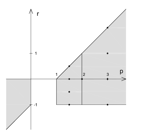
Figure 1. The set of pairs $(p,r)$ for which the binomial sequence $\binom{np+r}{n}$ is positive definite. The dots and the vertical line at $p=2$ indicate those parameters $(p,r)$ for which the density $V_{p,r}$ is an elementary function.

Therefore, if either $p\geq 1$, $-1\leq r\leq p-1$ or $p\leq 0$, $p-1\leq r\leq 0$ then the binomial sequence (1) is positive definite (for illustration see Figure 1). We will see in Theorem 7.2 that the opposite implication is also true.

Let us also note relations between the measures $\nu(p,-1)$, $\nu(p,0)$, $\nu(p,p-1)$ and observe that $\nu(p,-1)$ has an atomic part.

Proposition 3.5.

For $p\geq 1$ we have

(38) $$\nu(p,-1)=\frac{1}{p}\delta_{0}+\frac{p-1}{p}\nu(p,0)$$

and

(39) $$d\nu(p,p-1)(x)=\frac{x}{p}d\nu(p,0)(x).$$

Proof.

Both formulas follow directly from (7): for $n\geq 1$ we have

$$\binom{np-1}{n}=\frac{p-1}{p}\binom{np}{n}=\frac{p-1}{p}\int_{0}^{c(p)}x^{n}\,d\mu(p,0)(x)$$

and for $n\geq 0$

$$\binom{np+p-1}{n}=\frac{1}{p}\binom{(n+1)p}{n+1}=\frac{1}{p}\int_{0}^{c(p)}x^{n}x\,d\mu(p,0)(x).$$

∎

4. Applying Meijer $G$-function

We know already that if $p>1$ is a rational number and $-1<r\leq p-1$ then $\nu(p,r)$ is absolutely continuous. The aim of this section is to describe the density function $V_{p,r}$ of $\nu(p,r)$ in terms of the Meijer $G$-function (see [9] for example) and consequently, as a linear combination of generalized hypergeometric functions. We will see that in some particular cases $V_{p,r}$ can be represented as an elementary function.

Lemma 4.1.

For $p>1$ and $r\in\mathbb{R}$ define complex function

(40) $$\psi_{p,r}(\sigma)=\frac{\Gamma\big{(}(\sigma-1)p+r+1\big{)}}{\Gamma(\sigma)\Gamma\big{(}(\sigma-1)(p-1)+r+1\big{)}},$$

where for critical $\sigma$ the right hand side is understood as the limit if exists. Then, putting $-\mathbb{N}_{0}:=\{0,-1,-2,\ldots\}$, we have

(41) $$\psi_{p,r}(n+1)=\left\{\begin{array}[]{ll}\binom{np+r}{n}&\mbox{if }np+r+1\notin-\mathbb{N}_{0},\\ {}\\ \frac{p-1}{p}\binom{np+r}{n}&\mbox{if }np+r+1\in-\mathbb{N}_{0}.\end{array}\right.$$

Proof.

If $np+r+1\notin-\mathbb{N}_{0}$ then the statement is a consequence of the equality $\Gamma(z+1)=z\Gamma(z)$. Now recall that for the reciprocal gamma function we have

(42) $$\left.\frac{d}{dx}\frac{1}{\Gamma(x)}\right|_{x=-m}=(-1)^{m}m!,$$

for $m\in\mathbb{N}_{0}$ (see formula (3.30) in [4]). Therefore, if $np+r+1=-N$, with $N\in\mathbb{N}_{0}$, then

$$\lim_{\sigma\to n+1}\psi_{p,r}(\sigma)=\frac{(p-1)(N+n)!(-1)^{N+n}}{pn!N!(-1)^{N}}=\frac{p-1}{p}\binom{N+n}{n}(-1)^{n}$$

$$=\frac{p-1}{p}\binom{-N-1}{n}=\frac{p-1}{p}\binom{np+r}{n},$$

where we used the identity $\binom{a}{n}=\binom{n-a-1}{n}(-1)^{n}$. ∎

Note two identities which the functions $\psi_{p,r}$ satisfy:

(43) $$\psi_{p,-1}(\sigma) =\frac{p-1}{p}\psi_{p,0}(\sigma),$$

(44) $$\psi_{p,p-1}(\sigma) =\frac{1}{p}\psi_{p,0}(\sigma+1).$$

For rational $p>1$ and $r\in\mathbb{R}$ we define function $V_{p,r}(x)$ as the inverse Mellin transform of $\psi_{p,r}(\sigma)$:

(45) $$V_{p,r}(x)=\frac{1}{2\pi\mathrm{i}}\int_{d-\mathrm{i}\infty}^{d+\mathrm{i}\infty}x^{-\sigma}\psi_{p,r}(\sigma)\,d\sigma$$

whenever exists, see [14] for details. Then (43,44) imply

(46) $$V_{p,-1}(x) =\frac{p-1}{p}V_{p,0}(x),$$

(47) $$V_{p,p-1}(x) =\frac{x}{p}V_{p,0}(x).$$

It turns out that if $p>1$ is rational, $r\in\mathbb{R}$, then $V_{p,r}$ exists and can be expressed as Meijer function.

Theorem 4.2.

Let $p=k/l>1$, where $k,l$ are integers such that $1\leq l<k$, and let $r\in\mathbb{R}$. Then $V_{p,r}$ exists and can be expressed as

(48) $$V_{p,r}(x)=\frac{p^{r+1/2}\sqrt{l}}{x(p-1)^{r+1/2}\sqrt{2\pi}}\,G^{k,0}_{k,k}\!\left(\left.\!\!\begin{array}[]{ccc}\alpha_{1},\!\!&\!\!\ldots,\!\!&\!\!\alpha_{k}\\ \beta_{1},\!\!&\!\!\ldots,\!\!&\!\!\beta_{k}\end{array}\!\right|\frac{x^{l}}{c(p)^{l}}\right),$$

$x\in(0,c(p))$, where $c(p)=p^{p}(p-1)^{1-p}$ and the parameters $\alpha_{j},\beta_{j}$ are given by (27) and (28). Moreover, $\psi_{p,r}$ is the Mellin transform of $V_{p,r}$, i.e. we have

(49) $$\psi_{p,r}(\sigma)=\int_{0}^{c(p)}x^{\sigma-1}V_{p,r}(x)\,dx,$$

for $\Re\sigma>1-\frac{1+r}{p}$.

Proof.

Putting $m=\sigma-1$ in (24) we get

(50) $$\psi_{p,r}(\sigma)=\frac{(p-1)^{p-r-3/2}}{p^{p-r-1/2}\sqrt{2\pi l}}\frac{\prod_{j=1}^{k}\Gamma(\beta_{j}+\sigma/l-1/l)}{\prod_{j=1}^{k}\Gamma(\alpha_{j}+\sigma/l-1/l)}c(p)^{\sigma}.$$

Writing the right hand side as $\Psi(\sigma/l-1/l)c(p)^{\sigma}$, using the substitution $\sigma=lu+1$ and the definition of the Meijer $G$-function (see [9] for example) we obtain

$$V_{p,r}(x)=\frac{1}{2\pi\mathrm{i}}\int_{d-\mathrm{i}\infty}^{d+\mathrm{i}\infty}\Psi(\sigma/l-1/l)c(p)^{\sigma}x^{-\sigma}d\sigma=\frac{lc(p)}{2\pi x\mathrm{i}}\int_{d-\mathrm{i}\infty}^{d+\mathrm{i}\infty}\Psi(u)\left({x^{l}}/{c(p)^{l}}\right)^{-u}du$$

(51) $$=\frac{(p-1)^{p-r-3/2}\sqrt{l}}{z^{1/l}p^{p-r-1/2}\sqrt{2\pi}}G^{k,0}_{k,k}\!\left(\left.\!\!\begin{array}[]{ccc}\alpha_{1},\!\!&\!\!\ldots,\!\!&\!\!\alpha_{k}\\ \beta_{1},\!\!&\!\!\ldots,\!\!&\!\!\beta_{k}\end{array}\!\right|z\right):=\widetilde{V}_{p,r}(z),$$

$z=x^{l}/c(p)^{l}$, which leads to (48). Recall that for existence of the Meijer function of type $G^{k,0}_{k,k}$ there is no restriction on the parameters $\alpha_{j},\beta_{j}$.

On the other hand, since $\sum_{j=1}^{k}(\beta_{j}-\alpha_{j})=-1/2<0$, we can apply formula 2.24.2.1 from [12]. Substituting $x:=c(p)z^{1/l}$ we have

$$\int_{0}^{c(p)}x^{\sigma-1}V_{p,r}(x)\,dx=\frac{c(p)^{\sigma}}{l}\int_{0}^{1}z^{\sigma/l-1}\widetilde{V}_{p,r}(z)\,dz$$

$$=\frac{(p-1)^{p-r-3/2}}{p^{p-r-1/2}\sqrt{2\pi l}}c(p)^{\sigma}\int_{0}^{1}z^{\sigma/l-1/l-1}G^{k,0}_{k,k}\!\left(\left.\!\!\begin{array}[]{ccc}\alpha_{1},\!\!&\!\!\ldots,\!\!&\!\!\alpha_{k}\\ \beta_{1},\!\!&\!\!\ldots,\!\!&\!\!\beta_{k}\end{array}\!\right|z\right)\,dz=\psi_{p,r}(\sigma).$$

In view of the assumptions for the formula 2.24.2.1 in [12], the last equality holds provided $\Re(\sigma/l-1/l)>-\min_{j}\beta_{j}=-(1+r)/k$. ∎

Now we are able to describe the measures $\nu(p,r)$ for rational $p$.

Corollary 4.3.

Assume that $p=k/l$, where $k,l$ are integers, $1\leq l<k$. If $-1<r\leq p-1$ then the probability measure $\nu(p,r)$ is absolutely continuous and $V_{p,r}$ is the density function, i.e.

$$\nu(p,r)=V_{p,r}(x)\,dx,\qquad x\in(0,c(p)).$$

For $r=-1$ we have

$$\nu(p,-1)=\frac{1}{p}\delta_{0}+V_{p,-1}(x)\,dx,\qquad x\in(0,c(p)).$$

Proof.

This is a consequence of Theorem 3.3, (49), the uniqueness part of the Riesz representation theorem for linear functionals on $\mathcal{C}[0,c(p)]$ and of the Weierstrass approximation theorem. ∎

Now applying Slater’s theorem (see [4] or (16.17.2) in [9]) we can represent $V_{p,r}$ as a linear combination of generalized hypergeometric functions.

Theorem 4.4.

For $p=k/l$, with $1\leq l<k$, $r\in\mathbb{R}$ and $x\in(0,c(p))$ we have

(52) $$V_{p,r}(x)=\gamma(k,l,r)\sum_{h=1}^{k}c(h,k,l,r)\,{}_{k}F_{k-1}\!\left(\left.\begin{array}[]{c}\!\!\!\mathbf{a}(h,k,l,r)\\ \!\!\!\mathbf{b}(h,k)\end{array}\!\right|z\right)z^{(r+h)/k-1/l},$$

where $z=x^{l}/c(p)^{l}$,

(53) $$\gamma(k,l,r) =\frac{l(p-1)^{p-r-1}}{p^{p-r-1/2}\sqrt{2\pi(k-l)}},$$

(54) $$c(h,k,l,r) =\frac{\prod_{j=1}^{h-1}\Gamma\left(\frac{j-h}{k}\right)\prod_{j=h+1}^{k}\Gamma\left(\frac{j-h}{k}\right)}{\prod_{j=1}^{l}\Gamma\left(\frac{j}{l}-\frac{r+h}{k}\right)\prod_{j=l+1}^{k}\Gamma\left(\frac{r+j-l}{k-l}-\frac{r+h}{k}\right)},$$

and the parameter vectors of the hypergeometric functions are

(55) $$\mathbf{a}(h,k,l,r) =\left(\left\{\frac{r+h}{k}-\frac{j-l}{l}\right\}_{j=1}^{l},\left\{\frac{r+h}{k}-\frac{r+j-k}{k-l}\right\}_{j=l+1}^{k}\right),$$

(56) $$\mathbf{b}(h,k) =\left(\left\{\frac{k+h-j}{k}\right\}_{j=1}^{h-1},\left\{\frac{k+h-j}{k}\right\}_{j=h+1}^{k}\right).$$

Proof.

It is easy to check that if $i\neq j$ then the difference $\beta_{i}-\beta_{j}$ of coefficients (28) is not an integer and the Slater’s formula is applicable, see [9]. ∎

The easiest case is $p=2$.

Corollary 4.5.

For $p=2$, $r\in\mathbb{R}$ we have

$$V_{2,r}(x)=\frac{\cos\left(r\cdot\arccos\sqrt{x/4}\right)}{\pi\sqrt{x^{1-r}(4-x)}},$$

$x\in(0,4)$. In particular

$$V_{2,0}(x) =\frac{1}{\pi\sqrt{x(4-x)}},$$

$$V_{2,-1/2}(x) =\frac{1}{2\pi}\sqrt{\frac{\sqrt{x}+2}{\sqrt{x^{3}}(4-x)}},$$

$$V_{2,1/2}(x) =\frac{1}{2\pi}\sqrt{\frac{\sqrt{x}+2}{\sqrt{x}(4-x)}},$$

$$V_{2,1}(x) =\frac{\sqrt{x}}{2\pi\sqrt{4-x}}.$$

The density $V_{2,0}$ gives the arcsine distribution $\nu(2,0)$. Note that if $|r|>1$ then $V_{2,r}(x)<0$ for some values of $x\in(0,4)$.

Proof.

We take $k=2$, $l=1$ so that $c(2)=4$, $z=x/4$ and

$$\gamma(2,1,r)=\frac{2^{r}}{4\sqrt{\pi}}.$$

Using the Euler’s reflection formula, and the identity $\Gamma(1+r/2)=\Gamma(r/2)r/2$, we get

$$c(1,2,1,r) =\frac{\Gamma(1/2)}{\Gamma\big{(}(1-r)/2\big{)}\Gamma\big{(}(1+r)/2\big{)}}=\frac{\cos(\pi r/2)}{\sqrt{\pi}},$$

$$c(2,2,1,r) =\frac{\Gamma(-1/2)}{\Gamma(-r/2)\Gamma(r/2)}=\frac{r\sin(\pi r/2)}{\sqrt{\pi}}.$$

We also need formulas for two hypergeometric functions, namely

$${}_{2}F_{1}\!\left(\left.\frac{1+r}{2},\frac{1-r}{2};\,\frac{1}{2}\,\right|z\right) =\frac{\cos(r\arcsin\sqrt{z})}{\sqrt{1-z}},$$

$${}_{2}F_{1}\!\left(\left.\frac{2+r}{2},\frac{2-r}{2};\,\frac{3}{2}\,\right|z\right) =\frac{\sin(r\arcsin\sqrt{z})}{r\sqrt{z(1-z)}},$$

see 15.4.12 and 15.4.16 in [9]. Now we can write

$$V_{2,r}(x)=\frac{2^{r}\cos(r\pi/2)\cos(r\arcsin\sqrt{z})}{4\pi\sqrt{1-z}}z^{(r-1)/2}+\frac{2^{r}\sin(r\pi/2)\sin(r\arcsin\sqrt{z})}{4\pi\sqrt{z(1-z)}}z^{r/2}$$

$$=\frac{2^{r}z^{(r-1)/2}}{4\pi\sqrt{1-z}}\cos\left(r\pi/2-r\arcsin\sqrt{z}\right)=\frac{x^{(r-1)/2}\cos\left(r\cdot\arccos\sqrt{x/4}\right)}{\pi\sqrt{4-x}},$$

which concludes the proof of the main formula. For the particular cases we use the identity: $\cos\left(\frac{1}{2}\arccos(t)\right)=\sqrt{(t+1)/2}$. ∎

Remark. Observe that

$$\frac{V_{2,0}\left(\sqrt{x}\right)}{2\sqrt{x}}=\frac{1}{4}V_{2,-1/2}\left(\frac{x}{4}\right).$$

It means that if $X,Y$ are random variables such that $X\sim\nu(2,0)$ and $Y\sim\nu(2,-1/2)$ then $X^{2}\sim 4Y$. This can be also derived from the relation $\binom{2n-1/2}{n}4^{n}=\binom{4n}{2n}$ (sequence A001448 in OEIS).

From (38) we obtain

Corollary 4.6.

$$\nu(2,-1)=\frac{1}{2}\delta_{0}+\frac{1}{2\pi\sqrt{x(4-x)}}\chi_{(0,4)}(x)\,dx.$$

5. Some special cases for $p=3$ and $p=3/2$

From now on we are going to study some special cases for $k=3$, i.e. for $p=3$ and $p=3/2$. Then in the formula (52) we have three hypergeometric functions of type ${}_{3}F_{2}$ with lower parameters

$$\mathbf{b}(1,3)=\left(\frac{1}{3},\frac{2}{3}\right),\qquad\mathbf{b}(2,3)=\left(\frac{2}{3},\frac{4}{3}\right),\qquad\mathbf{b}(3,3)=\left(\frac{4}{3},\frac{5}{3}\right).$$

It turns out that for particular choices of $r$ these hypergeometric functions reduce to the type ${}_{2}F_{1}$, belonging to the following one-parameter family:

(57) $${}_{2}F_{1}\!\left(\left.\frac{t}{2},\frac{t+1}{2};\,t\right|z\right)=\frac{\left(1+\sqrt{1-z}\right)^{1-t}}{2^{1-t}\sqrt{1-z}}$$

(see formula 15.4.18 in [9]).

Let us start with $p=3$.

Theorem 5.1.

For $p=3$ we have

$$V_{3,0}(x) =\frac{\left(1+\sqrt{1-z}\right)^{1/3}}{9\pi\sqrt{3(1-z)}}z^{-2/3}+\frac{\left(1+\sqrt{1-z}\right)^{-1/3}}{9\pi\sqrt{3(1-z)}}z^{-1/3},$$

$$V_{3,1}(x) =\frac{\left({1+\sqrt{1-z}}\right)^{2/3}}{6\pi\sqrt{3(1-z)}}z^{-1/3}+\frac{\left({1+\sqrt{1-z}}\right)^{-2/3}}{6\pi\sqrt{3(1-z)}}z^{1/3},$$

$$V_{3,2}(x) =\frac{\left(1+\sqrt{1-z}\right)^{1/3}}{4\pi\sqrt{3(1-z)}}z^{1/3}+\frac{\left(1+\sqrt{1-z}\right)^{-1/3}}{4\pi\sqrt{3(1-z)}}z^{2/3},$$

where $z=4x/27$ and $x\in(0,27/4)$.

Proof.

We have $c(3)=27/4$ and

$$\gamma(3,1,r) =\frac{2^{1-r}}{3^{5/2-r}\sqrt{\pi}},$$

$$c(1,3,1,r) =\frac{2^{(r+1)/3}\sin\left(\pi(1+r)/3\right)}{\sqrt{3\pi}},$$

$$c(2,3,1,r) =\frac{2^{(r-1)/3}(1-r)\sin\left(\pi(1-r)/3\right)}{\sqrt{3\pi}},$$

$$c(3,3,1,r) =\frac{2^{(r-6)/3}(3-r)r\sin\left(\pi r/3\right)}{\sqrt{3\pi}}$$

and the upper parameters for the hypergeometric functions are

$$\mathbf{a}(1,3,1,r) =\left(\frac{1+r}{3},\frac{5-r}{6},\frac{2-r}{6}\right),$$

$$\mathbf{a}(2,3,1,r) =\left(\frac{2+r}{3},\frac{7-r}{6},\frac{4-r}{6}\right),$$

$$\mathbf{a}(3,3,1,r) =\left(\frac{3+r}{3},\frac{9-r}{6},\frac{6-r}{6}\right).$$

For $r=0$ we have $c(3,3,1,0)=0$ and

$$V_{3,0}(x)=\frac{2}{9\sqrt{3\pi}}\left(\frac{2^{1/3}}{2\sqrt{\pi}}\frac{\left(1+\sqrt{1-z}\right)^{1/3}}{2^{1/3}\sqrt{1-z}}z^{-2/3}+\frac{2^{-1/3}}{2\sqrt{\pi}}\frac{\left(1+\sqrt{1-z}\right)^{-1/3}}{2^{-1/3}\sqrt{1-z}}z^{-1/3}\right)$$

$$=\frac{\left(1+\sqrt{1-z}\right)^{1/3}}{9\pi\sqrt{3(1-z)}}z^{-2/3}+\frac{\left(1+\sqrt{1-z}\right)^{-1/3}}{9\pi\sqrt{3(1-z)}}z^{-1/3}.$$

For $r=1$ the second term vanishes and

$$V_{3,1}(x)=\frac{1}{3\sqrt{3\pi}}\left(\frac{2^{2/3}}{2\sqrt{\pi}}\frac{\left({1+\sqrt{1-z}}\right)^{2/3}}{2^{2/3}\sqrt{1-z}}z^{-1/3}+\frac{2^{-5/3}}{\sqrt{\pi}}\frac{\left({1+\sqrt{1-z}}\right)^{-2/3}}{2^{-2/3}\sqrt{1-z}}z^{1/3}\right)$$

$$=\frac{\left({1+\sqrt{1-z}}\right)^{2/3}}{6\pi\sqrt{3(1-z)}}z^{-1/3}+\frac{\left({1+\sqrt{1-z}}\right)^{-2/3}}{6\pi\sqrt{3(1-z)}}z^{1/3}.$$

Finally, for the third formula we can apply (39), which gives us $V_{3,2}(x)=\frac{9z}{4}V_{3,0}(x)$. ∎

Similarly we work with $p=3/2$.

Theorem 5.2.

For $p=3/2$ we have

$$V_{3/2,-1/2}(x) =\frac{\left({1+\sqrt{1-z}}\right)^{2/3}}{3\pi\sqrt{3(1-z)}}z^{-1/3}+\frac{\left({1+\sqrt{1-z}}\right)^{-2/3}}{3\pi\sqrt{3(1-z)}}z^{1/3},$$

$$V_{3/2,0}(x) =\frac{\left(1+\sqrt{1-z}\right)^{1/3}}{3\pi\sqrt{1-z}}z^{-1/6}+\frac{\left({1+\sqrt{1-z}}\right)^{-1/3}}{3\pi\sqrt{1-z}}z^{1/6},$$

$$V_{3/2,1/2}(x) =\frac{\left({1+\sqrt{1-z}}\right)^{1/3}}{\pi\sqrt{3(1-z)}}z^{1/3}+\frac{\left({1+\sqrt{1-z}}\right)^{-1/3}}{\pi\sqrt{3(1-z)}}z^{2/3},$$

where $z=4x^{2}/27$, $x\in(0,\sqrt{27/4})$.

Proof.

We have $c(3/2)=\sqrt{27}/2$,

$$\gamma(3,2,r) =\frac{2\cdot 3^{r}}{3\sqrt{\pi}},$$

$$c(1,3,2,r) =\frac{2^{(1-2r)/3}\sin\left(\pi(1-2r)/3\right)}{\sqrt{3\pi}},$$

$$c(2,3,2,r) =\frac{2^{(-1-2r)/3}(1+2r)\sin\left(\pi(1+2r)/3\right)}{\sqrt{3\pi}},$$

$$c(3,3,2,r) =\frac{2^{(-3-2r)/3}(3+2r)r\sin\left(2\pi r/3\right)}{\sqrt{3\pi}}$$

and

$$\mathbf{a}(1,3,2,r) =\left(\frac{5+2r}{6},\frac{1+r}{3},\frac{1-2r}{3}\right),$$

$$\mathbf{a}(2,3,2,r) =\left(\frac{7+2r}{6},\frac{2+r}{3},\frac{2-2r}{3}\right),$$

$$\mathbf{a}(3,3,2,r) =\left(\frac{9+2r}{6},\frac{3+r}{3},\frac{3-2r}{3}\right).$$

For $r=-1/2$ the second term vanishes and we have

$$V_{3/2,-1/2}(x)=\frac{2}{3\sqrt{3\pi}}\left(\frac{2^{2/3}}{2\sqrt{\pi}}\frac{\left({1+\sqrt{1-z}}\right)^{2/3}}{2^{2/3}\sqrt{1-z}}z^{-1/3}+\frac{2^{-2/3}}{2\sqrt{\pi}}\frac{\left({1+\sqrt{1-z}}\right)^{-2/3}}{2^{-2/3}\sqrt{1-z}}z^{1/3}\right)$$

$$=\frac{\left({1+\sqrt{1-z}}\right)^{2/3}}{3\pi\sqrt{3(1-z)}}z^{-1/3}+\frac{\left({1+\sqrt{1-z}}\right)^{-2/3}}{3\pi\sqrt{3(1-z)}}z^{1/3}.$$

For $r=0$ we note that $c(3,3,2,0)=0$ and we get

$$V_{3/2,0}(x)=\frac{2}{3\sqrt{\pi}}\left(\frac{2^{1/3}}{2\sqrt{\pi}}\frac{\left(1+\sqrt{1-z}\right)^{1/3}}{2^{1/3}\sqrt{1-z}}z^{-1/6}+\frac{2^{-1/3}}{2\sqrt{\pi}}\frac{\left(1+\sqrt{1-z}\right)^{-1/3}}{2^{-1/3}\sqrt{1-z}}z^{1/6}\right)$$

$$=\frac{\left(1+\sqrt{1-z}\right)^{1/3}}{3\pi\sqrt{1-z}}z^{-1/6}+\frac{\left({1+\sqrt{1-z}}\right)^{-1/3}}{3\pi\sqrt{1-z}}z^{1/6}.$$

Finally, by (39) we have $V_{3/2,1/2}(x)=\sqrt{3z}V_{3/2,0}(x)$, which leads to the third formula. ∎

Let us mention that the integer sequence $\binom{3n/2-1/2}{n}4^{n}$:

$$1,4,30,256,2310,21504,204204,1966080,19122246,\ldots$$

appears in OEIS as A091527. It is the moment sequence of the density function

(58) $$V(x):=V_{3/2,-1/2}(x/4)/4$$

$$=\frac{x^{4/3}+9\cdot 2^{4/3}\left(1+\sqrt{1-x^{2}/108}\right)^{4/3}}{2^{8/3}\cdot 3^{5/2}\cdot\pi\cdot x^{2/3}\sqrt{1-x^{2}/108}\left(1+\sqrt{1-x^{2}/108}\right)^{2/3}}$$

on $(0,6\sqrt{3})$ (see Theorem 5.2) and its generating function is $\mathcal{D}_{3/2,-1/2}(4z)$ (see Corollary 2.9). The even numbered terms constitute sequence A061162, i.e.

$$\mathrm{A091527}(2n)=\mathrm{A061162}(n)=\binom{3n-1/2}{2n}16^{n}=\frac{(6n)!n!}{(3n)!(2n)!^{2}},$$

so this is the moment sequence for the density function

(59) $$\frac{V\left(\sqrt{x}\right)}{2\sqrt{x}}=\frac{x^{2/3}+9\cdot 2^{4/3}\left(1+\sqrt{1-x/108}\right)^{4/3}}{2^{11/3}\cdot 3^{5/2}\cdot\pi\cdot x^{5/6}\sqrt{1-x/108}\left(1+\sqrt{1-x/108}\right)^{2/3}}$$

on the interval $(0,108)$.

From (38) we can also write down the measures $\nu(3,-1)$ and $\nu(3/2,-1)$:

$$\nu(3,-1)=\frac{1}{3}\delta_{0}+\frac{2}{3}V_{3,0}(x)\,dx,$$

$$\nu(3/2,-1)=\frac{2}{3}\delta_{0}+\frac{1}{3}V_{3/2,0}(x)\,dx.$$

6. Some convolution relations

In this part we are going to prove a few formulas involving the measures $\nu(p,r)$, the measures $\mu(p,r)$ studied in [5, 6], and various types of convolutions. First we observe that the families $\nu(p,r)$ and $\mu(p,r)$ are related through the Mellin convolution.

Proposition 6.1.

For $c>0$ define probability measure $\eta(c)$ by

$$\eta(c):=c\cdot x^{c-1}\,dx,\quad x\in[0,1].$$

Then for $p>1$, $0<r\leq p$ we have

$$\nu(p,r-1)\circ\eta\left(r/(p-1)\right)=\mu(p,r).$$

Proof.

Since the moment sequence of $\eta(c)$ is $\left\{\frac{c}{n+c}\right\}_{n=0}^{\infty}$, it is sufficient to note that

$$\binom{np+r-1}{n}\cdot\frac{r}{n(p-1)+r}=\binom{np+r}{n}\frac{r}{np+r}.$$

∎

Note that Theorem 5.1 in [5] is a consequence of Theorem 3.4 and Proposition 6.1.

For a compactly supported probability measure $\mu$ on $\mathbb{R}$ define its moment generating function by

$$M_{\mu}(z):=\int_{\mathbb{R}}\frac{1}{1-xz}\,d\mu(x).$$

For two such measures $\mu_{1},\mu_{2}$ we define their monotonic convolution (due to Muraki [7]) $\mu_{1}\vartriangleright\mu_{2}$ by

$$M_{\mu_{1}\vartriangleright\mu_{2}}(z)=M_{\mu_{1}}\big{(}zM_{\mu_{2}}(z)\big{)}\cdot M_{\mu_{2}}(z).$$

It is an associative, noncommutative operation on probability measures on $\mathbb{R}$.

Let $\mu$ be a probability measure with compact support contained in the positive halfline $[0,+\infty)$ and $\mu\neq\delta_{0}$. Then the $S$-transform, defined by

$$M_{\mu}\left(\frac{z}{1+z}S_{\mu}(z)\right)=1+z$$

can be used to describe the dilation $\mathbf{D}_{c}\mu$, the multiplicative free power $\mu^{\boxtimes p}$, the additive free power $\mu^{\boxplus t}$ and the Boolean power $\mu^{\uplus u}$ by:

(60) $$S_{\mathbf{D}_{c}\mu}(z) =\frac{1}{c}S_{\mu}(z),$$

(61) $$S_{\mu^{\boxtimes p}}(z) =S_{\mu}(z)^{p},$$

(62) $$S_{\mu^{\boxplus t}}(z) =\frac{1}{t}S_{\mu}\left(\frac{z}{t}\right),$$

(63) $$S_{\mu^{\uplus u}}(z) =\frac{1}{u}S_{\mu}\left(\frac{z}{u+(u-1)z}\right).$$

These measures are well defined (and have compact support contained in the positive half-line) for $c,u>0$ and at least for $p,t\geq 1$. The Boolean power can be also described through the moment generating function:

$$M_{\mu^{\uplus u}}(z)=\frac{M_{\mu}(z)}{u-(u-1)M_{\mu}(z)}.$$

For example, $S_{\mu(p,1)}(z)=(1+z)^{1-p}$, which implies that $\mu(p,1)=\mu(2,1)^{\boxtimes p-1}$.

Recall from [5] three formulas, which are consequences of (11) and of the identity:

$$\mathcal{B}_{p-r}\left(z\mathcal{B}_{p}(z)^{r}\right)=\mathcal{B}_{p}(z).$$

Proposition 6.2.

For $p\geq 1$, $-1\leq r\leq p-1$ and $0\leq a,b,s\leq p$ we have

(64) $$\nu(p,0)=\mu(p,1)^{\uplus p} =\left(\mu(2,1)^{\boxtimes p-1}\right)^{\uplus p},$$

(65) $$\mu(p,a)\vartriangleright\mu(p+b,b) =\mu(p+b,a+b),$$

(66) $$\nu(p,r)\vartriangleright\mu(p+s,s) =\nu(p+s,r+s).$$

In particular, if $0\leq r\leq p-1$ then

$$\nu(p,r)=\nu(p-r,0)\vartriangleright\mu(p,r)=\mu(p-r,1)^{\uplus p-r}\vartriangleright\mu(p,r).$$

The formulas (65) and (66) will be applied in the next section.

Finally we observe that $\nu(p,-1)$ and $\nu(p,0)$ are free convolutions powers of the Bernoulli distribution.

Proposition 6.3.

For $p>1$ we have

(67) $$\nu(p,-1) =\mathbf{D}_{c(p)}\left(\frac{1}{p}\delta_{0}+\frac{p-1}{p}\delta_{1}\right)^{\boxtimes p},$$

where $$c(p)=p^{p}(p-1)^{1-p}$$, and

(68) $$\nu(p,0) =\mathbf{D}_{p}\left(\left(\frac{1}{p}\delta_{0}+\frac{p-1}{p}\delta_{1}\right)^{\boxplus p/(p-1)}\right)^{\boxtimes p-1}.$$

Proof.

First we prove that

(69) $$S_{\nu(p,-1)}(z) =\frac{(p-1)^{p-1}}{p^{p}}\left(\frac{1+z}{\frac{p-1}{p}+z}\right)^{p},$$

(70) $$S_{\nu(p,0)}(z) =\frac{(p-1)^{p-1}}{p^{p}}\left(\frac{\frac{p}{p-1}+z}{1+z}\right)^{p-1}.$$

Indeed, putting $w=\frac{z}{(p-1)(1+z)}$ we have $1+w=\frac{pz+p-1}{(p-1)(1+z)}$. Therefore

$$\mathcal{D}_{p,-1}\left(w(1+w)^{-p}\right)=\frac{1}{p-(p-1)(1+w)}=1+z.$$

Similarly, putting $v=\frac{z}{p-z+pz}$ we get $1+v=\frac{p(1+z)}{p-z+pz}$ and

$$\mathcal{D}_{p,0}\left(v(1+v)^{-p}\right)=\frac{1+v}{p-(p-1)(1+v)}=1+z.$$

Now it remains to note that the $S$-transform of $\alpha\delta_{0}+(1-\alpha)\delta_{a}$, with $0<\alpha<1$, $a>0$, is $\frac{1+z}{a(1-\alpha+z)}$ and recall that $S_{\mu(2,1)}(z)=(1+z)^{-1}$. ∎

Let us note two particular cases:

(71) $$\nu(2,-1)=\mathbf{D}_{4}\left(\frac{1}{2}\delta_{0}+\frac{1}{2}\delta_{1}\right)^{\boxtimes 2}\qquad\hbox{and}\qquad\nu(2,0)=\mathbf{D}_{2}\left(\frac{1}{2}\delta_{0}+\frac{1}{2}\delta_{1}\right)^{\boxplus 2}.$$

7. The necessary conditions for positive definiteness

This section is fully devoted to the necessary conditions for the positive definiteness of the binomial (1) and Raney (3) sequences.

For the Raney sequence (3) we have

(72) $$\binom{np+r}{n}\frac{r(-1)^{n}}{np+r}=\binom{n(1-p)-r}{n}\frac{-r}{n(1-p)-r}$$

which yields (12) and

(73) $$\mu(1-p,-r)=\widehat{\mu(p,r)}.$$

Therefore, if either $p\geq 1$, $0\leq r\leq p$ or $p\leq 0$, $p-1\leq r\leq 0$ then the Raney sequence (3) is positive definite. In addition, if $r=0$ then the sequence is just $(1,0,0,\ldots)$, the moment sequence of $\delta_{0}$.

We are going to prove that these statements fully characterize positive definiteness of these sequences. We will need the following

Lemma 7.1.

Let $\left\{s_{n}\right\}_{n=0}^{\infty}$ be a sequence of real numbers and let $w:(a,b)\to\mathbb{R}$ be a continuous function, such that $w(x_{0})<0$ for some $x_{0}\in(a,b)$ and there is $N$ such that $s_{n}=\int_{a}^{b}x^{n}w(x)\,dx$ for $n\geq N$. Then $\left\{s_{n}\right\}_{n=0}^{\infty}$ is not positive definite.

Proof.

Put $w_{0}(x):=w(x)x^{2N}$ and $a_{n}:=s_{2N+n}$. Then $a_{n}:=\int_{a}^{b}w_{0}(x)x^{n}\,dx$ and in view of the the uniqueness part of the Riesz representation theorem for linear functionals on $\mathcal{C}[a,b]$ and of the Weierstrass approximation theorem, the sequence $\left\{a_{n}\right\}_{n=0}^{\infty}$ is not positive definite. Since

$$\sum_{i,j}a_{i+j}\alpha_{i}\alpha_{j}=\sum_{i,j}s_{(N+i)+(N+j)}\alpha_{i}\alpha_{j},$$

the sequence $\left\{s_{n}\right\}_{n=0}^{\infty}$ is not positive definite too. ∎

Now we are ready to prove the main result of this section. Note that formulas (65) and (66) play key role in the proof.

Theorem 7.2.

1. The binomial sequence (1) is positive definite if and only if either $p\geq 1$, $-1\leq r\leq p-1$ or $p\leq 0$, $p-1\leq r\leq 0$.

2. The Raney sequence (3) is positive definite if and only if either $p\geq 1$, $0\leq r\leq p$ or $p\leq 0$, $p-1\leq r\leq 0$ or else $r=0$.

Proof.

We need only to prove that these conditions are necessary.

First we note that the maps $(p,r)\mapsto(1-p,-1-r)$ and $(p,r)\mapsto(1-p,-r)$ are reflections with respect to the points $(1/2,-1/2)$ and $(1/2,0)$ respectively. Therefore it is sufficient to confine ourselves to $p\geq 1/2$. First we will show that if the binomial sequence (1) (resp. the Raney sequence 3) is positive definite and $p\geq 1/2$ then $p\geq 1$ (or $r=0$ in the case or Raney sequence).

We will use the fact that if a sequence $\left\{s_{n}\right\}_{n=0}^{\infty}$ is positive definite then $s_{2n}\geq 0$ and $\det\left(s_{i+j}\right)_{i,j=0}^{n}\geq 0$ for all $n\in\mathbb{N}$. Then the condition $\det\left(s_{i+j}\right)_{i,j=0}^{1}\geq 0$ is equivalent to

(74) $$2p^{2}-2p-r-r^{2} \geq 0,$$

for the binomial sequence (1) and

(75) $$r(2p-r-1) \geq 0$$

for the Raney sequence (3).

Assume that $1/2\leq p<1$, $r\in\mathbb{R}$ and that the binomial sequence (1) is positive definite. Then (74) implies that $-1\leq r\leq 0$ and $\frac{1}{2}+\frac{1}{2}\sqrt{1+r+r^{2}}\leq p<1$, which, in turn, implies $\frac{1}{2}+\frac{\sqrt{3}}{4}\leq p<1$. Hence $0<1-p<1/2$ and there exists $n_{0}$ such that

$$r+1<n_{0}(1-p)<(n_{0}+1)(1-p)<r+2.$$

This implies

$$\binom{n_{0}p+r}{n_{0}}=\frac{1}{n_{0}!}\prod_{i=1}^{n_{0}}\big{(}n_{0}(p-1)+r+i\big{)}<0$$

and

$$\binom{(n_{0}+1)p+r}{n_{0}+1}=\frac{1}{(n_{0}+1)!}\prod_{i=1}^{n_{0}+1}\big{(}(n_{0}+1)(p-1)+r+i\big{)}<0$$

(the first factor is negative, all the others are positive), which contradicts positive definiteness of the sequence because one of the numbers $n_{0},n_{0}+1$ is even.

Similarly, if $1/2\leq p<1$, $r\neq 0$ and the Raney sequence is positive definite then (75) implies that $1/2<p<1$ and $0<r\leq 2p-1$. Hence we can choose $n_{0}$ in the same way as before, so that

$$\binom{n_{0}p+r}{n_{0}}\frac{r}{n_{0}p+r}=\frac{r}{n_{0}!}\prod_{i=1}^{n_{0}-1}\big{(}n_{0}(p-1)+r+i\big{)}<0$$

and

$$\binom{(n_{0}+1)p+r}{n_{0}+1}\frac{r}{(n_{0}+1)p+r}=\frac{r}{(n_{0}+1)!}\prod_{i=1}^{n_{0}}\big{(}(n_{0}+1)(p-1)+r+i\big{)}<0,$$

which contradicts positive definiteness of the Raney sequence (3).

So far we have proved that if $p\geq 1/2$ and the binomial sequence (1) (resp. the Raney sequence (3)) is positive definite (and if $r\neq 0$ for the case of the Raney sequence) then $p\geq 1$. For $p=1$ the conditions (74) and (75) imply that $-1\leq r\leq 0$ and $0\leq r\leq 1$ respectively. From now on we will assume that $p>1$.

Now we will work with the Raney sequences. Denote by $\Sigma_{R}$ the set of all pairs $(p,r)$ such that $p\geq 1$ and (3) is positive definite. By (75), if $(p,r)\in\Sigma_{R}$ then $r\geq 0$.

Recall that if $p=k/l$, $1\leq l<k$ and $r\neq 0$ then we have

$$\binom{np+r}{n}\frac{r}{np+r}=\int_{0}^{c(p)}x^{n}\cdot W_{p,r}(x)\,dx,$$

$n=0,1,2,\ldots$, where for $W_{p,r}$ we have the following expression:

(76) $$W_{p,r}(x)=\widetilde{\gamma}(k,l,r)\sum_{h=1}^{k}\widetilde{c}(h,k,l,r)\,{}_{k}F_{k-1}\!\left(\left.\begin{array}[]{c}\!\!\!\widetilde{\mathbf{a}}(h,k,l,r)\\ \!\!\!\widetilde{\mathbf{b}}(h,k,l,r)\end{array}\!\right|z\right)z^{(r+h-1)/k-1/l},$$

where $z=x^{l}/c(p)^{l}$,

(77) $$\widetilde{\gamma}(k,l,r) =\frac{r(p-1)^{p-r-3/2}}{p^{p-r}\sqrt{2\pi k}},$$

(78) $$\widetilde{c}(h,k,l,r) =\frac{\prod_{j=1}^{h-1}\Gamma\left(\frac{j-h}{k}\right)\prod_{j=h+1}^{k}\Gamma\left(\frac{j-h}{k}\right)}{\prod_{j=1}^{l}\Gamma\left(\frac{j}{l}-\frac{r+h-1}{k}\right)\prod_{j=l+1}^{k}\Gamma\left(\frac{r+j-l}{k-l}-\frac{r+h-1}{k}\right)}.$$

This is a consequence of the proof of Theorem in [6].

Now we are going to prove that if $p=k/l>1$ and $p<r<2p$ then $W_{p,r}(x)<0$ for some $x>0$. Indeed we have $-1<\frac{1}{l}-\frac{r}{k}<0$, $\frac{j}{l}-\frac{r}{k}>0$ for $j\geq 2$ and $\frac{r+j-l}{k-l}-\frac{r+h-1}{k}>0$ for $j>l$. Therefore $\widetilde{c}(1,k,l,r)<0$ and then we can express $W_{p,r}$ as

$$W_{p,r}(x)=x^{r/p-1}\left[\sum_{h=1}^{k}\phi_{h}(x)x^{(h-1)/p}\right],$$

where $\phi_{h}(x)$ are continuous functions on $[0,c(p))$ and $\phi_{1}(0)<0$. This implies that $W_{p,r}(x)<0$ if $x>0$ is sufficiently small and therefore the sequence is not positive definite in this case

On the other hand, if $(p_{0},r_{0})\in\Sigma_{R}$, $t>0$ then in view of (65) we have $(p_{0}+t,r_{0}+t)\in\Sigma_{R}$, namely

$$\mu(p_{0}+t,r_{0}+t)=\mu(p_{0},r_{0})\rhd\mu(p_{0}+t,t_{0}).$$

Hence, if we had $p_{0}<r_{0}$ then we could chose $t>0$ such that $p_{0}+t<r_{0}+t<2(p_{0}+t)$ and $p_{0}+t$ is rational, which in turn implies that $(p_{0}+t,r_{0}+t)\notin\Sigma_{R}$. This contradiction concludes the proof that $\Sigma_{R}=\{(p,r):p\geq 1\hbox{ and }0\leq r\leq p\}$.

Denote by $\Sigma_{b}$ the set of all pairs $(p,r)$ such that $p\geq 1$ and the binomial sequence (1) is positive definite.

If $p=k/l>1$ and $-p-1<r<-1$ then $\frac{j}{l}-\frac{r+1}{k}>0$ for $1\leq j\leq l$, $-1<\frac{r+1}{k-l}-\frac{r+1}{k}<0$ and $\frac{r+j-l}{k-l}-\frac{r+1}{k}>0$ for $l+2\leq j\leq k$. Therefore in formula (52) we have ${c}(1,k,l,r)<0$ and $V_{p,r}(x)<0$ if $x>0$ is sufficiently small. Consequently, in view of (41), (49) and Lemma 7.1, $(p,r)\notin\Sigma_{b}$.

Now we can prove that if $(p_{0},r_{0})\in\Sigma_{b}$ then $r_{0}\geq-1$. Indeed, if $r_{0}<-1$ then we can find $t\geq 0$ such that $-p_{0}-t-1<r_{0}+t<-1$ and $p_{0}+t$ is rational. By (66) we have $(p_{0}+t,r_{0}+t)\in\Sigma_{b}$, because

$$\nu(p_{0}+t,r_{0}+t)=\nu(p_{0},r_{0})\rhd\mu(p_{0}+t,t_{0}),$$

which is in contradiction with the previous paragraph.

Similarly we prove that if $(p_{0},r_{0})\in\Sigma_{b}$ then $r_{0}\leq p_{0}-1$. If $p=k/l>1$ and $p-1<r<2p-1$ then $-1<\frac{1}{l}-\frac{r+1}{k}<0$, $\frac{j}{l}-\frac{r+1}{k}>0$ for $j\geq 2$ and $\frac{r+j-l}{k-l}-\frac{r+1}{k}>0$ for $l+1\leq j\leq k$. Hence $c(1,k,l,r)<0$, $V_{p,r}(x)<0$ if $x>0$ is small enough and $(p,r)\notin\Sigma_{b}$.

Now, if $(p_{0},r_{0})\in\Sigma_{b}$, $p_{0}\geq 0$ and $r_{0}>p_{0}-1$ then one can find some $t>0$ such that $r_{0}+t<2p_{0}+2t-1$ and $p_{0}+t$ is a rational number. Then, in view of (66), $(p_{0}+t,r_{0}+t)\in\Sigma_{b}$, which is in contradiction with the previous paragraph. This concludes the whole proof. ∎

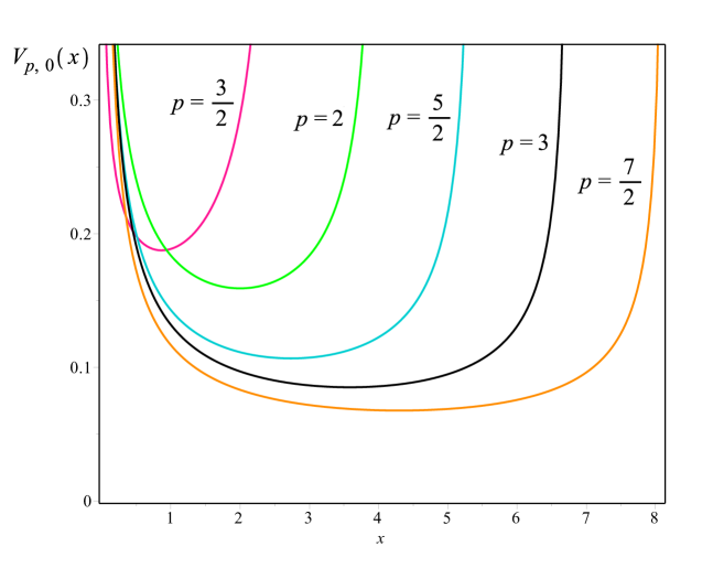
Figure 2. Density functions $V_{p,0}(x)$ for some values of $p$.

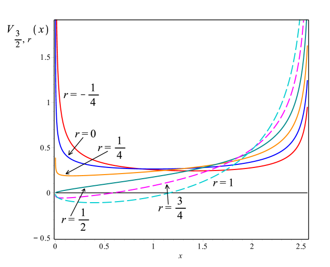
Figure 3. Some examples of $V_{p,r}$ for $p=3/2$. Note that for $r=3/4$ and $1$ the function $V_{3/2,r}(x)$ has also negative values.

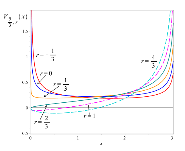
Figure 4. Some examples of $V_{p,r}(x)$ for $p=5/3$.

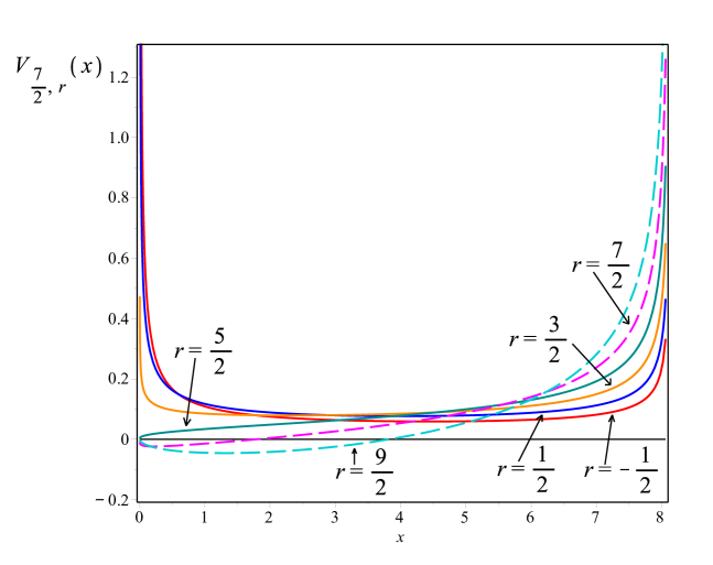
Figure 5. Some examples of $V_{p,r}(x)$ for $p=7/2$.

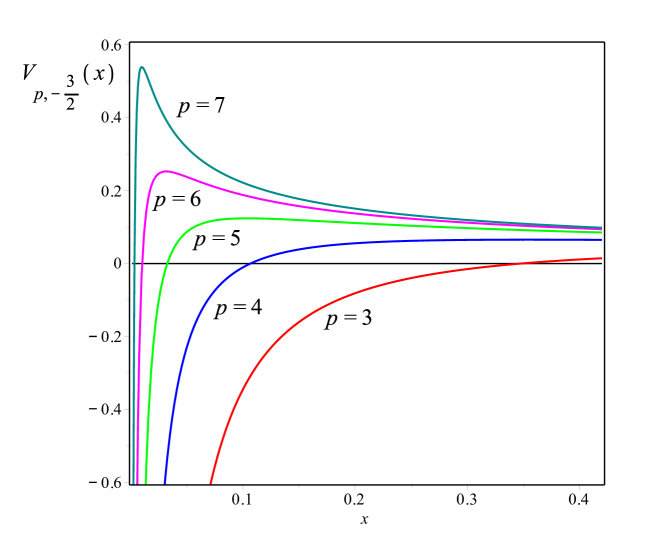
Figure 6. Some examples of $V_{p,r}(x)$ for $r=-3/2$.

8. Graphical illustrations of selected cases

The formulas (48) and (52) alow us to study the graphical representation of the function $V_{p,r}(x)$ for given $p=k/l>1$ and $r\in\mathbb{R}$. Figure 2 shows $V_{p,0}(x)$ for $p=i/2$, $i=3,4,\ldots,7$. Figures 3–5 illustrate $V_{3/2,r}$, $V_{5/3,r}$ and $V_{7/2,r}$ for various choice of $r$, including $r>p-1$ when $V_{p,r}(x)$ is negative for some $x$. Those $V_{p},_{r}$’s which have negative parts are plotted with dashed lines. Finally, in Figure 6, we show graphs of $V_{p,-3/2}(x)$ for some values of $p$. Each of these functions is negative for some values of $x$.

References

- [1] G. E. Andrews, R. Askey, R. Roy, Special Functions, Cambridge University Press, Cambridge 1999.
- [2] N. Balakrishnan, V. B. Nevzorow, A primer on statistical distributions, Wiley-Interscience, Hoboken, New Jersey 2003.
- [3] R. L. Graham, D. E. Knuth, O. Patashnik, Concrete Mathematics. A Foundation for Computer Science, Addison-Wesley, New York 1994.
- [4] O. I. Marichev, Handbook of Integral Transforms of Higher Transcendental Functions-Theory and Algorithmic Tables, Ellis Horwood Ltd, Chichester, 1983.
- [5] W. Młotkowski, Fuss-Catalan numbers in noncommutative probability, Documenta Math. 15 (2010) 939–955.
- [6] W. Młotkowski, K. A. Penson, K. Życzkowski, Densities of the Raney distributions, arXiv:1211.7259.
- [7] N. Muraki, Monotonic independence, monotonic central limit theorem and monotonic law of small numbers, Inf. Dim. Anal. Quantum Probab. Rel. Topics 4 (2001) 39–58.
- [8] A. Nica, R. Speicher, Lectures on the Combinatorics of Free Probability, Cambridge University Press, 2006.
- [9] F. W. J. Olver, D. W. Lozier, R. F. Boisvert, C. W. Clark, NIST Handbook of Mathematical Functions, Cambridge University Press, Cambridge 2010.
- [10] K. A. Penson, K. Życzkowski, Product of Ginibre matrices: Fuss-Catalan and Raney distributions Phys. Rev. E 83 (2011) 061118, 9 pp.
- [11] A. D. Polyanin, A. V. Manzhirov, Handbook of Integral Equations, CRC Press, Boca Raton, 1998.
- [12] A. P. Prudnikov, Yu. A. Brychkov, O. I. Marichev, Integrals and Series, Gordon and Breach, Amsterdam (1998) Vol. 3: More special functions.
- [13] N. J. A. Sloane, The On-line Encyclopedia of Integer Sequences, (2013), published electronically at: http://oeis.org/.
- [14] I. N. Sneddon, The use of integral transforms, Tata Mac Graw-Hill Publishing Company, 1974.
- [15] D. V. Voiculescu, K. J. Dykema, A. Nica, Free random variables, CRM, Montréal, 1992.
- [16] K. Życzkowski, K. A. Penson, I. Nechita, B. Collins, Generating random density matrices, J. Math. Phys. 52 (2011) 062201, 20 pp.