Coherent-Classical Estimation for Quantum Linear Systems

Abstract

This paper introduces a problem of coherent-classical estimation for a class of linear quantum systems. In this problem, the estimator is a mixed quantum-classical system which produces a classical estimate of a system variable. The coherent-classical estimator may also involve coherent feedback. An example involving optical squeezers is given to illustrate the efficacy of this idea.

I Introduction

In recent years, a number of papers have considered the feedback control of systems whose dynamics are governed by the laws of quantum mechanics instead of classical mechanics; see e.g., [1, 2, 3, 4, 5, 6, 7, 8, 9, 10, 11, 12, 13]. Quantum linear systems are an important class of quantum systems; e.g., see [15], [12], [16], [17], [18], [19, 4, 5, 20, 3, 21, 9, 6, 22, 11]). These linear stochastic models describe quantum optical devices such as optical cavities [23], [15], linear quantum amplifiers [16], and finite bandwidth squeezers [16].

Some recent papers on the feedback control of linear quantum systems have considered the case in which the feedback controller itself is also a quantum system. Such feedback control is often referred to as coherent quantum control; e.g., see [24, 25, 4, 5, 26, 7, 8, 21, 27]. In this paper, we consider a related coherent-classical estimation problem in which the estimator consists of a classical part, which produces the final required estimate and a quantum part, which may also involve coherent feedback. A related but different problem is the problem of constructing a quantum observer; see, [28]. A quantum observer is a purely quantum system which aims to produce a quantum estimate of a variable for a given quantum plant. In contrast, we consider a coherent-classical estimator which is a mixed quantum classical system, which produces a classical estimate of a variable for a given quantum plant. We formulate the problem of optimal coherent-classical estimation and then present an example involving optical cavities and dynamic squeezers to show that a coherent-classical estimator may yield improved performance which compared with a classical-only estimator.

II Linear Quantum Systems and Physical Realizability

We consider a class of linear quantum systems described by the quantum stochastic differential equations (QSDEs), (e.g., see [11, 13, 29]):

$$\left[\begin{array}[]{l}da(t)\\ da(t)^{\#}\end{array}\right] = F\left[\begin{array}[]{l}a(t)\\ a(t)^{\#}\end{array}\right]dt+G\left[\begin{array}[]{l}d\mathcal{A}(t)\\ d\mathcal{A}(t)^{\#}\end{array}\right];$$ (7)

$$\left[\begin{array}[]{l}d\mathcal{A}^{out}(t)\\ d\mathcal{A}^{out}(t)^{\#}\end{array}\right] = H\left[\begin{array}[]{l}a(t)\\ a(t)^{\#}\end{array}\right]dt+K\left[\begin{array}[]{l}d\mathcal{A}(t)\\ d\mathcal{A}(t)^{\#}\end{array}\right],$$ (14)

where

$$F=\Delta(F_{1},F_{2}), G=\Delta(G_{1},G_{2}),$$

$$H=\Delta(H_{1},H_{2}), K=\Delta(K_{1},K_{2}).$$ (16)

Here, $a(t)=\left[{a_{1}(t)\cdots a_{n}(t)}\right]^{T}$ is a vector of annihilation operators. The adjoint of the operator $a_{i}$ is denoted by $a_{i}^{*}$ and is referred to as a creation operator. Also, the notation $\Delta(F_{1},F_{2})$ denotes the matrix $\left[\begin{array}[]{cc}F_{1}&F_{2}\\ F_{2}^{\#}&F_{1}^{\#}\end{array}\right]$. Furthermore, ^† denotes the adjoint transpose of a vector of operators or the complex conjugate transpose of a complex matrix. In addition, ^# denotes the adjoint of a vector of operators or the complex conjugate of a complex matrix. Moreover, $F_{1}\in\mathbb{C}^{n\times n}$, $F_{2}\in\mathbb{C}^{n\times n}$, $G_{1}\in\mathbb{C}^{n\times m}$, $G_{2}\in\mathbb{C}^{n\times m}$, $H_{1}\in\mathbb{C}^{m\times n}$, $H_{2}\in\mathbb{C}^{m\times n}$, $K_{1}\in\mathbb{C}^{m\times m}$ and $K_{2}\in\mathbb{C}^{m\times m}$.

The vector $\mathcal{A}=\left[\begin{array}[]{cccc}\mathcal{A}_{1}&\mathcal{A}_{2}&\ldots&\mathcal{A}_{m}\end{array}\right]^{T}$ represents a collection of external independent quantum fields modelled by bosonic annihilation field operators $\mathcal{A}_{1},\mathcal{A}_{2},\ldots,\mathcal{A}_{m}$. Also, the vector $\mathcal{A}^{out}$ represents the corresponding vector of output field operators. For each annihilation field operator $\mathcal{A}_{k}$, there is a corresponding creation field operator $\mathcal{A}_{k}^{*}$, which is the operator adjoint of $\mathcal{A}_{k}$ (see [30], [31] and [32]). More details concerning this class of quantum systems can be found in the references [4, 11, 13, 29].

In the coherent classical filtering problem to be considered in this paper, we require part of the estimator to be a quantum system. In order to achieve this, we will restrict attention to quantum systems described by QSDEs of the form (7), (II) which are physically realizable according to the following definition.

Definition 1

(See [4, 29, 13].) A complex linear quantum system of the form (7), (II) is said to be physically realizable if there exists a complex commutation matrix $\Theta=\Theta^{\dagger}$, a complex Hamiltonian matrix $M=M^{\dagger}$, and a coupling matrix $N$ such that

$$\Theta=TJT^{\dagger}$$ (17)

where $T=\Delta(T_{1},T_{2})$ is non-singular, $M$ and $N$ are of the form

$$M=\Delta(M_{1},M_{2}),N=\Delta(N_{1},N_{2})$$ (18)

and

$$F = -\imath\Theta M-\frac{1}{2}\Theta N^{\dagger}JN;$$

$$G = -\Theta N^{\dagger}J;$$

$$H = N;$$

$$K = I.$$ (19)

In this definition, if the system (7) is physically realizable, then the matrices $M$ and $N$ define a complex open harmonic oscillator with coupling operator

$$L=\left[\begin{array}[]{cc}\tilde{N}_{1}&\tilde{N}_{2}\end{array}\right]\left[\begin{array}[]{c}a\\ a^{\#}\end{array}\right]$$

and a Hamiltonian operator

$$H=\frac{1}{2}\left[\begin{array}[]{cc}a^{\dagger}&a^{T}\end{array}\right]M\left[\begin{array}[]{c}a\\ a^{\#}\end{array}\right];$$

e.g., see [16], [31], [30], [4] and [17]. State space and frequency domain conditions for physical realizability can be found in [4, 29].

III Coherent-Classical Estimation

In this section, we introduce a problem of coherent-classical estimation. In this problem, we begin with a quantum “plant” which is a quantum system of the form (7), (II) defined as follows:

$$\left[\begin{array}[]{l}da(t)\\ da(t)^{\#}\end{array}\right] = F\left[\begin{array}[]{l}a(t)\\ a(t)^{\#}\end{array}\right]dt+G_{1}\left[\begin{array}[]{l}d\mathcal{A}(t)\\ d\mathcal{A}(t)^{\#}\end{array}\right]$$ (29)

$$+G_{2}\left[\begin{array}[]{l}d\mathcal{U}(t)\\ d\mathcal{U}(t)^{\#}\end{array}\right];$$

$$\left[\begin{array}[]{l}d\mathcal{Y}(t)\\ d\mathcal{Y}(t)^{\#}\end{array}\right] = H\left[\begin{array}[]{l}a(t)\\ a(t)^{\#}\end{array}\right]dt+K\left[\begin{array}[]{l}d\mathcal{A}(t)\\ d\mathcal{A}(t)^{\#}\end{array}\right];$$ (36)

$$z = C\left[\begin{array}[]{l}a(t)\\ a(t)^{\#}\end{array}\right].$$ (39)

Here, $z$ denotes a scalar operator on the underlying Hilbert space which represents the quantity to be estimated. Also, $\mathcal{Y}(t)$ represents the vector of output fields of the plant which will be used by the estimator to obtain an estimate of $z$ and $\mathcal{U}(t)$ represents the control input to the plant. As above, $\mathcal{A}(t)$ represents a vector of quantum noises acting on the plant. In the case of a purely classical estimator, the control input is also taken as a vector of quantum noises acting on the plant. Also, in the case of a purely classical estimator, a quadrature of each component of the vector $\mathcal{Y}(t)$ is measured using homodyne detection to produce a corresponding classical signal $y_{i}$; e.g., see [23]. This is represented by the following equations:

$$dy_{1} = \cos(\theta_{1})d\mathcal{Y}_{1}+\sin(\theta_{1})\mathcal{Y}_{1}^{*};$$

$$\vdots$$

$$dy_{m} = \cos(\theta_{m})d\mathcal{Y}_{m}+\sin(\theta_{m})\mathcal{Y}_{m}^{*}.$$ (40)

Here, the angles $\theta_{1},\ldots,\theta_{m}$, determine the quadrature measured by each homodyne detector. The vector of classical signals $y=\left[\begin{array}[]{cccc}y_{1}&y_{2}&\ldots&y_{m}\end{array}\right]^{T}$ is then used as the input to a classical estimator defined as follows:

$$dx_{e} = F_{e}x_{e}dt+G_{e}dy;$$

$$\hat{z} = H_{e}x_{e}.$$ (41)

Here $\hat{z}$ is a scalar classical estimate of the quantity $z$. Corresponding to this estimate is the estimation error

$$e=z-\hat{z}.$$ (42)

Here, $e$ is an operator on the underlying Hilbert space and the second term in the expression for $e$ in (42) is interpreted as the complex number $\hat{z}$ multiplied by the identity operator on the underlying Hilbert space. Then, the optimal classical estimator is defined as the system (III) which minimizes the quantity

$$J=\lim_{t\rightarrow\infty}<e^{*}(t)e(t)>$$ (43)

where $<\cdot>$ denotes the quantum expectation over the joint classical quantum system defined by (29), (III), (III). This problem is illustrated in Figure 1. It is straightforward to verify using a similar approach to that given in [33, 5] that the optimal classical estimator is given by the standard (complex) Kalman filter defined for the system (29), (III).

\psfrag{MA}{$\mathcal{A}$}\psfrag{MU}{$\mathcal{U}$}\psfrag{z0}{$z$}\psfrag{MY}{$\mathcal{Y}$}\psfrag{y0}{$y$}\psfrag{zh}{$\hat{z}$}\includegraphics[width=241.84842pt]{FA.eps}

Figure 1: Quantum estimation using a purely classical estimator.

We now extend this problem to case of a coherent-classical estimator. In the case of coherent-classical estimation, we do not feed the plant output $\mathcal{Y}(t)$ directly into a bank of homodyne detectors as in (III) but rather, we feed this output into another quantum system referred to as a coherent controller, which also provides coherent feedback control to the quantum plant. This coherent controller is defined as follows:

$$\left[\begin{array}[]{l}da_{c}(t)\\ da_{c}(t)^{\#}\end{array}\right] = F_{c}\left[\begin{array}[]{l}a_{c}(t)\\ a_{c}(t)^{\#}\end{array}\right]dt+G_{c1}\left[\begin{array}[]{l}d\mathcal{\tilde{A}}(t)\\ d\mathcal{\tilde{A}}(t)^{\#}\end{array}\right];$$ (53)

$$+G_{c2}\left[\begin{array}[]{l}d\mathcal{Y}(t)\\ d\mathcal{Y}(t)^{\#}\end{array}\right];$$

$$\left[\begin{array}[]{l}d\mathcal{\tilde{Y}}(t)\\ d\mathcal{\tilde{Y}}(t)^{\#}\end{array}\right] = \tilde{H}_{c}\left[\begin{array}[]{l}a_{c}(t)\\ a_{c}(t)^{\#}\end{array}\right]dt+\tilde{K}_{c1}\left[\begin{array}[]{l}d\mathcal{\tilde{A}}(t)\\ d\mathcal{\tilde{A}}(t)^{\#}\end{array}\right]$$ (63)

$$+\tilde{K}_{c2}\left[\begin{array}[]{l}d\mathcal{Y}(t)\\ d\mathcal{Y}(t)^{\#}\end{array}\right];$$

$$\left[\begin{array}[]{l}d\mathcal{U}(t)\\ d\mathcal{U}(t)^{\#}\end{array}\right] = H_{c}\left[\begin{array}[]{l}a_{c}(t)\\ a_{c}(t)^{\#}\end{array}\right]dt+K_{c1}\left[\begin{array}[]{l}d\mathcal{\tilde{A}}(t)\\ d\mathcal{\tilde{A}}(t)^{\#}\end{array}\right]$$ (73)

$$+K_{c2}\left[\begin{array}[]{l}d\mathcal{Y}(t)\\ d\mathcal{Y}(t)^{\#}\end{array}\right].$$

Here, $\mathcal{\tilde{A}}$ represents an additional quantum noise acting on the quantum part of the coherent-classical estimator and $\mathcal{\tilde{Y}}$ represents its estimation output field. Note that the dimension of the estimation output field vector $\mathcal{\tilde{Y}}$ may be different from the dimension of the field vector $\mathcal{Y}$. The quantum system (53) is required to be physically realizable. Note, that in order to meet the definition of physical realizability in Definition 1, it may be necessary to augment this system with some additional unused output fields; see also [8, 34].

A quadrature of each component of the vector $\mathcal{\tilde{Y}}(t)$ is measured using homodyne detection to produce a corresponding classical signal $\tilde{y}_{i}$; e.g., see [23]. This is represented by the following equations:

$$d\tilde{y}_{1} = \cos(\tilde{\theta}_{1})d\mathcal{\tilde{Y}}_{1}+\sin(\tilde{\theta}_{1})\mathcal{\tilde{Y}}_{1}^{*};$$

$$\vdots$$

$$d\tilde{y}_{\tilde{m}} = \cos(\tilde{\theta}_{\tilde{m}})d\mathcal{\tilde{Y}}_{\tilde{m}}+\sin(\tilde{\theta}_{\tilde{m}})\mathcal{\tilde{Y}}_{\tilde{m}}^{*}.$$ (75)

Here, the angles $\tilde{\theta}_{1},\ldots,\tilde{\theta}_{\tilde{m}}$, determine the quadrature measured by each homodyne detector. The vector of classical signals $\tilde{y}=\left[\begin{array}[]{cccc}\tilde{y}_{1}&\tilde{y}_{2}&\ldots&\tilde{y}_{\tilde{m}}\end{array}\right]^{T}$ is then used as the input to a classical estimator defined as follows:

$$d\tilde{x}_{e} = \tilde{F}_{e}\tilde{x}_{e}dt+\tilde{G}_{e}d\tilde{y};$$

$$\hat{z} = \tilde{H}_{e}\tilde{x}_{e}.$$ (76)

Here $\hat{z}$ is a scalar classical estimate of the quantity $z$. Corresponding to this estimate is the estimation error (42). Then, the optimal coherent-classical estimator is defined as the systems (53), (III) which together minimize the quantity (43). This problem is illustrated in Figure 2. Note that the coherent controller is not required to directly produce an estimate of the variables of the quantum plant as in the quantum observer considered in [28]. Rather, the coherent controller works only in combination with the classical estimator to produce a classical estimate of the quantity $z$.

\psfrag{MA0}{$\mathcal{A}$}\psfrag{MU0}{$\mathcal{U}$}\psfrag{MAT}{$\mathcal{\tilde{A}}$}\psfrag{z0}{$z$}\psfrag{MY0}{$\mathcal{Y}$}\psfrag{MYT}{$\mathcal{\tilde{Y}}$}\psfrag{y0}{$\tilde{y}$}\psfrag{zh}{$\hat{z}$}\includegraphics[width=241.84842pt]{FB.eps}

Figure 2: Quantum estimation using a coherent-classical estimator.

We can now combine the quantum plant (29) and the coherent controller (53) to yield a closed loop quantum linear system defined by the following QSDEs:

$$\left[\begin{array}[]{l}da\\ da^{\#}\\ da_{c}\\ da_{c}^{\#}\end{array}\right] = \left[\begin{array}[]{cc}F+G_{2}K_{c2}H&G_{2}H_{c}\\ G_{c2}H&F_{c}\end{array}\right]\left[\begin{array}[]{l}a\\ a^{\#}\\ a_{c}\\ a_{c}^{\#}\end{array}\right]dt$$

$$+\left[\begin{array}[]{cc}G_{1}+G_{2}K_{c2}K&G_{2}K_{c1}\\ G_{c2}K&G_{c1}\end{array}\right]\left[\begin{array}[]{l}d\mathcal{A}\\ d\mathcal{A}^{\#}\\ d\mathcal{\tilde{A}}\\ d\mathcal{\tilde{A}}^{\#}\end{array}\right];$$

$$\left[\begin{array}[]{l}d\mathcal{\tilde{Y}}\\ d\mathcal{\tilde{Y}}^{\#}\end{array}\right] = \left[\begin{array}[]{cc}\tilde{K}_{c2}H&\tilde{H}_{c}\end{array}\right]\left[\begin{array}[]{l}a\\ a^{\#}\\ a_{c}\\ a_{c}^{\#}\end{array}\right]dt$$ (92)

$$+\left[\begin{array}[]{cc}\tilde{K}_{c2}K&\tilde{K}_{c1}\end{array}\right]\left[\begin{array}[]{l}d\mathcal{A}\\ d\mathcal{A}^{\#}\\ d\mathcal{\tilde{A}}\\ d\mathcal{\tilde{A}}^{\#}\end{array}\right].$$

Once the coherent controller (53) has been determined, it is straightforward to verify using a similar approach to that given in [33, 5] that the optimal classical estimator (III) is given by the standard (complex) Kalman filter defined for the system (92), (III). Indeed, this optimal classical estimator is obtained from the stabilizing solution to the algebraic Riccati equation

$$F_{a}P+PF_{a}^{\dagger}+G_{a}G_{a}^{\dagger}$$ (94)

$$-(G_{a}K_{a}^{\dagger}+PH_{a}^{\dagger})L^{\dagger}(LK_{a}K_{a}^{\dagger}L^{\dagger})^{-1}(G_{a}K_{a}^{\dagger}+PH_{a}^{\dagger})^{\dagger}$$

$$= 0$$

where

$$F_{a} = \left[\begin{array}[]{cc}F+G_{2}K_{c2}H&G_{2}H_{c}\\ G_{c2}H&F_{c}\end{array}\right];$$ (97)

$$G_{a} = \left[\begin{array}[]{cc}G_{1}+G_{2}K_{c2}K&G_{2}K_{c1}\\ G_{c2}K&G_{c1}\end{array}\right];$$ (100)

$$H_{a} = \left[\begin{array}[]{cc}\tilde{K}_{c2}H&\tilde{H}_{c}\end{array}\right];~{}~{}K_{a}=\left[\begin{array}[]{cc}\tilde{K}_{c2}K&\tilde{K}_{c1}\end{array}\right];$$ (103)

$$L = \left[\begin{array}[]{cc}L_{1}&L_{2}\end{array}\right];$$ (105)

$$L_{1} = \left[\begin{array}[]{cccc}\cos(\tilde{\theta}_{1})&0&\ldots&0\\ 0&\cos(\tilde{\theta}_{2})&\ldots&0\\ &&\ddots&\\ &&&\cos(\tilde{\theta}_{\tilde{m}})\end{array}\right];$$ (110)

$$L_{2} = \left[\begin{array}[]{cccc}\sin(\tilde{\theta}_{1})&0&\ldots&0\\ 0&\sin(\tilde{\theta}_{2})&\ldots&0\\ &&\ddots&\\ &&&\sin(\tilde{\theta}_{\tilde{m}})\end{array}\right];$$ (115)

e.g., see [35]. Here we assume that the quantum noises $\mathcal{A}$ and $\mathcal{\tilde{A}}$ are independent and purely canonical; i.e., $d\mathcal{A}d\mathcal{A}^{\dagger}=Idt$ and $d\mathcal{\tilde{A}}d\mathcal{\tilde{A}}^{\dagger}=Idt$ (e.g., see [8]). Then, the corresponding optimal classical estimator (III) is defined by the equations:

$$\tilde{F}_{e} = F_{a}-G_{e}LH_{a};$$

$$\tilde{G}_{e} = (G_{a}K_{a}^{\dagger}+PH_{a}^{\dagger})L^{\dagger}(LK_{a}K_{a}^{\dagger}L^{\dagger})^{-1};$$

$$\tilde{H}_{e} = \left[\begin{array}[]{cc}C&0\end{array}\right];$$ (117)

e.g., see [35]. The corresponding value of the cost (43) is given by

$$J=\left[\begin{array}[]{cc}C&0\end{array}\right]P\left[\begin{array}[]{c}C^{\dagger}\\ 0\end{array}\right]$$ (118)

where $P$ is the stabilizing solution to the algebraic Riccati equation (94). Thus, the optimal coherent-classical estimation problem can be solved by first choosing the coherent controller (53) to minimize the cost (118). Then, the classical estimator (III) is constructed according to the equations (III).

A simple example of a coherent-classical estimator arises in the case in which the plant output $\mathcal{Y}$ is a scalar operator and the coherent controller is simply a beam splitter and no feedback is used as shown in Figure 3.

\psfrag{MA0}{$\mathcal{A}$}\psfrag{MU0}{$\mathcal{U}$}\psfrag{MAT}{$\mathcal{\tilde{A}}$}\psfrag{z0}{$z$}\psfrag{MY0}{$\mathcal{Y}$}\psfrag{MYT1}{$\mathcal{\tilde{Y}}_{1}$}\psfrag{MYT2}{$\mathcal{\tilde{Y}}_{2}$}\psfrag{y0}{$\tilde{y}$}\psfrag{zh}{$\hat{z}$}\includegraphics[width=241.84842pt]{FC.eps}

Figure 3: Coherent-classical estimation using a beam splitter.

This approach is commonly referred to as dual homodyne measurement. Furthermore, it is related to an equivalent method referred to as heterodyne measurement; e.g., see [23]. Hence, this approach is also referred to as heterodyne measurement. However, it is well known that this approach does not lead to any advantages over the purely classical estimation approach described above. In the next section, we consider the case in which the coherent controller is a dynamic squeezer and feedback is used. We show that this does lead to advantages over the purely classical estimation approach.

IV Dynamic Squeezer Systems

In this section, we illustrate the notion of coherent-classical estimation by a simple example involving the use of a dynamic quantum squeezer as a coherent controller; e.g., see [36]. This example shows that the process of coherent-classical estimation has the potential to yield improved performance compared with purely classical estimation.

An optical cavity consists of partially reflecting mirrors arranged to produce a cavity mode when coupled to a coherent light source; e.g., see [23, 16]. By including a nonlinear optical element inside such a cavity, an optical squeezer can be obtained. By using suitable linearizations and approximations, such an optical squeezer can be described by the following quantum stochastic differential equations:

$$da = -\frac{\gamma}{2}adt-\chi a^{*}dt-\sqrt{\kappa_{1}}d\mathcal{A}_{1}-\sqrt{\kappa_{2}}d\mathcal{A}_{3};$$

$$d\mathcal{A}_{1}^{out} = \sqrt{\kappa_{1}}adt+d\mathcal{A}_{1};$$

$$d\mathcal{A}_{2}^{out} = \sqrt{\kappa_{2}}adt+d\mathcal{A}_{2};$$ (119)

where $\kappa_{1}>0$, $\kappa_{2}>0$, $\gamma=\kappa_{1}+\kappa_{2}$, $\chi\in\mathbb{C}$, and $a$ is a single annihilation operator associated with the cavity mode; e.g., see [23, 16]. This leads to a linear quantum system of the form (7) as follows:

$$\left[\begin{array}[]{l}da(t)\\ da(t)^{*}\end{array}\right] = \left[\begin{array}[]{ll}-\frac{\gamma}{2}&-\chi\\ -\chi^{*}&-\frac{\gamma}{2}\end{array}\right]\left[\begin{array}[]{l}a(t)\\ a(t)^{*}\end{array}\right]dt$$ (132)

$$-\sqrt{\kappa_{1}}\left[\begin{array}[]{l}d\mathcal{A}_{1}(t)\\ d\mathcal{A}_{2}(t)^{\#}\end{array}\right];$$

$$-\sqrt{\kappa_{2}}\left[\begin{array}[]{l}d\mathcal{A}_{2}(t)\\ d\mathcal{A}_{2}(t)^{\#}\end{array}\right];$$

$$\left[\begin{array}[]{l}d\mathcal{A}_{1}^{out}(t)\\ d\mathcal{A}_{1}^{out}(t)^{\#}\end{array}\right] = \sqrt{\kappa_{1}}\left[\begin{array}[]{l}a(t)\\ a(t)^{*}\end{array}\right]dt+\left[\begin{array}[]{l}d\mathcal{A}_{1}(t)\\ d\mathcal{A}_{1}(t)^{\#}\end{array}\right];$$ (139)

$$\left[\begin{array}[]{l}d\mathcal{A}_{2}^{out}(t)\\ d\mathcal{A}_{2}^{out}(t)^{\#}\end{array}\right] = \sqrt{\kappa_{2}}\left[\begin{array}[]{l}a(t)\\ a(t)^{*}\end{array}\right]dt+\left[\begin{array}[]{l}d\mathcal{A}_{2}(t)\\ d\mathcal{A}_{2}(t)^{\#}\end{array}\right].$$ (146)

Also associated with the squeezer system is the position operator $q=a+a^{*}$ and the momentum operator $p=\frac{a-a^{*}}{\imath}$.

The construction of an optical squeezer is illustrated in Figure 4.

Figure 4: An optical squeezer system.

Such an optical squeezer is often represented as shown in the diagram in Figure 5.

\psfrag{a}{$a$}\psfrag{A1}{$\mathcal{A}_{1}$}\psfrag{Ao1}{$\mathcal{A}_{1}^{out}$}\psfrag{A2}{$\mathcal{A}_{2}$}\psfrag{Ao2}{$\mathcal{A}_{2}^{out}$}\includegraphics[width=170.71652pt]{F2.eps}

Figure 5: Squeezer schematic diagram.

We now consider a quantum plant of the form (29) corresponding to a dynamic quantum squeezer. This system is described by the QSDEs

$$\left[\begin{array}[]{l}da(t)\\ da(t)^{*}\end{array}\right] = \left[\begin{array}[]{ll}-\frac{\gamma}{2}&-\chi\\ -\chi^{*}&-\frac{\gamma}{2}\end{array}\right]\left[\begin{array}[]{l}a(t)\\ a(t)^{*}\end{array}\right]dt$$ (160)

$$-\sqrt{\kappa_{1}}\left[\begin{array}[]{l}d\mathcal{A}(t)\\ d\mathcal{A}(t)^{\#}\end{array}\right];$$

$$-\sqrt{\kappa_{2}}\left[\begin{array}[]{l}d\mathcal{U}(t)\\ d\mathcal{U}(t)^{\#}\end{array}\right];$$

$$\left[\begin{array}[]{l}d\mathcal{Y}(t)\\ d\mathcal{Y}(t)^{\#}\end{array}\right] = \sqrt{\kappa_{1}}\left[\begin{array}[]{l}a(t)\\ a(t)^{*}\end{array}\right]dt+\left[\begin{array}[]{l}d\mathcal{A}(t)\\ d\mathcal{A}(t)^{\#}\end{array}\right];$$ (167)

$$z = \left[\begin{array}[]{ll}\frac{1}{\sqrt{2}}&-\frac{1}{\sqrt{2}}\end{array}\right].$$ (169)

This choice of $z$ corresponds to a scaled version of the momentum operator. We consider the case of $\chi=0$ and $\kappa_{1}=0.5$, $\kappa_{2}=0.5$, $\gamma=1$. This case corresponds to a standard optical cavity without any squeezing. The matrices corresponding to the system (29) are

$$F = \left[\begin{array}[]{ll}-0.5&0\\ 0&-0.5\end{array}\right];$$

$$G_{1} = \left[\begin{array}[]{ll}-0.7071&0\\ 0&-0.7071\end{array}\right];$$

$$G_{2} = \left[\begin{array}[]{ll}-0.7071&0\\ 0&-0.7071\end{array}\right];$$

$$H = \left[\begin{array}[]{ll}0.7071&0\\ 0&0.7071\end{array}\right];$$

$$K = \left[\begin{array}[]{ll}1&0\\ 0&1\end{array}\right];~{}C=\left[\begin{array}[]{ll}0.7071&-0.7071\end{array}\right].$$

We then calculate the optimal classical only state estimator for this system using the standard Kalman filter equations (e.g., see [35]) corresponding to a homodyne detector angle of $\theta=135^{\circ}$; i.e., measuring the momentum quadrature of $\mathcal{\tilde{Y}}$. This case is illustrated in Figure 6.

\psfrag{a}{$a$}\psfrag{MA0}{$\mathcal{A}$}\psfrag{MU}{$\mathcal{U}$}\psfrag{MAT}{$\mathcal{\tilde{A}}$}\psfrag{MY}{$\mathcal{Y}$}\psfrag{yt}{$\tilde{y}$}\psfrag{zh}{$\hat{z}$}\includegraphics[width=241.84842pt]{F2a.eps}

Figure 6: Classical only estimation for an optical cavity plant.

The optimal classical only state estimator for this system leads to an error (43) of $J=1$. This is the same as the covariance of the variable $z$ without measurement. Also, the Kalman gain $G_{e}$ is found to be zero. That is, the measurement contains no information about the quantity $z$ to be estimated. This is consistent with Corollary 1 of [34] which notes that for a physically realizable annihilation operator system with only quantum noise inputs, any output field contains no information about the internal variables of the system. A similar result is found with any other homodyne detector angle $\theta$ as shown in Figure 7.

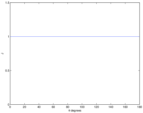
Figure 7: Estimation error covariance versus homodyne detection angle $\theta$ for the case of classical only estimation.

We now consider the case in which a dynamic squeezer is used as the coherent controller in a coherent-classical estimation scheme. In this case, the coherent controller (53) is described by the equations

$$\left[\begin{array}[]{l}da(t)\\ da(t)^{*}\end{array}\right] = \left[\begin{array}[]{ll}-\frac{\gamma}{2}&-\chi\\ -\chi^{*}&-\frac{\gamma}{2}\end{array}\right]\left[\begin{array}[]{l}a(t)\\ a(t)^{*}\end{array}\right]dt$$ (187)

$$-\sqrt{\kappa_{1}}\left[\begin{array}[]{l}d\mathcal{\tilde{A}}(t)\\ d\mathcal{\tilde{A}}(t)^{\#}\end{array}\right];$$

$$-\sqrt{\kappa_{2}}\left[\begin{array}[]{l}d\mathcal{Y}(t)\\ d\mathcal{Y}(t)^{\#}\end{array}\right];$$

$$\left[\begin{array}[]{l}d\mathcal{\tilde{Y}}(t)\\ d\mathcal{\tilde{Y}}(t)^{\#}\end{array}\right] = \sqrt{\kappa_{1}}\left[\begin{array}[]{l}a(t)\\ a(t)^{*}\end{array}\right]dt+\left[\begin{array}[]{l}d\mathcal{\tilde{A}}(t)\\ d\mathcal{\tilde{A}}(t)^{\#}\end{array}\right];$$ (194)

$$\left[\begin{array}[]{l}d\mathcal{U}(t)\\ d\mathcal{U}(t)^{\#}\end{array}\right] = \sqrt{\kappa_{2}}\left[\begin{array}[]{l}a(t)\\ a(t)^{*}\end{array}\right]dt+\left[\begin{array}[]{l}d\mathcal{Y}(t)\\ d\mathcal{Y}(t)^{\#}\end{array}\right].$$ (201)

Here, we choose $\chi=-0.5$ and $\kappa_{1}=5$, $\kappa_{2}=5$, $\gamma=10$. The matrices corresponding to the system (53) are

$$F_{c} = \left[\begin{array}[]{ll}-5&-0.5\\ -0.5&-5\end{array}\right];$$

$$G_{c1} = \left[\begin{array}[]{ll}-2.2361&0\\ 0&-2.2361\end{array}\right];$$

$$G_{c2} = \left[\begin{array}[]{ll}-2.2361&0\\ 0&-2.2361\end{array}\right];$$

$$\tilde{H}_{c} = \left[\begin{array}[]{ll}2.2361&0\\ 0&2.2361\end{array}\right];$$

$$\tilde{K}_{c1} = \left[\begin{array}[]{ll}1&0\\ 0&1\end{array}\right];~{}~{}\tilde{K}_{c2}=0;$$

$$H_{c} = \left[\begin{array}[]{ll}2.2361&0\\ 0&2.2361\end{array}\right];~{}~{}K_{c1}=0;$$

$$K_{c2} = \left[\begin{array}[]{ll}1&0\\ 0&1\end{array}\right].$$

Then, the classical state estimator for this case is calculated according to equations (97), (94), (III) for different values of the homodyne detector angle $\theta$. This case is illustrated in Figure 8. The resulting value of the cost $J$ in (43) along with the cost for the classical only estimator case is shown in Figure 9.

\psfrag{a}{$a$}\psfrag{ac}{$a_{c}$}\psfrag{MA0}{$\mathcal{A}$}\psfrag{MU}{$\mathcal{U}$}\psfrag{MAT}{$\mathcal{\tilde{A}}$}\psfrag{MY}{$\mathcal{Y}$}\psfrag{MYT}{$\mathcal{\tilde{Y}}$}\psfrag{yt}{$\tilde{y}$}\psfrag{zh}{$\hat{z}$}\includegraphics[width=241.84842pt]{F3a.eps}

Figure 8: Coherent-classical estimation for an optical cavity plant.

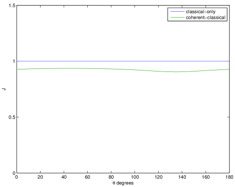
Figure 9: Estimation error covariance versus homodyne detection angle $\theta$ for the case of coherent-classical estimation.

From this figure, we can see that the coherent-classical estimator performs better than the classical only estimator with the best performance being achieved at a homodyne detector angle of $\theta=135^{\circ}$ which corresponds to measuring the momentum quadrature of the field $\mathcal{\tilde{Y}}$. Note that a critical feature of this coherent-classical estimator is the use of coherent feedback. It does not seem possible to obtain improved performance with a coherent-classical estimator without the use of such feedback.

V Conclusions

In this paper, we have introduced the problem of classical-coherent estimation for quantum systems and shown via an example involving dynamic squeezers that the use of classical-coherent estimators can lead to significant improvement over the use of classical only estimators.

References

- [1] M. Yanagisawa and H. Kimura, “Transfer function approach to quantum control-part I: Dynamics of quantum feedback systems,” IEEE Transactions on Automatic Control, vol. 48, no. 12, pp. 2107–2120, 2003.
- [2] ——, “Transfer function approach to quantum control-part II: Control concepts and applications,” IEEE Transactions on Automatic Control, vol. 48, no. 12, pp. 2121–2132, 2003.
- [3] N. Yamamoto, “Robust observer for uncertain linear quantum systems,” Phys. Rev. A, vol. 74, pp. 032 107–1 – 032 107–10, 2006.
- [4] M. R. James, H. I. Nurdin, and I. R. Petersen, “ control of linear quantum stochastic systems,” IEEE Transactions on Automatic Control, vol. 53, no. 8, pp. 1787–1803, 2008.
- [5] H. I. Nurdin, M. R. James, and I. R. Petersen, “Coherent quantum LQG control,” Automatica, vol. 45, no. 8, pp. 1837–1846, 2009.
- [6] J. Gough, R. Gohm, and M. Yanagisawa, “Linear quantum feedback networks,” Physical Review A, vol. 78, p. 062104, 2008.
- [7] A. I. Maalouf and I. R. Petersen, “Bounded real properties for a class of linear complex quantum systems,” IEEE Transactions on Automatic Control, vol. 56, no. 4, pp. 786 – 801, 2011.
- [8] ——, “Coherent control for a class of linear complex quantum systems,” IEEE Transactions on Automatic Control, vol. 56, no. 2, pp. 309–319, 2011.
- [9] N. Yamamoto, H. I. Nurdin, M. R. James, and I. R. Petersen, “Avoiding entanglement sudden-death via feedback control in a quantum network,” Physical Review A, vol. 78, no. 4, p. 042339, 2008.
- [10] J. Gough and M. R. James, “The series product and its application to quantum feedforward and feedback networks,” IEEE Transactions on Automatic Control, vol. 54, no. 11, pp. 2530–2544, 2009.
- [11] J. E. Gough, M. R. James, and H. I. Nurdin, “Squeezing components in linear quantum feedback networks,” Physical Review A, vol. 81, p. 023804, 2010.
- [12] H. M. Wiseman and G. J. Milburn, Quantum Measurement and Control. Cambridge University Press, 2010.
- [13] I. R. Petersen, “Quantum linear systems theory,” in Proceedings of the 19th International Symposium on Mathematical Theory of Networks and Systems, Budapest, Hungary, July 2010.
- [14] M. James and J. Gough, “Quantum dissipative systems and feedback control design by interconnection,” IEEE Transactions on Automatic Control, vol. 55, no. 8, pp. 1806 –1821, August 2010.
- [15] D. F. Walls and G. J. Milburn, Quantum Optics. Berlin; New York: Springer-Verlag, 1994.
- [16] C. Gardiner and P. Zoller, Quantum Noise. Berlin: Springer, 2000.
- [17] S. C. Edwards and V. P. Belavkin, “Optimal quantum feedback control via quantum dynamic programming,” University of Nottingham,” quant-ph/0506018, 2005.
- [18] V. P. Belavkin and S. C. Edwards, “Quantum filtering and optimal control,” in Quantum Stochastics and Information: Statistics, Filtering and Control (University of Nottingham, UK, 15 - 22 July 2006), V. P. Belavkin and M. Guta, Eds. Singapore: World Scientific, 2008.
- [19] H. M. Wiseman and A. C. Doherty, “Optimal unravellings for feedback control in linear quantum systems,” Physics Review Letters, vol. 94, pp. 070 405–1 – 070 405–1, 2005.
- [20] H. I. Nurdin, M. R. James, and A. C. Doherty, “Network synthesis of linear dynamical quantum stochastic systems,” SIAM Journal on Control and Optimization, vol. 48, no. 4, pp. 2686–2718, 2009.
- [21] H. Mabuchi, “Coherent-feedback quantum control with a dynamic compensator,” Physical Review A, vol. 78, p. 032323, 2008.
- [22] G. Sarma, A. Silberfarb, and H. Mabuchi, “Quantum stochastic calculus approach to modeling double-pass atom-field coupling,” Physical Review A, vol. 78, p. 025801, 2008.
- [23] H. Bachor and T. Ralph, A Guide to Experiments in Quantum Optics, 2nd ed. Weinheim, Germany: Wiley-VCH, 2004.
- [24] H. M. Wiseman and G. J. Milburn, “All-optical versus electro-optical quantum-limited feedback,” Physical Review A, vol. 49, no. 5, pp. 4110–4125, 1994.
- [25] S. Lloyd, “Coherent quantum feedback,” Physical Review A, vol. 62, no. 022108, 2000.
- [26] A. I. Maalouf and I. R. Petersen, “Coherent control for a class of linear complex quantum systems.” in 2009 American Control Conference, St Louis, Mo, June 2009.
- [27] J. E. Gough and S. Wildfeuer, “Enhancement of field squeezing using coherent feedback,” Physical Review A, vol. 80, p. 042107, 2009.
- [28] Z. Miao and M. R. James, “Quantum observer for linear quantum stochastic systems,” in Proceedings of the 51st IEEE Conference on Decision and Control, Maui, December 2012.
- [29] A. J. Shaiju and I. R. Petersen, “A frequency domain condition for the physical realizability of linear quantum systems,” IEEE Transactions on Automatic Control, vol. 57, no. 8, pp. 2033 – 2044, 2012.
- [30] L. Bouten, R. van Handel, and M. James, “An introduction to quantum filtering,” SIAM J. Control and Optimization, vol. 46, no. 6, pp. 2199–2241, 2007.
- [31] K. Parthasarathy, An Introduction to Quantum Stochastic Calculus. Berlin: Birkhauser, 1992.
- [32] R. Hudson and K. Parthasarathy, “Quantum Ito’s formula and stochastic evolution,” Communications in Mathematical Physics, vol. 93, pp. 301–323, 1984.
- [33] A. J. Shaiju, I. R. Petersen, and M. R. James, “Guaranteed cost LQG control of uncertain linear stochastic quantum systems,” in Proceedings of the 2007 American Control Conference, New York, July 2007.
- [34] I. R. Petersen, “Notes on coherent feedback control for linear quantum systems,” in Australian Control Conference, Perth, Australia, November 2013, submitted.
- [35] H. Kwakernaak and R. Sivan, Linear Optimal Control Systems. Wiley, 1972.
- [36] I. R. Petersen, “Realization of single mode quantum linear systems using static and dynamic squeezers,” in Proceedings of the 8th Asian Control Conference, Kaohsiung, Taiwan, May 2011.