Non-abelian Weyl Commutation Relations and the Series Product of Quantum Stochastic Evolutions

Abstract

We show that the series product, which serves as an algebraic rule for connecting state-based input/output systems, is intimately related to the Heisenberg group and the canonical commutation relations. The series product for quantum stochastic models then corresponds to a non-abelian generalization of the Weyl commutation relation. We show that the series product gives the general rule for combining the generators of quantum stochastic evolutions using a Lie-Trotter product formula.

1 Introduction

The aim of this paper is to make some striking connections between the rules for combining models in series in control system theory and the Weyl commutation relations. In the process, we develop a more intrinsic view of the unitary adapted processes of Hudson and Parthasarathy [1] as non-abelian versions of the Weyl unitaries - where the non-abelian nature arises from the presence of the initial space. Our starting point is a surprising connection between the theory of classical linear state space models and the canonical commutation relations.

1.1 State-Based Input/Output Systems

Let $\mathcal{X},\mathcal{U}$ and $\mathcal{Y}$ be finite dimensional vector spaces over the reals. A controlled flow on the state space $\mathcal{X}$ is given by the dynamical equations

$$\dot{x}=v\left(x,u\right)$$

where $u$ is a $\mathcal{U}$-valued function of time called the input process. An output process $y$ taking values in $\mathcal{Y}$ is given by some relation of the general form

$$y=h\left(x,u\right).$$

The situation is sketched in figure 1, along with the case where we further decompose the value spaces into subspaces.

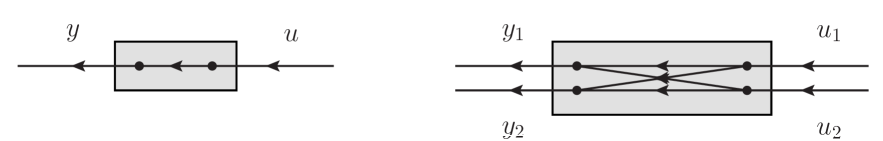
Figure 1: The left-hand picture sketches an input-state-output model $\left(\mathcal{U},\mathcal{X},\mathcal{Y}\right)$ corresponding to the system of equations (1). On the right we consider decompositions of the input and output value spaces, $\mathcal{U}=\mathcal{U}_{1}\oplus\mathcal{U}_{2}$ and $\mathcal{Y}=\mathcal{Y}_{1}\oplus\mathcal{Y}_{2}$ respectively.

1.2 Linear Systems

We consider a vector input $u\left(\cdot\right)$ leading to a vector output $y\left(\cdot\right)$ according to the model

$$\left\{\begin{array}[]{c}\dot{x}=Kx+Lu;\\ y=Mx+Nu;\end{array}\right.$$ (1)

or

$$\left[\begin{array}[]{c}\dot{x}\\ y\end{array}\right]=\mathbf{V}\left[\begin{array}[]{c}x\\ u\end{array}\right]\text{, where }\mathbf{V}=\left[\begin{array}[]{cc}K&M\\ L&N\end{array}\right].$$

Here $x\left(\cdot\right)$ is the state vector state, initialized at some value $x_{0}$, and $\mathbf{V}$ is referred to as the model matrix for the model. For $u\left(\cdot\right)$ integrable, the solution can be written immediately as $y\left(t\right)=Nu\left(t\right)+\int_{0}^{t}Me^{K\left(t-s\right)}Lu(s)ds+Me^{Kt}x_{0}$: we also note that the input-output relation is described by the transfer function $T\left(s\right)=N+M\left(sI-K\right)^{-1}L$ which is determined from the model matrix. The situation is sketched in the top left picture in figure 2.

As the inputs and outputs are vector-valued they may be further decomposed as say $u=\left[\begin{array}[]{c}u_{1}\\ u_{2}\end{array}\right]$ and $y=\left[\begin{array}[]{c}y_{1}\\ y_{2}\end{array}\right]$. This is sketched on the right in figure 2. The model matrix is then

$$\mathbf{V}=\left[\begin{array}[]{cc}K&[M_{1},M_{2}]\\ \left[\begin{array}[]{c}L_{1}\\ L_{2}\end{array}\right]&\left[\begin{array}[]{cc}N_{11}&N_{12}\\ N_{21}&N_{22}\end{array}\right]\end{array}\right].$$ (2)

In each case we have a port for each input/output. The lines external to the block represent an input or output, while the lines internal to the block correspond to a non-zero entry $N_{ij}$ connect input port $j$ to output port $i$. The picture on the bottom of figure 2 sketches the situation where $N_{12}=N_{21}=0$.

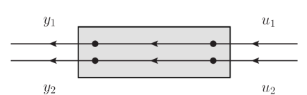
Figure 2: The picture sketches the situation in (2) where $N_{12}=N_{21}=0$.

1.3 Concatenation

Suppose that we have a pair of such models with the same state space (with variable $x$) and model matrices $\mathbf{V}_{i}=\left[\begin{array}[]{cc}K_{i}&M_{i}\\ L_{i}&N_{i}\end{array}\right]$, that is,

$$\left[\begin{array}[]{c}\dot{x}\\ y_{2}\end{array}\right]=\mathbf{V}_{2}\left[\begin{array}[]{c}x\\ u_{2}\end{array}\right],\quad\left[\begin{array}[]{c}\dot{x}\\ y_{1}\end{array}\right]=\mathbf{V}_{1}\left[\begin{array}[]{c}x\\ u_{1}\end{array}\right].$$

We may superimpose the two models to get the concatenated model

$$\left\{\begin{array}[]{l}\dot{x}=\left(K_{1}+K_{2}\right)x+M_{1}u_{1}+M_{2}u_{2},\\ y_{1}=L_{1}x+N_{1}u_{1},\\ y_{2}=L_{2}x+N_{2}u_{2},\end{array}\right.$$

- writing $v_{i}(x)=K_{i}x+M_{i}u_{i}$ for the separate state velocity fields ($i=1,2$), the concatenation rule effectively takes the combined velocity field

$$v(x)=v_{1}(x)+v_{2}(x).$$ (3)

At the level of model matrices, this corresponds to the rule (see figure 3)

$$\mathbf{V}_{1}\boxplus\mathbf{V}_{2}\triangleq\left[\begin{array}[]{ccc}K_{1}+K_{2}&M_{1}&M_{2}\\ L_{1}&N_{1}&0\\ L_{2}&0&N_{2}\end{array}\right],\quad\left[\begin{array}[]{c}\dot{x}\\ y_{1}\\ y_{2}\end{array}\right]=\mathbf{V}_{1}\boxplus\mathbf{V}_{2}\left[\begin{array}[]{c}x\\ u_{1}\\ u_{2}\end{array}\right].$$ (4)

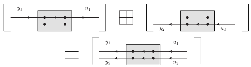
Figure 3: The concatenation of two models $\mathbf{V}_{1}\boxplus\mathbf{V}_{2}$ with the same state space $\mathcal{X}$.

The concatenation sum of two model matrices will result in the type of situation depicted in the picture in figure 2, that is, model (2) with $N_{11}=N_{1},\,N_{22}=N_{2},\,N_{12}=0=N_{21}$.

It is worth remarking that the addition rule (3) makes sense for stochastic flows, either in the Itō or Stratonovich form: here we would have stochastic differential equations

$$dx = v\left(x\right)dt+\sigma\left(x\right)dU$$

$$dY = h\left(x\right)dt+\gamma dU$$

where $U$ is a semi-martingale with $\dot{U}=u$, $\dot{Y}=y$ formally. A concatenation would then take the form

$$dx = \left[v_{1}\left(x\right)+v_{2}\left(x\right)\right]dt+\sigma_{1}\left(x\right)dU_{1}+\sigma_{2}\left(x\right)dU_{2},$$

$$dY_{1} = h_{1}\left(x\right)dt+\gamma_{1}dU_{1},$$

$$dY_{2} = h_{2}\left(x\right)dt+\gamma_{2}dU_{2}.$$

1.4 Series Product

Following this, (assuming the dimensions match) we may then introduce feedback into the concatenated model (4) by setting the output $y_{1}(\cdot)$ of the first system equal to the input $u_{2}(\cdot)$ of the second. Setting $u_{2}=y_{1}(=L_{1}x+N_{1}u_{1})$ and eliminating these as internal signals in the concatenated system above, we reduce to a linear system

$$\left\{\begin{array}[]{l}\dot{x}=\left(K_{1}+K_{2}+M_{2}L_{1}\right)x+\left(M_{1}+M_{2}N_{1}\right)u_{1},\\ y_{2}=\left(L_{2}+N_{2}L_{1}\right)x+N_{2}N_{1}u_{1},\end{array}\right.$$

with model matrix

$$\mathbf{V}_{2}\ast\mathbf{V}_{1}\triangleq\left[\begin{array}[]{cc}K_{1}+M_{2}L_{1}+K_{2}&M_{1}+M_{2}N_{1}\\ L_{2}+N_{2}L_{1}&N_{2}N_{1}\end{array}\right].$$ (5)

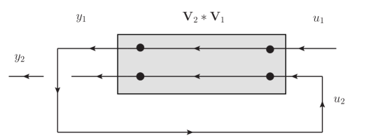
Figure 4: We sketch a concatenation of two models where the output $y_{1}$ is fed back in as input $u_{2}$ to the same system: resulting in a reduced model $\mathbf{V}_{2}\ast\mathbf{V}_{1}$.

We refer to the binary operation $\ast$ as the (general) series product, and this will recur in this paper under various guises.

1.5 The Heisenberg Group

The collection of square model matrices of a fixed dimension, and with lower block $N$ invertible, forms a group with the series product as law. A straightforward representation $\rho$ of these groups as a subgroup of higher dimensional upper block-triangular matrices (with the series product law now replaced by ordinary matrix multiplication) is given by

$$\rho:\left[\begin{array}[]{cc}K&M\\ L&N\end{array}\right]\mapsto\left[\begin{array}[]{ccc}I&M&K\\ 0&N&L\\ 0&0&I\end{array}\right].$$

We now make the observation that we have obtained (in the case $N=I$) the Heisenberg group associated with the canonical commutation relations: we refer to the situation $N\neq I$ as the extended Heisenberg group. For a single-input, single-output, single variable system, we see that the Lie group is generated by

$$\mathfrak{a}=\left[\begin{array}[]{ccc}0&1&0\\ 0&0&0\\ 0&0&0\end{array}\right],\mathfrak{a}^{{\dagger}}=\left[\begin{array}[]{ccc}0&0&0\\ 0&0&1\\ 0&0&0\end{array}\right],\mathfrak{n}=\left[\begin{array}[]{ccc}0&0&0\\ 0&1&0\\ 0&0&0\end{array}\right],\mathfrak{t}=\left[\begin{array}[]{ccc}0&0&1\\ 0&0&0\\ 0&0&0\end{array}\right],$$

and we note the product table

$$\times$$

0 0

0 0

0 0 0 0

0 0 0 0

so that the non-zero Lie brackets are $\left[\mathfrak{a},\mathfrak{a}^{{\dagger}}\right]=\mathfrak{t}$, $\left[\mathfrak{a},\mathfrak{n}\right]=\mathfrak{a}$ and $\left[\mathfrak{n},\mathfrak{a}^{{\dagger}}\right]=\mathfrak{a}^{{\dagger}}$.

1.6 Cascading

We should explain that the terminology of “series” is meant to driving fields acting on a given system in series and the use of the single state variable $x$ allows for the possibility of variable sharing. The situation where two separate systems connected in series will be termed “cascading” and we should emphasize that this is indeed as a special case. Here the joint state $x=\left[\begin{array}[]{c}x_{1}\\ x_{2}\end{array}\right]$ is the direct sum of the states $x_{1}$ and $x_{2}$ of the first and second system respectively, and the cascaded system is then

$$\left[\begin{array}[]{cc}\left[\begin{array}[]{cc}0&0\\ 0&K_{2}\end{array}\right]&\left[\begin{array}[]{c}0\\ M_{2}\end{array}\right]\\ \left[0,L_{2}\right]&N_{2}\end{array}\right]\ast\left[\begin{array}[]{cc}\left[\begin{array}[]{cc}K_{1}&0\\ 0&0\end{array}\right]&\left[\begin{array}[]{c}M_{1}\\ 0\end{array}\right]\\ \left[L_{1},0\right]&N_{1}\end{array}\right]$$

$$=\left[\begin{array}[]{cc}\left[\begin{array}[]{cc}K_{1}&0\\ M_{2}L_{1}&K_{2}\end{array}\right]&\left[\begin{array}[]{c}M_{1}\\ M_{2}L_{1}\end{array}\right]\\ \left[N_{2}L_{1},L_{2}\right]&N_{2}N_{1}\end{array}\right].$$

which gives the correct matrix of coefficients for the systems

$$\mathbf{V}_{1}\equiv\left\{\begin{array}[]{l}\dot{x}_{1}=K_{1}x_{1}+M_{1}u_{1}\\ y_{1}=L_{1}x_{1}+N_{1}u_{1}\end{array}\right.,\quad\mathbf{V}_{2}\equiv\left\{\begin{array}[]{l}\dot{x}_{2}=K_{2}x_{2}+M_{2}u_{2}\\ y_{2}=L_{2}x_{2}+N_{2}u_{2}\end{array}\right.,$$

under the identification $u_{2}=y_{1}$.

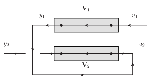
Figure 5: Cascaded systems: a special case of the series product where the inputs $u_{1}$ and $u_{2}$ act on separate state variables, that is, distinct systems.

2 Quantum Stochastic Models

2.1 Second Quantization

We recall the basic ideas of the (Bosonic) second quantization over a separable Hilbert space $\mathfrak{K}$. The Fock space over $\mathfrak{K}$ is $\Gamma\left(\mathfrak{K}\right)=\oplus_{n=0}^{\infty}\left(\otimes_{\text{symm.}}^{n}\mathfrak{K}\right)$, and a total set of vectors is provided by the exponential vectors defined, for test vector $f\in\mathfrak{K}$, by

$$\varepsilon\left(f\right)=1\oplus f\oplus\left(\frac{1}{\sqrt{2!}}f\otimes f\right)\oplus\left(\frac{1}{\sqrt{3!}}f\otimes f\otimes f\right)\oplus\cdots.$$

The creation and annihilation operators with test vector $\phi$ are denoted as $a^{{\dagger}}\left(\phi\right)$ and $a\left(\phi\right)$ respectively, and, along with the differential second quantization $d\Gamma\left(X\right)$ of a self-adjoint operator $X$, they can be defined by

$$a\left(\phi\right)\varepsilon\left(f\right)=\langle\phi|f\rangle\varepsilon\left(f\right),\quad a^{{\dagger}}\left(\phi\right)\varepsilon\left(f\right)=\left.\frac{d}{du}\varepsilon\left(f+u\phi\right)\right|_{u=0},$$

$$d\Gamma\left(X\right)\varepsilon\left(f\right)=\left.\frac{1}{i}\frac{d}{du}\varepsilon\left(e^{iuX}f\right)\right|_{u=0}.$$

The closures of these operators then satisfy the canonical commutation relations (CCR) $\left[a\left(f\right),a^{{\dagger}}\left(g\right)\right]=\langle f|g\rangle$.

Definition 1

Let $\mathfrak{K}$ be a fixed separable Hilbert space. We denote by $U(\mathfrak{K})$ the group of unitary operators on $\mathfrak{K}$ with the strong operator topology. The Euclidean group EU$\left(\mathfrak{K}\right)$ over $\mathfrak{K}$ is the semi-direct product of $U\left(\mathfrak{K}\right)$ with the translation group on $\mathfrak{K}$ and consists of pairs $\left(T,\phi\right)$ where $T\in U(\mathfrak{K})$ and $\phi\in\mathfrak{K}$. The group law is $\left(T_{2},\phi_{2}\right)\circ\left(T_{1},\phi_{1}\right)=\left(T_{2}T_{1},\phi_{2}+T_{2}\phi_{1}\right)$. The extended Heisenberg group over $\mathfrak{K}$ is defined to be

$$\mathfrak{G}\left(\mathfrak{K}\right)=EU\left(\mathfrak{K}\right)\times\mathbb{R}$$

whose basic elements are triples $\left(T,\phi,\theta\right)$ with the group law given by

$$\left(T_{2},\phi_{2},\theta_{2}\right)\vartriangleleft\left(T_{1},\phi_{1},\theta_{1}\right)=\left(T_{2}T_{1},\phi_{2}+T_{2}\phi_{1},\theta_{1}+\theta_{2}+\text{Im}\langle\phi_{2}|T_{2}\phi_{1}\rangle\right).$$ (11)

For $\left(T,\phi\right)\in EU\left(\mathfrak{K}\right)$ we obtain the Weyl unitary $W\left(T,\phi\right)$ on $\Gamma\left(\mathfrak{K}\right)$ defined on the domain of exponential vectors by

$$W\left(T,\phi\right)\,\varepsilon\left(f\right)=\exp\left\{-\frac{1}{2}\left\|\phi\right\|^{2}-\langle\phi|Tf\rangle\right\}\;\varepsilon\left(Tf+\phi\right).$$

The special cases of a pure rotation $\Gamma\left(T\right)=W\left(T,0\right)$, with $\Gamma\left(e^{iX}\right)=e^{id\Gamma\left(X\right)}$, and a pure translation $W\left(\phi\right)=W\left(I,\phi\right)\equiv\exp\left\{a^{{\dagger}}\left(\phi\right)-a\left(\phi\right)\right\}$ lead to the second quantization and the Weyl displacement unitaries respectively. The map $W:$EU$\left(\mathfrak{K}\right)\mapsto U\left(\Gamma\left(\mathfrak{K}\right)\right)$ however yields only a projective unitary representation of the Euclidean group since we have

$$W\left(T_{2},\phi_{2}\right)W\left(T_{1},\phi_{1}\right)=\exp\left\{-i\text{Im}\langle\phi_{2}|T_{2}\phi_{1}\rangle\right\}\;W\left(\left(T_{2},\phi_{2}\right)\circ\left(T_{1},\phi_{1}\right)\right),$$

which is the Weyl form of the CCR and the presence of the multiplier is equivalent to the original CCR.

Proposition 2

A unitary representation of $\mathfrak{G}\left(\mathfrak{K}\right)$ in terms of unitaries on the Bose Fock space $\Gamma\left(\mathfrak{K}\right)$ is then given by the modified Weyl operators $W\left(T,\phi,\theta\right)$ with action

$$W\left(T,\phi,\theta\right)\,\varepsilon\left(f\right)=e^{-i\theta}W\left(T,\phi\right)\,\varepsilon\left(f\right).$$

The role of the “scalar phase” $\theta$ here is of course to absorb the Weyl multiplier.

2.2 Non-abelian Weyl CCR

We now turn to a question, first posed by Hudson and Parthasarathy in 1983 [2], on how to obtain a non-abelian generalization of the Weyl CCR version wherein the role of $U\left(1\right)$ phase is replaced by a (sub-)group of unitaries $U\left(\mathfrak{h}\right)$ over a fixed separable Hilbert space $\mathfrak{h}$. In the present paper we show that the appropriate non-abelian extensions are

$$T\in U\left(\mathfrak{K}\right) \rightleftharpoons S\in U\left(\mathfrak{h}\otimes\mathfrak{K}\right),$$

$$f\in\mathfrak{K} \rightleftharpoons L\in\mathfrak{B}\left(\mathfrak{h},\mathfrak{h}\otimes\mathfrak{K}\right),$$

$$\theta\in\mathbb{R} \rightleftharpoons H\in\mathfrak{B}_{\text{s.a.}}\left(\mathfrak{h}\right),$$

where $\mathfrak{B}_{\text{s.a.}}\left(\mathfrak{h}\right)$ is the set of bounded self-adjoint operators on $\mathfrak{h}$. The corresponding law replacing (11) is the series product:

Definition 3

Let $\mathfrak{h}$ and $\mathfrak{K}$ be a fixed separable Hilbert spaces. The extended Heisenberg group $\mathfrak{G}\left(\mathfrak{h},\mathfrak{K}\right)$ is defined to be the set of triples $\left(S,L,H\right)\in U\left(\mathfrak{h}\otimes\mathfrak{K}\right)\times\mathfrak{B}\left(\mathfrak{h},\mathfrak{h}\otimes\mathfrak{K}\right)\times\mathfrak{B}_{\text{s.a.}}\left(\mathfrak{h}\right)$, with group law given by the (special) series product

$$\left(S_{2},L_{2},H_{2}\right)\vartriangleleft\left(S_{1},L_{1},H_{1}\right)=\left(S_{2}S_{1},L_{2}+S_{2}L_{1},H_{1}+H_{2}+\mathrm{Im}L_{2}^{{\dagger}}S_{2}L_{1}\right).$$ (12)

Unlike the general situation in quantum groups, the product $\vartriangleleft$ does in fact lead to a group law! It originated in the work of one of the authors in relation to a systems theoretic approach to “cascaded” quantum stochastic models [4],[5].

The original answer provided by Hudson and Parthasarathy involved the quantum Itō calculus with initial space $\mathfrak{h}$ and multiplicity space $\mathfrak{K}$, see below, in which a triple $\left(S,L,H\right)$ encoded the information on the coefficients of a quantum stochastic evolution. Apart from a restriction to quantum Itō diffusions $\left(S=I\right)$, they also considered only the operator product of the unitary quantum evolutions which forced the introduction of time dependence - effectively the coefficients $\left(S_{1},L_{1},H_{1}\right)$ will be evolved by the unitary process generated by the second set $\left(S_{2},L_{2},H_{2}\right)$. The $S\neq I$ case is readily handled with the aid of quantum stochastic calculus employing the gauge process.

We shall show that the natural Lie-Trotter product formula for a pair of quantum stochastic evolutions leads naturally to the series product (12), which from the above is the generalization of the Weyl canonical commutations relations to the non-abelian setting.

2.3 Quantum Stochastic Evolutions

We recall the quantum stochastic calculus of Hudson and Parthasarathy [1]. The Hilbert space for the system and noise is $\mathfrak{H}=\mathfrak{h}\otimes\Gamma\left(L_{\mathfrak{K}}^{2}[0,\infty)\right)$ where $\mathfrak{h}$ is a fixed separable Hilbert space called the initial space (modelling a quantum mechanical system) and we have the Fock space over the space of square-integrable $\mathfrak{K}$-valued functions on $[0,\infty)$. Note that $L_{\mathfrak{K}}^{2}[0,\infty)\cong\mathfrak{K}\otimes L^{2}[0,\infty)$. For transparency of presentation, we restrict to the case where $\mathfrak{K}$ is $\mathbb{C}^{n}$, however the general case of a separable Hilbert space presents no difficulties. Let $\left\{e_{j}\right\}_{j=1}^{n}$ be a basis of $\mathfrak{K}$ (the multiplicity space) and define the operators

$$\Lambda^{00}\left(t\right) \triangleq t,$$

$$\Lambda^{i0}\left(t\right) = A_{i}^{{\dagger}}\left(t\right)\triangleq a^{{\dagger}}\left(|e_{i}\rangle\otimes 1_{\left[0,t\right]}\right),$$

$$\Lambda^{0j}\left(t\right) = A_{j}\left(t\right)\triangleq a\left(|e_{j}\rangle\otimes 1_{\left[0,t\right]}\right),$$

$$\Lambda^{ij}\left(t\right) \triangleq d\Gamma\left(|e_{i}\rangle\langle e_{j}|\otimes\chi_{\left[0,t\right]}\right),$$

where $1_{\left[0,t\right]}$ is the characteristic function of the interval $\left[0,t\right]$ and $\chi_{\left[0,t\right]}$ is the operator on $L^{2}[0,\infty)$ corresponding to multiplication by $1_{\left[0,t\right]}$. Hudson and Parthasarathy developed a quantum Itō calculus where integrals of adapted processes with respect to the fundamental processes $\Lambda^{\alpha\beta}$. The Itō table is then

$$d\Lambda^{\alpha\beta}\left(t\right)\,d\Lambda^{\mu\nu}\left(t\right)=\hat{\delta}_{\beta\mu}\,d\Lambda^{\alpha\nu}\left(t\right)$$

where $\hat{\delta}_{\alpha\beta}$ is the Evans-Hudson delta defined to be unity if $\alpha=\beta\in\left\{1,\cdots,n\right\}$ and zero otherwise. This may be written as

$$\times$$

0 0

0 0

0 0 0 0

0 0 0 0

In particular, we have the following theorem [1].

Theorem 4

There exists a unique solution $V\left(\cdot,\cdot\right)$ to the quantum stochastic integro-differential equation

$$V\left(t,s\right)=I+\int_{s}^{t}dG\left(\tau\right)\,V\left(\tau,s\right)$$ (13)

$\left(t\geq s\geq 0\right)$ where

$$dG\left(t\right)=G_{\alpha\beta}\otimes d\Lambda^{\alpha\beta}\left(t\right)$$

with $G_{\alpha\beta}\in\mathfrak{B}\left(\mathfrak{h}\right)$. (We adopt the convention that we sum repeated Greek indices over the range $0,1,\cdots,n$.)

We refer to $\mathbf{G=}\left[G_{\alpha\beta}\right]\in\mathfrak{B}\left(\mathfrak{h}\otimes\left(\mathbb{C}\oplus\mathfrak{K}\right)\right)$, as the coefficient matrix, and $V$ as the left process generated by $\mathbf{G}$. With respect to the decomposition $\mathfrak{h}\otimes\left(\mathbb{C}\oplus\mathfrak{K}\right)=\mathfrak{h}\oplus\left(\mathfrak{h}\otimes\mathfrak{K}\right)$ we may write

$$\mathbf{G}=\left[\begin{array}[]{cc}K&M\\ L&N-I\end{array}\right]$$

where $K\in\mathfrak{B}\left(\mathfrak{h}\right),L\in\mathfrak{B}\left(\mathfrak{h},\mathfrak{h}\otimes\mathfrak{K}\right),M\in\mathfrak{B}\left(\mathfrak{h}\otimes\mathfrak{K},\mathfrak{h}\right)$ and $N\in\mathfrak{B}\left(\mathfrak{h}\otimes\mathfrak{K}\right)$. In the situation where $\mathfrak{K}$ is $\mathbb{C}^{n}$ we have $G_{00}=K$, $L$ is the column vector $\left[G_{i0}\right]$, $M$ is the row vector $\left[G_{0j}\right]$ and $N_{ij}=G_{ij}$.

Adopting the convention that repeated Latin indices are summed over the range $1,\cdots,n$, we may write in more familiar notation [1]

$$dG\left(t\right)=K\otimes dt+M_{i}\otimes dA_{i}\left(t\right)+L_{j}\otimes dA_{j}^{{\dagger}}\left(t\right)+(N_{ij}-\delta_{ij})\otimes d\Lambda_{ij}\left(t\right).$$

For emphasis, we shall often write $V_{\mathbf{G}}\left(\cdot,\cdot\right)$ when we wish to emphasize the dependence on the coefficients $\mathbf{G}$. We remark that the process satisfies the following properties:

1. Flow Law: $V_{\mathbf{G}}\left(t,r\right)V_{\mathbf{G}}\left(r,s\right)=V_{\mathbf{G}}\left(t,s\right)$ whenever $t\geq r\geq s$.

2. Stationarity: $\Gamma\left(\theta_{\tau}\right)V_{\mathbf{G}}\left(t,s\right)\Gamma\left(\theta_{\tau}\right)=V_{\mathbf{G}}\left(t+\tau,s+\tau\right)$ where $\theta_{\tau}$ is the shift map on $L_{\mathfrak{K}}^{2}[0,\infty)$.

3. Localization: with respect to the decomposition $\mathfrak{h}\otimes\Gamma\left(L_{\mathfrak{K}}^{2}[0,\infty)\right)\cong\mathfrak{h}\otimes\Gamma(L_{\mathfrak{K}}^{2}[0,s)\otimes\Gamma\left(L_{\mathfrak{K}}^{2}[s,t)\right)\otimes\Gamma\left(L_{\mathfrak{K}}^{2}[t,\infty)\right)$, $V_{\mathbf{G}}\left(t,s\right)$ acts trivially on the factors $\Gamma(L_{\mathfrak{K}}^{2}[0,s)$ and $\Gamma\left(L_{\mathfrak{K}}^{2}[t,\infty)\right)$.

It is convenient to introduce the projection matrix (the Hudson-Evans delta)

$$\mathbf{\hat{\delta}=}\left[\begin{array}[]{cc}0&0\\ 0&I\end{array}\right]\equiv\left[\hat{\delta}_{\alpha\beta}\right].$$

The key result from [1] is the following concerning unitary evolutions.

Theorem 5

Necessary and sufficient conditions on $\mathbf{G}$ to generate a unitary family are that it satisfies the identities

$$\mathbf{G}+\mathbf{G}^{{\dagger}}+\mathbf{G}^{{\dagger}}\mathbf{\hat{\delta}G}=0\text{ \ \ (isometry), }\mathbf{G}+\mathbf{G}^{{\dagger}}+\mathbf{G\hat{\delta}G}^{{\dagger}}=0\text{ \ \ (co-isometry),}$$

and this is equivalent to $\mathbf{G}$ taking the form

$$\mathbf{G}_{(S,L,H)}=\left[\begin{array}[]{cc}-\frac{1}{2}L^{{\dagger}}L-iH&-L^{{\dagger}}S\\ L&S-I\end{array}\right]$$ (14)

with $S$ is a unitary and $H$ is self-adjoint. We then refer to the triple $\left(S,L,H\right)$ as Hudson-Parthasarathy coefficients.

We shall refer to a coefficient matrix as being a unitary Itō generator matrix if it leads to a unitary process. We may likewise consider right processes, defined as the solution to $U\left(t,s\right)=I+\int_{s}^{t}U\left(\tau,s\right)\,dG\left(\tau\right)$, and denote these as $U_{\mathbf{G}}$. We find that $U_{\mathbf{G}^{{\dagger}}}=V_{\mathbf{G}}^{{\dagger}}$. It turns out that it is technically easier to establish existence of right processes, especially when the $G_{\alpha\beta}$ are unbounded.

2.4 The General Series Product

Definition 6

The (general) series product of two coefficient matrices is defined to be

$$\mathbf{G}_{2}\vartriangleleft\mathbf{G}_{1}\triangleq\mathbf{G}_{1}+\mathbf{G}_{2}+\mathbf{G}_{2}\mathbf{\hat{\delta}G}_{1}.$$ (15)

With respect to the standard decomposition above, this corresponds to

$$\left[\begin{array}[]{cc}K_{2}&M_{2}\\ L_{2}&N_{2}-I\end{array}\right]\vartriangleleft\left[\begin{array}[]{cc}K_{1}&M_{1}\\ L_{1}&N_{1}-I\end{array}\right]=\left[\begin{array}[]{cc}K_{1}+K_{2}+M_{2}L_{1}&M_{1}+M_{2}N_{1}\\ L_{2}+N_{2}L_{1}&N_{2}N_{1}-I\end{array}\right].$$ (16)

The series product is not commutative, however it is readily seen to be associative. Let define the model matrix $\mathbf{V}$ associated to a coefficient matrix $\mathbf{G}$ to be

$$\mathbf{V}\triangleq\mathbf{\hat{\delta}+G}=\left[\begin{array}[]{cc}K&M\\ L&N\end{array}\right].$$

Remark 7

The series product $\mathbf{G}_{2}\vartriangleleft\mathbf{G}_{1}$ for two coefficient matrices implies the corresponding law $\mathbf{V}_{2}\ast\mathbf{V}_{1}$ for the associated model matrices given by

$$\mathbf{V}_{2}\ast\mathbf{V}_{1}=\left[\begin{array}[]{cc}K_{1}+M_{2}L_{1}+K_{2}&M_{1}+M_{2}N_{1}\\ L_{2}+N_{2}L_{1}&N_{2}N_{1}\end{array}\right].$$

Note that this is the natural generalization to the rule (5) already seen for classical linear state based models in series!

Remark 8

For Itō generating matrices for unitary process we have

$$\mathbf{G}_{(S_{2},L_{2},H_{2})}\vartriangleleft\mathbf{G}_{(S_{1},L_{1},H_{1})}=\mathbf{G}_{(S_{2},L_{2},H_{2})\vartriangleleft\left(S_{1},L_{1},H_{1}\right)}$$

which again leads to a unitary process. Therefore the general series product defined in (16) implies the special series product (12).

Lemma 9

The increment $dG$ associated with $V_{\mathbf{G}_{2}\vartriangleleft\mathbf{G}_{1}}\$is related to the increments $dG_{i}$ associated with $V_{\mathbf{G}_{i}}$ through the identity

$$dG=dG_{1}+dG_{2}+dG_{2}dG_{1}$$ (17)

and this is equivalent to the algebraic relation (15) or (16).

This follows from a straightforward application of the quantum Itō calculus.

2.5 The Group of Coefficient Matrices

Definition 10

Denote by GL${}_{\vartriangleleft}\left(\mathfrak{h},\mathfrak{K}\right)$ the subset of $\mathfrak{B}\left(\mathfrak{h}\otimes(\mathbb{C}\oplus\mathfrak{K})\right)$ consisting of operators of the form

$$\mathbf{G}=\left[\begin{array}[]{cc}K&M\\ L&N-I\end{array}\right]$$

with respect to the decomposition $\mathfrak{h}\oplus(\mathfrak{h}\otimes\mathfrak{K})$ of $\mathfrak{h}\otimes(\mathbb{C}\oplus\mathfrak{K})$, and where $N$ is required to be invertible. GL${}_{\vartriangleleft}\left(\mathfrak{h},\mathfrak{K}\right)$ becomes a group under the general series product $\vartriangleleft$ given in (16).

We note that the zero operator is the group identity, and that the series product inverse of $\left[\begin{array}[]{cc}K&M\\ L&N-I\end{array}\right]$ is $\left[\begin{array}[]{cc}-K+MN^{-1}L&-MN^{-1}\\ -N^{-1}L&N^{-1}-I\end{array}\right]$. The extended Heisenberg group $\mathfrak{G}\left(\mathfrak{h},\mathfrak{K}\right)$ is then a subgroup of GL${}_{\vartriangleleft}\left(\mathfrak{h},\mathfrak{K}\right)$ inheriting the series product as law.

The set $\mathfrak{G}\left(\mathfrak{h},\mathfrak{K}\right)$ was introduced in [4] as the collection of all Itō generator matrices (14) and was shown to be a group under the series product (12), though not identified as a Heisenberg group.

Remark 11

The isometry and co-isometry conditions in theorem (5) imply that a two-sided inverse of $\mathbf{G}\sim\left(S,L,H\right)\in\mathfrak{G}\left(\mathfrak{h},\mathfrak{K}\right)$ for the series product is given by $\mathbf{G}^{{\dagger}}\sim\left(S^{{\dagger}},-S^{{\dagger}}L,-H\right)$. The inverse being of course unique.

Lemma 12

The mapping :GL${}_{\vartriangleleft}\left(\mathfrak{h},\mathfrak{K}\right)\mapsto\mathfrak{B}\left(\mathfrak{h}\otimes(\mathbb{C}\oplus\mathfrak{K}\oplus\mathbb{C})\right)$ given by

$$\mathbf{G}=\left[\begin{array}[]{cc}K&M\\ L&N-I\end{array}\right]\mapsto\mathbb{V}_{\mathbf{G}}=\left[\begin{array}[]{ccc}I&M&K\\ 0&N&L\\ 0&0&I\end{array}\right].$$

is an injective group homomorphism.

One readily checks that $\mathbb{V}_{\mathbf{G}_{2}}\mathbb{V}_{\mathbf{G}_{1}}=\mathbb{V}_{\mathbf{G}_{2}\vartriangleleft\mathbf{G}_{1}}$, and $\mathbb{V}_{\mathbf{G}}^{-1}=\mathbb{V}_{\mathbf{G}^{{\dagger}}}$

This representation is the basis for Belavkin’s formalism of quantum stochastic calculus [7],[8]. The Lie algebra of GL${}_{\vartriangleleft}\left(\mathfrak{h},\mathfrak{K}\right)$ (in the Belavkin representation) consists of matrices

$$\mathbb{H}=\left[\begin{array}[]{ccc}0&\mu&\kappa\\ 0&\nu&\lambda\\ 0&0&0\end{array}\right]$$

where now the entries $\kappa,\lambda,\mu,\nu$ are operators and the exponential map is then $\exp\left(\mathbb{H}\right)=\mathbb{V}_{\mathbf{G}}$ with the entries $K,L,M,N$ given by

$$\begin{array}[]{ll}K=\kappa+\mu e_{2}\left(\nu\right)\lambda&M=\mu e_{1}\left(\nu\right),\\ L=e_{1}\left(\nu\right)\lambda,&N=e^{\nu},\end{array}$$ (18)

where we encounter the ‘decapitated exponential’ functions being the entire analytic functions $e_{1}\left(z\right)=\dfrac{e^{z}-1}{z}$, $e_{2}\left(z\right)=\dfrac{e^{z}-1-z}{z^{2}}$.

With an abuse of notation we shall take the Lie algebra of GL${}_{\vartriangleleft}\left(\mathfrak{h},\mathfrak{K}\right)$ to be the vector space $\mathfrak{gl}_{\vartriangleleft}\left(\mathfrak{h},\mathfrak{K}\right)$ of operators $\mathbf{H}=\left[\begin{array}[]{cc}\kappa&\mu\\ \lambda&\nu\end{array}\right]$ with entries matched with the representation element $\mathbb{H}$ above and Lie bracket

$$\left[\mathbf{H}_{2},\mathbf{H}_{1}\right]=\left[\begin{array}[]{cc}\kappa_{2}\lambda_{1}-\kappa_{1}\lambda_{2}&\mu_{2}\nu_{1}-\mu_{1}\xi_{2}\\ \nu_{2}\lambda_{1}-\nu_{1}\lambda_{2}&\left[\nu_{2},\nu_{1}\right]\end{array}\right].$$

With this convention, the exponential map $\widehat{\exp}$ from $\mathfrak{gl}_{\vartriangleleft}\left(\mathfrak{h},\mathfrak{K}\right)$ to GL${}_{\vartriangleleft}\left(\mathfrak{h},\mathfrak{K}\right)$ takes $\mathbf{H}=\left[\begin{array}[]{cc}\kappa&\mu\\ \lambda&\nu\end{array}\right]$ to $\mathbf{G}=\left[\begin{array}[]{cc}K&M\\ L&N-I\end{array}\right]$ with entries given by (18), and this corresponds to

$$\widehat{\exp}\left(\mathbf{H}\right)\triangleq\sum_{n=1}^{\infty}\frac{1}{n!}\mathbf{H}\left(\mathbf{\hat{\delta}H}\right)^{n-1}.$$

The Lie algebra for the subgroup $\mathfrak{G}\left(\mathfrak{h},\mathfrak{K}\right)$ will have elements $\kappa=-i\eta$ and $\nu=-i\sigma$ with $\eta\in\mathfrak{B}_{\text{s.a.}}\left(\mathfrak{h}\right)$ and $\sigma\in\mathfrak{B}_{\text{s.a.}}\left(\mathfrak{h}\otimes\mathfrak{K}\right)$, while $\lambda\in\mathfrak{B}\left(\mathfrak{h},\mathfrak{h}\otimes\mathfrak{K}\right)$ is arbitrary but with $\mu=-\lambda^{{\dagger}}$. The exponential map then leads to the element with Hudson-Parthasarathy parameters

$$\left(S,L,H\right)=\left(e^{-i\sigma},e_{1}\left(-i\sigma\right)\lambda,\eta+\lambda^{{\dagger}}\text{Im}\{e_{2}\left(-i\sigma\right)\}\lambda\right).$$

3 Lie-Trotter Formulas

We set $\Delta^{2}=\left\{\left(t,s\right):t\geq s\geq 0\right\}\subset\mathbb{R}^{2}$, with each element $\left(t,s\right)\in\Delta^{2}$ determining an associated interval $[s,t)$ in $[0,\infty)$. Let $\mathfrak{A}$ be a *-algebra with a fixed topology, which for concreteness we may take as acting on some common domain of a Hilbert space.

Definition 13

Given an $\mathfrak{A}$-valued function $V\left(\cdot,\cdot\right)$ on $\Delta^{2}$ we set

$$\left[V\right]_{\mathcal{P}}\left(t,s\right)\triangleq V\left(t,t_{n}\right)V\left(t_{n},t_{n-1}\right)\cdots V\left(t_{2},t_{1}\right)V\left(t_{1},s\right)$$ (19)

where $\mathcal{P}=\left\{t>t_{n}>t_{n-1}>\cdots>t_{1}>s\right\}$ is a partition of the interval $\left[s,t\right]$. The grid size is $\left|\mathcal{P}\right|=\max_{k}\left(t_{k+1}-t_{k}\right)$ and we say that the limit

$$\lim_{\left|\mathcal{P}\right|\rightarrow 0}\left[V\right]_{\mathcal{P}}\left(t,s\right)$$

exists if $\left[V\right]_{\mathcal{P}}\left(t,s\right)$ converges in the topology to a fixed element of $\mathfrak{A}$ independently of the sequence of partitions used. If the limit is well defined for all $t>s\geq 0$ then we shall write the corresponding two-parameter function as $\lim_{\left|\mathcal{P}\right|\rightarrow 0}\left[V\right]_{\mathcal{P}}\left(\cdot,\cdot\right)$.

3.1 Examples

3.1.1 Trivial

If we start with a quantum stochastic exponential $V=V_{\mathbf{G}}$, the flow property implies that we trivially have $\left[V_{\mathbf{G}}\right]_{\mathcal{P}}\left(t,s\right)=V_{\mathbf{G}}\left(t,s\right)$ for any partition $\mathcal{P}$.

3.1.2 Quantum stochastic exponentials

In the setting of quantum stochastic calculus, we let $G\left(t\right)=G_{\alpha\beta}\otimes\Lambda^{\alpha\beta}\left(t\right)$, with $G_{\alpha\beta}$ bounded, and set $\left(I+\Delta G\right)\left(t,s\right)=I+G\left(t\right)-G\left(s\right)$, then

$$V_{\mathbf{G}}=\lim_{\left|\mathcal{P}\right|\rightarrow 0}\left[1+\Delta G\right]_{\mathcal{P}}.$$

3.1.3 Holevo’s time-ordered exponentials

In the same setting, we let $H\left(t\right)=H_{\alpha\beta}\otimes\Lambda^{\alpha\beta}\left(t\right)$ and set $e^{\Delta H}\left(t,s\right)=e^{H\left(t\right)-H\left(s\right)}$ then the limit is the Holevo time-ordered exponential [6]

$$\,Y_{\mathbf{H}}=\lim_{\left|\mathcal{P}\right|\rightarrow 0}\left[e^{\Delta H}\right]_{\mathcal{P}},$$

often written as $\,Y_{\mathbf{H}}\left(t,s\right)=\overleftarrow{\exp}\int_{s}^{t}dH\left(\tau\right)$. Holevo established strong convergence for such limits, including an extension to the situation where $H\left(t\right)=\int_{0}^{t}H_{\alpha\beta}\left(\tau\right)\otimes d\Lambda^{\alpha\beta}\left(\tau\right)$ with $H_{\alpha\beta}\left(\cdot\right)\,$strongly continuous $\mathfrak{B}\left(\mathfrak{h}\right)$-valued functions with the $H_{i0}\left(\cdot\right)$ and $H_{0j}\left(\cdot\right)$ square integrable, and the $H_{ij}\left(\cdot\right)$ integrable.

We should think of the $\mathbf{H=}\left[H_{\alpha\beta}\right]$ of the Holevo time-ordered exponential as an element of the Lie algebra $\mathfrak{gl}_{\vartriangleleft}\left(\mathfrak{h},\mathfrak{K}\right)$. In particular, we have the following result.

Lemma 14

The Holevo time-ordered exponential $\,Y_{\mathbf{H}}$ is equivalent to the quantum stochastic exponential $V_{\mathbf{G}}$ where $\mathbf{G}=\widehat{\exp}\left(\mathbf{H}\right)$.

Proof. We observe that the integro-differential equation (13) can be given the infinitesimal form

$$V_{\mathbf{G}}\left(t+dt,t\right)=I+dG\left(t\right)$$

while for the time-ordered exponential we have

$$\,Y_{\mathbf{H}}\left(t+dt,t\right)=e^{dH\left(t\right)}.$$

For the two to be equal, we need the coefficients of

$$dG\left(t\right)=dH\left(t\right)+\frac{1}{2!}dH\left(t\right)dH\left(t\right)+\cdots$$

to coincide, but from the Itō table this implies $\mathbf{G}=\widehat{\exp}\left(\mathbf{H}\right)$.   

3.2 The Quantum Stochastic Lie-Trotter Formula

Definition 15

Given $\mathfrak{A}$-valued functions $V_{1}\left(\cdot,\cdot\right)$ and $V_{2}\left(\cdot,\cdot\right)$ on $\Delta^{2}$, we define their product $V_{2}\cdot V_{1}$ interval-wise, that is

$$\left(V_{2}\cdot V_{1}\right)\left(t,s\right)\triangleq V_{2}\left(t,s\right)V_{1}\left(t,s\right).$$ (20)

Note that the product $V_{2}\cdot V_{1}$ will not generally satisfy the flow property even when $V_{1}$ and $V_{2}$ do, with the result the limit $\lim_{\left|\mathcal{P}\right|\rightarrow 0}\left[V_{2}\cdot V_{1}\right]_{\mathcal{P}}\left(t,s\right)$ may now not be trivial.

As an example, take the algebra of $n\times n$ matrices $\mathfrak{A}=M_{n}\left(\mathbb{C}\right)$ and define $U_{A}\left(t,s\right)=e^{\left(t-s\right)A}$, then the Lie product formula $\lim_{n\rightarrow\infty}\left(e^{tA/n}e^{tB/n}\right)^{n}=e^{t\left(A+B\right)}$ can be recast in the form

$$\lim_{\left|\mathcal{P}\right|\rightarrow 0}\left[U_{A}\cdot U_{B}\right]_{\mathcal{P}}=U_{A+B}.$$

The extension to the algebra of operators over a Hilbert space with strong operator topology was subsequently given by Trotter. For instance, if $A=-iH_{1}$ and $B=-iH_{2}$ where $H_{1}$ and $H_{2}$ are self-adjoint with $H_{1}+H_{2}$ essentially self-adjoint on the overlap of their domains then the strong limit exists (Theorem VIII.31 [11]). The case of strongly continuous contractive semigroups on Banach spaces is given as Theorem X.5.1 in [12].

We are now able to formulate our main result.

Theorem 16

Let $\mathbf{G}_{1}$ and $\mathbf{G}_{2}$ be a pair of bounded coefficient matrices on the same Hudson-Parthasarathy space, then in the strong operator topology

$$\lim_{\left|\mathcal{P}\right|\rightarrow 0}\left[V_{\mathbf{G}_{2}}\cdot V_{\mathbf{G}_{1}}\right]_{\mathcal{P}}=V_{\mathbf{G}_{2}\vartriangleleft\mathbf{G}_{1}}.$$ (21)

Similarly we find $\lim_{\left|\mathcal{P}\right|\rightarrow 0}\left[V_{\mathbf{G}_{m}}\cdot\ldots\cdot V_{\mathbf{G}_{2}}\cdot V_{\mathbf{G}_{1}}\right]_{\mathcal{P}}=V_{\mathbf{G}_{m}\vartriangleleft\cdots\vartriangleleft\mathbf{G}_{2}\vartriangleleft\mathbf{G}_{1}}$, where the interval-wise multiple products are defined in the obvious way.

Proof. To see where this comes from, we note from the infinitesimal form that $V=\lim_{\left|\mathcal{P}\right|\rightarrow 0}\left[V_{\mathbf{G}_{2}}\cdot V_{\mathbf{G}_{1}}\right]_{\mathcal{P}}$ should satisfy the analogous equation

$$V\left(t+dt,t\right)=\left(I+dG_{2}\left(t\right)\right)\left(I+dG_{1}\left(t\right)\right)\equiv I+dG\left(t\right)$$

where $dG=dG_{1}+dG_{2}+dG_{2}dG_{1}$, but by (17) we recognize this as just the infinitesimal generator of $V_{\mathbf{G}_{2}\vartriangleleft\mathbf{G}_{1}}$. In contrast to the traditional Lie-Trotter formulas, the above limit depends on the order of $V_{\mathbf{G}_{2}}\cdot V_{\mathbf{G}_{1}}$ and is therefore asymmetric under interchange of $V_{\mathbf{G}_{2}}$ and $V_{\mathbf{G}_{1}}$.   

3.3 Special Cases

3.3.1 Lie-Trotter formula

The special case $\mathbf{G}_{i}=\left[\begin{array}[]{cc}K_{i}&0\\ 0&0\end{array}\right]$ recovers the usual Lie-Trotter formulas.

3.3.2 Separate Channels

Let $\mathbf{G}_{i}=\left[\begin{array}[]{cc}K_{i}&M_{i}\\ L_{i}&N_{i}-I\end{array}\right]$ be coefficient matrices with common initial space $\mathfrak{h}$ but different multiplicity spaces $\mathfrak{K}_{i}$. We combine the multiplicity space into a single space $\mathfrak{K}=\mathfrak{K}_{1}\oplus\mathfrak{K}_{2}$ and ampliate both coefficient matrices as follows:

$$\mathbf{\tilde{G}}_{1}=\left[\begin{array}[]{ccc}K_{1}&M_{1}&0\\ L_{1}&N_{1}-I_{1}&0\\ 0&0&0\end{array}\right],\mathbf{\tilde{G}}_{2}=\left[\begin{array}[]{ccc}K_{2}&0&M_{2}\\ 0&0&0\\ L_{2}&0&N_{2}-I_{2}\end{array}\right]$$

then

$$\mathbf{\tilde{G}}_{2}\vartriangleleft\mathbf{\tilde{G}}_{1}=\left[\begin{array}[]{ccc}K_{1}+K_{2}&M_{1}&M_{2}\\ L_{1}&N_{1}-I_{1}&0\\ L_{2}&0&N_{2}-I_{2}\end{array}\right].$$

The right hand side is taken as the definition of the concatenation $\mathbf{G}_{1}\boxplus\mathbf{G}_{2}$ of the two separate coefficient matrices: this is consistent with the definition of concatenation introduced earlier for model matrices. Theorem (16) then implies that

$$\lim_{\left|\mathcal{P}\right|\rightarrow 0}\left[V_{\mathbf{\tilde{G}}_{2}}\cdot V_{\mathbf{\tilde{G}}_{1}}\right]_{\mathcal{P}}=V_{\mathbf{G}_{2}\boxplus\mathbf{G}_{1}}.$$

This is equivalent to the result derived by Lindsay and Sinha [3]. We should also mention the recent work of Das, Goswami and Sinha indicates that the Trotter formula should also hold at the level of flows [13].

Acknowledgement: The authors are grateful to Professor Kalyan Sinha for presenting his work on quantum stochastic Lie-Trotter formula [3] during a visit to Aberystwyth within the framework of the UK-India Education and Research Initiative.

References

- [1] [1] R.L. Hudson and K.R. Parthasarathy, Quantum Ito’s formula and stochastic evolutions, Commun. Math. Phys. 93, 301-323 (1984)
- [2] [2] R.L. Hudson and K.R. Parthasarathy, Generalized Weyl operators, in Stochastic Analysis and Applications, Lecture Notes in Mathematics 1095, Ed. A. Truman, D. Williams, Springer (1983)
- [3] [3] J.M. Lindsay, K.B. Sinha, A quantum stochastic Lie-Trotter product formula, Indian J. Pure Appl. Math., 41(1):313-325, February (2010)
- [4] [4] J. Gough, M.R. James, Quantum Feedback Networks: Hamiltonian Formul- ation, Commun. Math. Phys. 287, 1109-1132 (2009)
- [5] [5] J. Gough, M.R. James, The series product and its application to feedforward and feedback networks, IEEE Trans. Autom. Control 54, 2530 (2009)
- [6] [6] A.S. Holevo, Time-ordered exponentials in quantum stochastic calculus, Quantum Probability and Related Topics, Vol. VII, 175-202 (1992)
- [7] [7] V.P. Belavkin: On quantum Ito algebras and their decompositions, Letters in Mathematical Physics 45, 131-145 (1998)
- [8] [8] O.G. Smolyanov, A. Truman, The Gough-James model of quantum feedback networks in the Belavkin representation, (Russian) Dokl. Akad. Nauk 435, no. 5, 591-594 (2010)
- [9] [9] K.R. Parthasarathy, An Introduction to Quantum Stochastic Calculus, Birkhauser, Berlin, (1992)
- [10] [10] M.P. Evans, R.L. Hudson, Multidimensional quantum diffusions, Springer LNM 1303, 69-88 (1988)
- [11] [11] M. Reed and B. Simon, Methods of Modern Mathematical Physics I: Functional Analysis, Academic Press, New York (1975)
- [12] [12] M. Reed and B. Simon, Methods of Modern Mathematical Physics II: Analysis of Operators, Academic Press, New York (1975)
- [13] [13] B. Das, D. Goswami and K.B. Sinha, A Trotter product formula for quantum stochastic flows arXiv:1001.0233v1