Optical bistability in one dimensional doped photonic crystals
with spontaneously generated coherence

Abstract

We investigate optical bistability in a multilayer one-dimensional photonic crystal where the central layer is doped with $\Lambda$-type three level atoms. We take into account the influence of spontaneously generated coherence when the lower atomic levels are sufficiently close to each other, in which case Kerr-type nonlinear response of the atoms is enhanced. We calculate the propagation of a probe beam in the defect mode window using numerical nonlinear transfer matrix method. We find that Rabi frequency of a control field acting on the defect layer and the detuning of the probe field from the atomic resonance can be used to control the size and contrast of the hysteresis loop and the threshold of the optical bistability. In particular we find that, at the optimal spontaneously generated coherence, three orders of magnitude lower threshold can be achieved relative to the case without the coherence.

I Introduction

Optical bistability (OB) is a striking manifestation of nonlinear behavior in an optical system where two separate stationary output states are possible for a given input Gibbs (1985); Abraham and Smith (1982). Technologically, this fundamental nonlinear phenomenon is used for all-optical logic and memory operations Soljačić et al. (2002); Barclay et al. (2005). Modern applications demand more compact, more noise tolerant, and faster OB based devices that can operate under lower power thresholds over a wide range of multistability.

Nonlinear photonic crystal (PC) systems Scalora et al. (1994); Danckaert et al. (1991); Agranovich et al. (1991) are microphotonic devices, such as photonic switches Mingaleev and Kivshar (2002); Yanik et al. (2003a); Mingaleev et al. (2006), diodes Tocci et al. (1995); Zhao et al. (2006); Xue et al. (2010), or transistors Solja?i? et al. (2003); Yanik et al. (2003b), which offer sub-picosecond operation times at miliwatt power levels and suitability for large scale optical integration Bravo-Abad et al. (2007). They can be tailored for efficient optical switching by using embedded atoms in PCs Guo and Lü (2009); John and Quang (1996, 1997); Ma and John (2011); Takeda and John (2011); Vujic and John (2007). Conventional OB in PCs utilizes dynamic shifting of the band edge while the doped PCs allow for dispersive OB via dynamic shifting of the defect mode Wang et al. (1997). One-dimensional multilayer PC (1DPC) systems Lidorikis et al. (1997); Wang et al. (1997); Novitsky and Mikhnevich (2008) are considered for controlling OB. Adding extra coating layers Gupta and Agarwal (1987), phase matching layer He and Cada (1992), negative index layer Jose (2009), or subwavelenght layers Hou et al. (2008) next to the nonlinear one were proposed to control OB. Doping 1DPC Wang et al. (1997) was suggested as a compact alternative to such strategies which require increasing the size of the system.

Effects of the microscopical details and possible quantum coherence of the atomic structure are not taken into account in the general discussion of controlling OB in doped 1DPCs. On the other hand effect of atomic coherence on OB has been studied in three level atoms Walls and Zoller (1980); Walls et al. (1981); Harshawardhan and Agarwal (1996); Antón and Calderón (2002); Antón et al. (2003); Wang and Xu (2009); and it is found that spontaneously generated coherence (SGC) effect Javanainen (1992) strongly enhances the nonlinear response of three level atoms Niu and Gong (2006). The effect of SGC is due to a counterintuitive role played by the vacuum modes. When two low lying levels are separated less than the excited state line width, same vacuum modes can be emitted and re-absorbed so that quantum decay trajectories interfere to establish quantum coherence for the lower levels. This intrinsically nonlinear effect contributes to enhancement of the nonlinear response. Our objective is to utilize this fact for efficient control of OB in doped 1DPCs.

We consider a 1DPC with $\Lambda$-type three level atoms embedded in the central layer. Utilizing spontaneously generated coherence which enhances Kerr-type nonlinearity of the atoms in the central layer, we find that such a system allows for wide range control of the contrast in optical switching and the level of power threshold. Our idea exploits first the enhancement of local intensity of light by the defect modes of the dopant atoms in the central layer of the PC, and second it exploits the additional enhancement of nonlinear response of the atoms by SGC. Both the enhanced intensity and nonlinear response are translated into three orders of magnitude lowering of threshold power to reach OB regime incontrast to the case without SGC. In addition our proposal brings flexibility to control of hysteresis loop, contrast and threshold of OB compactly via the atomic parameters such as detuning and Rabi frequencies. In particular high contrast between bistable transmission states is found for a certain set of atomic parameters. Significant recent technological progress to introduce dopants Braun et al. (2006) or quantum dots Kuroda et al. (2008) in PCs makes our proposal promising for next generation photonic diodes and transistors to realize all-optical logic and memory applications. Alternatively quantum dots Dutt et al. (2005), semiconductor heterostructures Wu et al. (2005b) or equivalent dressed state schemes Wu et al. (2005a) can be considered for possible implementations of our proposal.

The paper is organized as follows. In Sec. II, we describe our model and the method of calculation. The multilayer 1DPC system doped with $\Lambda$-type three level atoms in the central layer is described by presenting the level scheme, SGC, linear and nonlinear susceptibilites Niu and Gong (2006) in Sec. II.1. The nonlinear transfer matrix method Gupta and Agarwal (1987); Jiang et al. (2003) we employ to calculate the probe transmission is introduced in Sec. II.2. The results are discussed in Sec. III, where the transmission coefficient for various atomic parameters is discussed. Possible implementation schemes of our model is discussed at the end of this section. We conclude in Sec. IV.

II Light Transmission through 1D PC containing a doped layer of $\Lambda$-Type three level atoms with SGC

II.1 Model System

We consider a 1DPC as depicted in Fig. 1 which is a symmetric multilayer stack $(AB)_{2}AD(AB)_{2}A$ where $A,B$ and $D$ are of thickness $d_{A},d_{B}$ and $d_{D}$. All the layers are linear dielectrics with refractive indices $n_{A},n_{B}$ and $n_{D}$. We take $n_{A}=2.22$ and $n_{D}=n_{B}=1.41$ as in Ref. Steinberg et al. (1993). The parameters are related to the midgap (central) wavelength $\lambda_{\text{pc}}=692$ nm of the PC by $n_{A}d_{A}=n_{B}d_{B}=\lambda_{\text{pc}}/4$ and $n_{D}d_{D}=\lambda_{pc}/2$.

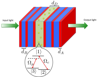
Figure 1: Schematic of the 1DPC we consider. It is a symmetric multilayer stack $(AB)_{2}AD(AB)_{2}A$ where $A,B$ and $D$ are of thickness $d_{A},d_{B}$ and $d_{D}$. The central layer is doped with $\Lambda$-type three-level atoms. The coupling field drives the transitions between the levels $|1\rangle$ and $|2\rangle$with the Rabi frequency $\Omega_{c}$, and the probe field drives the transitions between the levels $|1\rangle$ and $|3\rangle$ with the Rabi frequency $\Omega_{p}$. We assume the coupling field is directly applied onto the doped layer $D$ while the probe field is transmitted from the left of the 1DPC by the normal incident input field. The output is collected from right of the 1DPC structure.

The central (defect) layer is doped with $N$ $\Lambda$-type three level atoms. A resonant coupling field is directly applied to the defect layer and drives the transition between the states $|1\rangle$ and $|2\rangle$ with the Rabi frequency $\Omega_{c}$. The normal incident field to the left of the 1DPC structure arrives to the defect layer and drives the transition between the states $|1\rangle$ and $|3\rangle$ as the probe field with the Rabi frequency $\Omega_{p}$. The modified spontaneous emission rates of the atoms inside the PC are assumed to be $2\gamma_{2}$ and $2\gamma_{3}$ from the excited state $|1\rangle$ to the lower states $|2\rangle$ and $|3\rangle$, respectively.

We assume that the lower levels are closely spaced so that the two transitions to the excited state interact with the same vacuum mode and hence SGC is present. The first ($\chi^{(1)}$) and third-order ($\chi^{(3)}$) susceptibilities of such $\Lambda$-type three-level atoms with SGC atoms are given by Niu and Gong (2006)

$$\chi^{(1)} = -\frac{2N|\mu_{13}|^{2}}{\varepsilon_{0}\hbar}\frac{\Delta_{p}}{\Omega_{c}^{2}+\text{i}(\gamma_{2}+\gamma_{3}+\text{i}\Delta_{p})\Delta_{p}},$$ (1)

$$\begin{split}\chi^{(3)}&=\frac{2N|\mu_{13}|^{4}}{3\varepsilon_{0}\hbar^{3}}(4i\Omega_{c}^{4}p^{2}\gamma_{2}(\gamma_{2}+\gamma_{3})\Delta_{p}^{2}(\Omega_{c}^{2}-\Delta_{p}^{2})\\ &+\Delta_{p}[\Omega_{c}^{2}+\text{i}(\gamma_{2}+\gamma_{3}+i\Delta_{p})\Delta_{p}]\\ &\times[\Omega_{c}^{2}-\text{i}(\gamma_{2}+\gamma_{3}-i\Delta_{p})\Delta_{p}]\\ &\times\{2\Omega_{c}^{4}\gamma_{3}-\text{i}\Omega_{c}^{2}\gamma_{2}(\gamma_{2}+\gamma_{3})\Delta_{p}\\ &+\Delta_{p}^{2}[3\Omega_{c}^{2}\gamma_{2}+\gamma_{2}\gamma_{3}^{2}+\gamma_{2}^{3}\\ &+2\gamma_{3}(\Omega_{c}^{2}+\gamma_{2}^{2})]\})/\beta,\end{split}$$ (2)

with

$$\begin{split}\beta&=\gamma_{3}[\Omega_{c}^{3}-\text{i}\Omega_{c}(\gamma_{2}+\gamma_{3}-i\Delta_{p})\Delta_{p}]^{2}\\ &\times[\Omega_{c}^{2}+\text{i}(\gamma_{2}+\gamma_{3}+i\Delta_{p})\Delta_{p}]^{3}.\end{split}$$ (3)

where $\triangle_{p}=\omega_{13}-\omega_{p}$ is the detuning of the probe field frequency $\omega_{p}$ from the atomic transition resonance at $\omega_{13}$ between the levels $|1\rangle$ and $|3\rangle$. The Rabi frequencies $\Omega_{c}$ and $\Omega_{p}$ are constrained as $\Omega_{c(p)}=\Omega_{c(p)}^{0}\sin\theta=\Omega_{c(p)}^{0}\sqrt{1-p^{2}}$ where $p=\cos\theta=\vec{\mu}_{12}.\vec{\mu}_{13}/|\vec{\mu}_{12}.\vec{\mu}_{13}|$ is defined as the SGC parameter for the two dipole moments $\vec{\mu}_{12}$ and $\vec{\mu}_{13}$ making an angle $\theta$ with each other. We distinguish the Rabi frequency for the transverse aligned dipoles ($\theta=90^{\circ}$) as $\Omega_{c(p)}^{0}$. The constraint arises by the requirement that the probe and the coupling fields do not interact with each other’s transitions so that one must be perpendicular to the dipole moment coupled to the other. In general Rabi frequencies are complex numbers but we shall take them real valued here for simplicity. Mathematically the relative phase between the probe and the coupling fields can be studied by considering a complex valued SGC parameter and may lead to multistability beyond OB. We shall not include this case to our considerations.

II.2 Nonlinear transfer matrix method

We employ the standard characteristic (transfer) matrix method to calculate the transmission coefficient for our 1DPC system Gupta and Agarwal (1987); Agarwal and Gupta (1987); Gupta and Ray (1988). The transfer matrix $M$ for the multilayer structure in Fig. 1 is written by

$$M =(M_{A}M_{B})^{2}M_{A}M_{D}(M_{A}M_{B})^{2}M_{A},$$ (4)

where $M_{j}$ with $j=A,B,D$ are the transfer matrices for the corresponding layers. The transmission coefficient $T$ is the ratio of the transmitted field intensity to the incident field intensity and it is related to the elements $m_{ij}$ with $i,j=1,2$ of the transfer matrix $M$ by

$$T =\left|\frac{2n_{0}}{(m_{11}+m_{12}n_{0})+(m_{21}+m_{22}n_{0})}\right|,$$ (5)

where $n_{0}$ is the refractive index of the air. We assume the input field is incident from the air and the output field is transmitted into the air.

When a TE-polarized normal incident pulse is considered, transfer matrix for the defect layer $D$, doped with nonlinear atoms, is given by Gupta and Agarwal (1987); Gupta (1989)

$$M_{D}=\left(\begin{array}[]{cc}m_{11}^{(d)}&m_{12}^{(d)}\\ m_{21}^{(d)}&m_{22}^{(d)},\end{array}\right)$$ (8)

where

$$m_{11}^{(d)} =\frac{1}{k_{+}+k_{-}}\left(k_{-}\text{e}^{-\text{i}k_{+}d_{D}}+k_{+}\text{e}^{\text{i}k_{-}d_{D}}\right),$$ (9)

$$m_{12}^{(d)} =\frac{k_{0}}{k_{+}+k_{-}}\left(\text{e}^{-\text{i}k_{+}d_{D}}-\text{e}^{\text{i}k_{-}d_{D}}\right),$$ (10)

$$m_{21}^{(d)} =\frac{k_{-}k_{+}}{k_{0}(k_{+}+k_{-})}\left(\text{e}^{-\text{i}k_{+}d_{D}}-\text{e}^{\text{i}k_{-}d_{D}}\right),$$ (11)

$$m_{22}^{(d)} =\frac{1}{k_{+}+k_{-}}\left(k_{+}\text{e}^{-\text{i}k_{+}d_{D}}+k_{-}\text{e}^{\text{i}k_{-}d_{D}}\right).$$ (12)

Here the propagation constants of the forward and backward propagating probe field inside the doped layer $D$ are denoted by $k_{+}$ and $k_{-}$ and they depend on the field amplitudes due to the nonlinear dopant atoms by

$$k_{\pm}=k_{0}n_{l}(1+U_{\pm}+2U_{\mp})^{\frac{1}{2}},$$ (13)

where $k_{0}$ is the wave vector in vacuum, and

$$U_{\pm} =\chi^{(3)}|A_{\pm}|^{2},$$ (14)

where $A_{j\pm}$ and $A_{j\pm}$ are the amplitudes of the forward and backward propagating probe fields and $n_{l}$ is the linear refractive index of the layer $D$ including the dopant atoms. Dielectric permittivity of defect layer $(\epsilon)$ can be written in the form of $\epsilon=\epsilon_{l}+\chi^{(3)}|E(z)|^{2}$ with $\epsilon_{l}$ is the linear dielectric permittivity. For our system (a linear defect layer doped with $\Lambda$-type three level atoms) linear dielectric permittivity can be calculated by

$$\epsilon_{l}=\epsilon_{D}+\chi^{(1)}.$$ (15)

Here $\epsilon_{D}=n_{D}^{2}$ is dielectric permittivity of linear defect layer.

Nonlinear character of the dopant atoms makes the wave vectors $k_{\pm}$ depend on the forward and backward propagating probe field intensities $U_{\pm}$ inside the central layer. In order to construct $M_{D}$ we need to determine $U_{\pm}$ by solving a set of coupled nonlinear equations,

$$U_{\pm}=\left|\frac{p_{+}(m_{11}^{(r)}+m_{12}^{(r)})\pm(m_{21}^{(r)}+m_{22}^{(r)})}{p_{-}+p_{+}}\right|^{2}U_{f},$$ (16)

with

$$p_{\pm}=n_{l}\sqrt{1+U_{\mp}+2U_{\pm}}$$ (17)

for a given transmitted intensity $U_{f}$ (scaled by $\chi^{(3)}$) by the fixed point iteration method Gupta and Agarwal (1987). Here we denote the elements of the transmission matrix for the multilayer stack to the right of the central layer, $M_{r}=(M_{A}M_{B})^{2}M_{A}$ as $m_{ij}^{(r)}$. These equations reflect the relation between the tangential field components at the right boundary of the central layer and at the output surface of the 1DPC.

For the layers $A$ and $B$, the transfer matrices $M_{A}$ and $M_{B}$ are given by Jiang et al. (2003),

$$M_{j} =\left(\begin{array}[]{cc}\cos(k_{j}d_{j})&-\text{i}\frac{\sqrt{\mu_{j}}}{\sqrt{\epsilon_{j}}}\sin(k_{j}d_{j})\\ -\text{i}\frac{\sqrt{\epsilon_{j}}}{\sqrt{\mu_{j}}}\sin(k_{j}d_{j})&\cos(k_{j}d_{j})\end{array}\right),$$ (20)

where $k_{j}=\sqrt{\epsilon_{j}\mu_{j}}\omega_{p}/c$ with $j=A,B$. Using the relation between the incident intensity $U_{\text{i}}$ (scaled by $\chi^{(3)}$) and the transmitted intensity $U_{f}$ by $U_{i}=U_{f}/T$ we determine the dependence of the transmission to the $U_{i}$.

As the relations among the intensities $U_{\pm},U_{f}$ and $U_{i}$ are scaled by the nonlinear susceptibility $\chi^{(3)}$, the explicit dependence of the transfer matrix to the atomic parameters are only due to the linear index $n_{l}$. To control OB efficiently both the linear and nonlinear susceptibilities hence should be carefully considered together. In the next section we numerically evaluate the transmission coefficient to reveal the effects of atomic parameters and SGC on the OB in the light of the linear and nonlinear responses of the dopant atoms.

III Results and Discussion

Our purpose is to examine the influence of atomic parameters, specifically the probe detuning, coupling field Rabi frequency, and the SGC parameter, on the OB. For that aim it is convenient for us to write the expressions of the linear and nonlinear susceptibilities in forms that explicitly depends on these parameters per se. We take equal decay rates from the excited state to the closely spaced doublet, $\gamma_{2}=\gamma_{3}:=\gamma$, for simplicity and divide the numerators and denominators of Eq. (1) and Eq. (2) by $\gamma$ and $\gamma^{13}$, respectively.

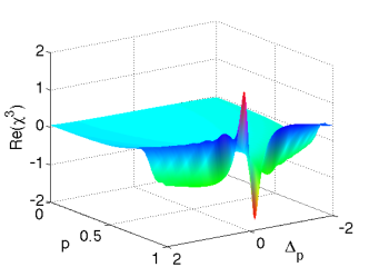
Figure 2: (Color online) Dependence of the real part of the nonlinear susceptibility $\text{Re}(\chi^{3})$ (in arbitrary units (a. u.)) on the SGC parameter $p$ and the probe detuning $\Delta_{p}$ for $\Omega_{c}^{0}=4$. Significant enhancement of the nonlinear response of the system can be obtained at the optimal value of $p\sim 1$.($\Delta_{p}$ and $\Omega_{c}^{0}$ are dimensionless and scaled by the spontaneous decay rate $\gamma$.)

We use $\gamma$ to scale quantities in frequency units, especially $\Omega_{c},\Delta_{p}$, and to make them dimensionless, so that we can write $\chi^{(1)}=s^{(1)}\tilde{\chi}^{(1)}$ and $\chi^{(3)}=s^{(3)}\tilde{\chi}^{(3)}$ where the factors $s^{(1)},s^{(3)}$

$$s^{(1)}=\frac{2N|{\mu_{13}|^{2}}}{\varepsilon_{0}\hbar\gamma},\quad s^{(3)}=\frac{2N|\mu_{13}|^{4}}{3\varepsilon_{0}\hbar^{3}\gamma^{3}},$$ (21)

depending on the atomic constants are separated from the dimensionless factors $\tilde{\chi}^{(1)},\tilde{\chi}^{(3)}$

$$\tilde{\chi}^{(1)} = -\frac{\Delta_{p}}{\Omega_{c}^{2}+\text{i}(2+\text{i}\Delta_{p})\Delta_{p}},$$ (22)

$$\tilde{\chi}^{(3)} = (8i\Omega_{c}^{4}p^{2}\Delta_{p}^{2}(\Omega_{c}^{2}-\Delta_{p}^{2})$$ (23)

$$+ \Delta_{p}[\Omega_{c}^{2}+\text{i}(2+i\Delta_{p})\Delta_{p}]$$ (24)

$$\times [\Omega_{c}^{2}-\text{i}(2-i\Delta_{p})\Delta_{p}]\times\{2\Omega_{c}^{4}-\text{i}2\Omega_{c}^{2}\Delta_{p}$$ (25)

$$+ \Delta_{p}^{2}[3\Omega_{c}^{2}+2+2(\Omega_{c}^{2}+1)]\})/\tilde{\beta},$$ (26)

with

$$\tilde{\beta} = [\Omega_{c}^{3}-\text{i}\Omega_{c}(2-i\Delta_{p})\Delta_{p}]^{2}$$ (27)

$$\times [\Omega_{c}^{2}+\text{i}(2+i\Delta_{p})\Delta_{p}]^{3},$$ (28)

depending on the control parameters. Using the relation between the dipole moment and the decay rate $\gamma=|{\mu_{13}|^{2}}\omega_{13}^{3}/3\pi\varepsilon_{0}\hbar c^{3}$, it can be verified immediately that $s^{(1)}=6\pi Nc^{3}/\omega_{13}^{3}$ is dimensionless while $s^{(3)}=s^{(1)}\pi\varepsilon_{0}c^{3}/\omega_{13}^{3}\hbar\gamma$ has units of inverse electric field squared.

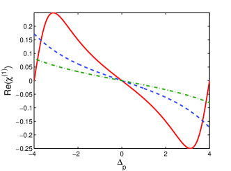
(a)

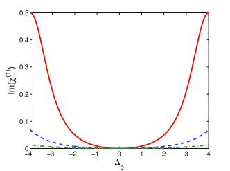
(b)

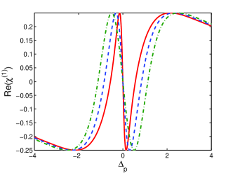
(c)

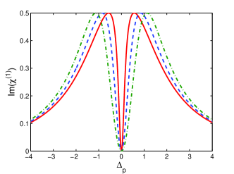
(d)

Figure 3: (Color online) (a) Real $\text{Re}\chi^{(1)}$ and (b) imaginary $\text{Im}\chi^{(1)}$ parts of the linear susceptibility as a function of probe detuning $\Delta_{p}$ when SGC is absent ($p=0$). (c) Real $\text{Re}\chi^{(1)}$ and (d) imaginary $\text{Im}\chi^{(1)}$ parts of the linear susceptibility as a function of probe detuning $\Delta_{p}$ when SGC is present ($p=0.99$). Curves with red solid line, blue dashed line, and green dash-dotted line correspond to the $\Omega_{c}^{0}=4,\Omega_{c}^{0}=6$, and $\Omega_{c}^{0}=8$, respectively. ($\Delta_{p}$ and $\Omega_{c}^{0}$ are dimensionless and scaled by the spontaneous decay rate $\gamma$.)

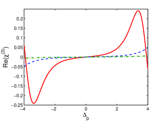
(a)

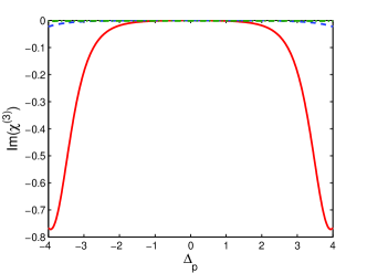
(b)

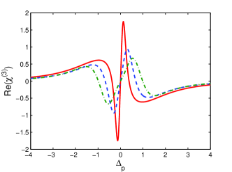
(c)

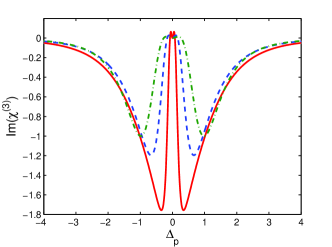
(d)

Figure 4: (Color online) (a) Real $\text{Re}\chi^{(3)}$ and (b) imaginary $\text{Im}\chi^{(3)}$ parts of the nonlinear susceptibility (dimensionless) as a function of probe detuning $\Delta_{p}$ when SGC is absent ($p=0$). (c) Real $\text{Re}\chi^{(3)}$ and (d) imaginary $\text{Im}\chi^{(3)}$ parts of the nonlinear susceptibility (dimensionless) as a function of probe detuning $\Delta_{p}$ when SGC is present ($p=0.99$). Curves with red solid line, blue dashed line, and green dash-dotted line correspond to the $\Omega_{c}^{0}=4,\Omega_{c}^{0}=6$, and $\Omega_{c}^{0}=8$, respectively. ($\Delta_{p}$ and $\Omega_{c}^{0}$ are dimensionless and scaled by the spontaneous decay rate $\gamma$.)

We apply the nonlinear transfer matrix method to determine the transmission of an incident probe light with carrier frequency $\omega_{p}=2.5\times 10^{15}$ Hz near to the midgap frequency $\omega_{pc}=2\pi c/\lambda_{pc}=2.72\times 10^{15}$ Hz of the 1DPC. Doped 1DPC supports a linear defect mode around the midgap frequency and allows for a linear transmission window within the band gap. In order to make nonlinear response relevant for the probe transmission we consider the following scheme. The atomic resonance is assumed to be slightly detuned from the probe and thus lies within the photonic band gap but just below the transmission window opened by the linear defect mode. The atomic spontaneous decay rate would then be modified Bravo-Abad et al. (2007) but we do not need its actual value as we use it for scaling factor. Typical range of values for the control parameters we use in our simulations relative to $\gamma$ are as follows. Detuning of the incident light from the atomic probe transition is assumed to be in the range from $\Delta_{p}=0.05$ to $\Delta_{p}=0.15$. Control field Rabi frequency $\Omega_{c}^{0}$ is considered to be in the range $\Omega_{c}^{0}\sim 1-10$. We also assume background material as air surrounding the non-magnetic dielectric layers so that $n_{0}=1,\mu_{A,B,D}=1$.

While we use $\chi^{(3)}$ when we investigate the transmission as a function of the incident field intensity $I_{i}$; it only indirectly appears in the treatment of nonlinear transfer matrix method, as a scaling factor within $U_{\pm}$ in Eq. (14). The linear susceptibility however is directly and explicitly used in the calculations. Due to these two distinct stages of using $\chi^{(1)}$ and $\chi^{(3)}$, we drop the factor $s^{(3)}$ in $\chi^{(3)}$ by assuming the intensity is measured in arbitrary units (a.u.). In the following we shall drop the tilde notation and use $\chi^{(3)}$ in place of $\tilde{\chi}^{(3)}$. We further assume that $s^{(1)}=1$, which can be satisfied by taking a proper $N$. In our case $\omega_{13}\sim 10^{15}$ Hz so that $N\lesssim 10^{20}$ m^-3. For the same parameters $s^{(3)}\sim 5.4\times 10^{-8}$ m²/V². Intensity can be converted from a.u. to physical units of mW$/$cm² for these atomic variables by a multiplication factor of $50$. Despite this theoretical association of a.u. with the physical units here, we follow the common conventional wisdom to give intensity in a.u. due to its specific measurement dependence.

We first examine the behavior of $\chi^{(3)}$ to determine the optimal set of parameters to get significant nonlinear response out of the doped 1DPC system. Enhancement of the nonlinearity by the SGC can be seen in Fig. 2 where the largest value of $\chi^{(3)}$ is found at $\Delta_{p}\sim 0.05$ for $p\sim 1$. Such a large nonlinear response can be exploited for OB if the absorption is weak in the corresponding frequency window.

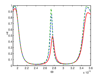
Figure 5: (Color online) Linear transmission coefficient $T$ of a 1DPC including a central defect layer doped with $\Lambda$-type three level atoms with SGC as a function of the incident field frequency $\omega$ (in Hz) for $\Omega_{c}^{0}=4$ (blue dashed curve), $\Omega_{c}^{0}=6$ (green dash-dotted curve) and $\Omega_{c}^{0}=8$ (red solid curve). Other parameters are $\Delta_{p}=0.05$ and $p=0.99$. ($\Delta_{p}$ and $\Omega_{c}^{0}$ are dimensionless and scaled by the spontaneous decay rate $\gamma$.)

We subsequently explore the linear susceptibility and absorption properties of the system in Fig. 3 and in Fig. 4 where we compare the cases of lack of SGC ($p=0$) and presence of optimal ($p=0.99$) SGC. These figures also explore the effect of the coupling laser Rabi frequency. The curves with the red solid line, blue dashed line and the green dash-dotted line correspond to $\Omega_{c}^{0}=4,\Omega_{c}^{0}=6$, and $\Omega_{c}^{0}=8$, respectively.

Real part of the linear susceptibility exhibits steep negative dispersion near the probe resonance if SGC is present, as can be seen by comparing Fig. 3a with Fig. 3c. This is consistent with the superluminal light propagation and the Hartman effect which are enhanced by the SGC according to recent investigations of 1DPC doped with $\Lambda$-type three level atoms Sahrai and Esfahlani (2013). Barrier length independence of the tunneling time MacColl (1932), known as the Hartman effect Hartman (1962), in the doping region can be beneficial for OB based fast optical switching applications for practical implementation of our model system. When we investigate the imaginary part of the linear susceptibility in Fig. 3b and in Fig. 3d, we see that the transmission window becomes more narrow in the presence of SGC. Nevertheless, strong nonlinearity regime, in particular around the optimal detuning of $\Delta_{p}\sim 0.05$, remains in the narrow transmission window. The negative dispersion gets steeper and the width of the transmission window gets smaller with the decrease of the $\Omega_{c}^{0}$.

These conclusions hold true when we consider the nonlinear dispersion and absorption curves in Fig. 4. Real part of the nonlinear susceptibility plotted in Fig. 4a and in Fig. 4c show that the steep changes around the probe resonance emerge in the presence of SGC. In contrast to anomalous linear dispersion, nonlinear one is normal with positive slope. More crucial observation for the ease of OB operation is the significant enhancement of the magnitude of $\chi^{(3)}$ with the SGC. About an order of magnitude increase is obtained at $p=0.99$. The nonlinear transmission window is narrowed as well. The detuning required for the strong nonlinear response is within the narrow window of transmission. An additional information to similar Fig. 2 available here is the effect of $\Omega_{c}^{0}$. The nonlinear dispersion gets steeper and the nonlinear transmission window gets narrower with the decrease of $\Omega_{c}^{0}$. Accordingly these observations suggest that we can make a further optimal choice for large nonlinear response in a transmission window by taking $\Omega_{c}^{0}=4$ at $\Delta_{p}=0.05$.

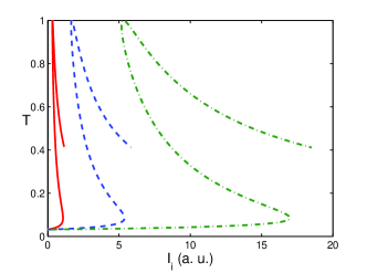
(a)

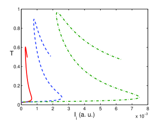
(b)

Figure 6: (Color online) Transmission coefficient $T$ of a 1DPC including a central defect layer doped with $\Lambda$-type three level atoms with SGC as a function of the incident light intensity $I_{i}$ (in arbitrary units (a.u.)) at probe detuning $\Delta_{p}=0.05$ when (a) SGC is absent ($p=0$) and when (b) SGC is optimal ($p=0.99$). Different curves with red solid line, blue dashed line, and green dash-dotted line correspond to the $\Omega_{c}^{0}=4,\Omega_{c}^{0}=6$, and $\Omega_{c}^{0}=8$, respectively. ($\Delta_{p}$ and $\Omega_{c}^{0}$ are dimensionless and scaled by the spontaneous decay rate $\gamma$.)

If we calculate the linear transmission spectrum (by taking $\chi^{(3)}=0$) we can notice the emergence of the defect mode within the photonic band gap. The result, for different values of Rabi frequencies of the control field, is plotted in Fig. 5. The transmission resonances become narrower for smaller $\Omega_{c}^{0}$. It is expected that it is easier to achieve OB with sharp defect modes  Agarwal and Gupta (1986). Typical solution to achieve such narrow Airy resonances in Fabry-Perot type systems is to enlarge the number of coupled resonators or photonic crystal coatings Gupta and Agarwal (1987). Our atomic control parameter $\Omega_{c}^{0}$ could potentially be a more compact solution than increasing the layers in the 1DPC. On the other hand the effect of $\Omega_{c}^{0}$ on OB is not trivial. In addition to its influence on the width of the defect mode, an accompanying frequency shift of the defect mode from the probe frequency can also be seen in the Fig. 5. It is known that high frequency shift of the linear defect mode yields higher OB threshold Wang et al. (1997). The width of the defect mode becomes sharper while its frequency shifts higher away from the probe resonance with the decrease of $\Omega_{c}^{0}$. In our case therefore beneficial and harmful effects of $\Omega_{c}^{0}$ on OB compete. We need to investigate the nonlinear transmission carefully to assess the net effect of $\Omega_{c}^{0}$ explicitly.

Including the full linear and nonlinear response, the transmission coefficient $T$ is calculated and plotted as a function of the input field intensity $I_{i}$ (in arbitrary units (a.u.)) for different Rabi frequencies $\Omega_{c}^{0}$ of the coupling field in Fig. 6. We see that by decreasing the Rabi frequency of coupling field $\Omega_{c}^{0}$ the threshold of the OB is decreased. Comparison of Fig. 6a and Fig. 6b shows that SGC significantly lowers the OB threshold while keeping the hysteresis loop size the same. Three orders of magnitude decrease in the threshold intensity can be achieved. Maximum transmission or the contrast between the lowest and highest points in the hysteresis loop is decreased with the increasing SGC. This effect is stronger fow smaller $\Omega_{c}^{0}$. An optimal choice of the Rabi frequency of the coupling field and the SGC parameter can be made depending on the requirements of particular applications.

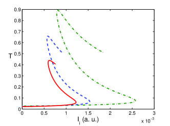
Figure 7: (Color online) Transmission coefficient $T$ of a 1DPC including a central defect layer doped with $\Lambda$-type three level atoms with SGC as a function of the incident light intensity $I_{i}$ (in arbitrary units (a.u.)) at coupling field Rabi frequency $\Omega_{c}^{0}=6$ and when SGC is optimal ($p=0.99$). Different curves with blue dashed line, green dash-dotted line and red solid line correspond to the $\Delta_{p}=0.05,\Delta_{p}=0.1$, and $\Delta_{p}=0.15$, respectively. ($\Delta_{p}$ and $\Omega_{c}^{0}$ are dimensionless and scaled by the spontaneous decay rate $\gamma$.)

Nonlinear transfer matrix method produces the relation between $T$ and scaled dimensionless incident field intensity $U_{i}$. We used the expression $I_{i}=c\varepsilon_{0}U_{i}/2\mathrm{Re}(\chi^{(3)})$ for the incident field intensity to plot the Figs. 6-7. Dependence of $\chi^{(1)}$ on the SGC parameter $p$ and $\Omega_{c}^{0}$ via $\Omega_{c}$ results in differences in the values of $U_{i}$ at the OB threshold. These differences are further changed by $\chi^{(3)}$ when $U_{i}$ is translated to the physical intensity $I_{i}$. A comparison of $\chi^{(1)}$, $\chi^{(3)}$ and $U_{i}$ can be made by examination of Table 1 which confirms the results in Figs. 6a-6b. In particular, we see that linear susceptibilities are close to $0$ and only slightly different from each other when there is no SGC, so that threshold values of $U_{i}$ are not distinguishable for $\Omega_{c}=4,6,8$. However, differences in nonlinear susceptibility even in this case lead to reasonably distinct values of threshold intensity for OB. When SGC is present both the $U_{i}$ and $I_{i}$ threshold values are well distinguishable for $\Omega_{c}=4,6,8$.

Table 1: List of linear $\chi^{(1)}$ and nonlinear $\chi^{(3)}$ susceptibilities, and the corresponding probe intensity $U_{i}$ at the threshold of OB for probe detuning $\Delta_{p}=0.05$, SGC parameter $p=0.99$, and coupling field Rabi frequencies $\Omega_{c}^{0}=4,6,8$. All the parameters are scaled and dimensionless as explained in the text.

p	$\Omega_{c}^{0}$	$\mathrm{Re}(\chi^{(1)})$	$\mathrm{Re}(\chi^{(3)})$	$U_{i}$
$0$	$4$	$-0.0031$	$0.00039$	$0.31$
$0$	$6$	$-0.0014$	$0.000077$	$0.31$
$0$	$8$	$-0.0008$	$0.000024$	$0.31$
$0.99$	$4$	$-0.1439$	$0.9756$	$0.48$
$0.99$	$6$	$-0.0687$	$0.1969$	$0.38$
$0.99$	$8$	$-0.0391$	$0.0621$	$0.34$

In Fig. 7 the effect of atomic detuning on the threshold value of OB is investigated. It can be seen that this atomic parameter can also be used for controlling of OB in the system. The threshold of OB decreases by decreasing the atomic detuning for a given $\Omega_{c}^{0}$ at the cost of lower contrast between the highest and lowest transmission outputs.

We conclude this section with a brief discussion of implementation of our model in a real physical system. Observation of SGC in real atoms, despite some controversial experimental claims, is too difficult due to the stringent requirement of finding closely lying levels with parallel dipole moments. More flexibility for implementing advantages of SGC can be achieved by designing equivalent dressed state representations Wu et al. (2005a). Quantum coherence of a bare state system can be mapped to SGC of dressed state picture which corresponds to quasi degenerate low lying levels required for SGC. On the other hand SGC has already been observed with artificial atoms such as charged quantum dots Dutt et al. (2005). Embedding GaAs quantum dot structures in photonic crystals Kuroda et al. (2008) is an avaliable techonology which can be tailored to implement our model system. Semiconductor quantum well heterostructures can also be used in place of the defect layer in our system. Quantum coherence in the resonant tunneling can replace the SGC effect equivalently Wu et al. (2005b). Due to the Hartmann effect the size of the heterostructures should not influence the speed of the OB operation. The overall increase of the size of the multilayer system would be comparable to the doped defect layer as the quantum well heterostructure consists of few thin nanometer size layers. Surrounding PC layers (A,B in Fig. 1) are about $50-80$ nm each typically.

IV Conclusions

We explored the effects of spontaneously generated coherence and atomic control parameters, specifically probe detuning and control field Rabi frequency, on the characteristics of optical bistability in a 1DPC doped with $\Lambda$-type three-level atoms. It is found that OB threshold, size of the hysteresis loop, and the contrast between OB outputs can be controlled over significantly wide ranges by these parameters. We find the parameter regimes which allow for negligible absorption and enhanced nonlinear response simultaneously. We discussed that the proposed model system can be implemented effectively using artificial atoms such as charged quantum dot heterostructures. Doped multilayer photonic crystals with engineered quantum coherence offer more compact solutions to flexible wide range control in photonic switching applications than present alternatives based upon coupled systems or systems with large number of layers.