Analysis of multichannel measurements of rare processes
with uncertain expected background and acceptance

Abstract

A typical experiment in high energy physics is considered. The result of the experiment is assumed to be a histogram consisting of bins or channels with numbers of corresponding registered events. The expected background and expected signal shape or acceptance are measured in separate auxiliary experiments, or calculated by the Monte Carlo method with finite sample size, and hence with finite precision. An especially complex situation occurs when the expected background in some of the channels happens to be zero due to either a fluctuation of the auxiliary measurement (or simulation) or because it is truly zero. Different statistical methods give different confidence intervals for the full signal rate and different significances of the signal$+$background hypothesis versus the pure background hypothesis. Detailed analysis and numerical tests are presented.

1 Introduction

Rates of rare processes in high energy physics have sometimes to be estimated from a few observed events. This can happen during the research of very rare processes or at the beginning of any research. Reconstruction of such rates is a complex and ambiguous problem [1], especially in the presence of uncertain nuisance parameters.

1.1 Typical experiment

The result of an experiment is frequently represented by a histogram consisting of several, $k$, bins or channels, $k\geq 1$. Each of these channels keeps the number of events $n_{i}$ registered in this channel, where $i$ is the channel number. The number $n_{i}$ is sampled from the Poisson distribution with a parameter, which is unique for each channel. Events in each channel are expected to be produced by background processes, called background, and by a studied process called a signal, all distributed according to the Poisson law. The expected background $b_{i}$ and expected signal (shape) or acceptance $a_{i}$ (we prefer the term “expected signal” and omit the word “shape” for briefness and because we do not require $a_{i}$ to be normalized, c.f. Refs. [2, 3]) are either known exactly or measured in separate auxiliary experiments, or calculated by the Monte Carlo method with finite sample sizes, and hence with a finite precision. In the general case these nuisance parameters can correspond to different exposures or luminosities, so the expected full rate in the main experiment is expressed by

$$f_{i}=t_{a}a_{i}s+t_{b}b_{i}\,,$$ (1)

or in the vector notation

$$\vec{f}=t_{a}\vec{a}\,s+t_{b}\vec{b}\,,$$ (2)

where $t_{a}$ and $t_{b}$ are the ratios of exposures of the main and respective auxiliary experiments and $s$ is the real signal rate, the absolute value, or the value relative to the expected signal rate.

We consider here only the stochastic uncertainties of $a_{i}$ and $b_{i}$. The uncertainties that are presumably non-stochastic can usually be assumed stochastic in some more general sense and can be handled by similar methods. Both $a_{i}$ and $b_{i}$ are assumed to be “measured” in the respective “auxiliary experiments” as the numbers $n_{ai}$ and $n_{bi}$ sampled from the Poisson distributions with the corresponding parameters $a_{i}$ or $b_{i}$.

The purpose of the experimental research is to determine the most probable full signal rate, a confidence interval for it, and the significance of the signal (plus background) hypothesis versus the pure background hypothesis.

1.2 Zero channels of expected background

An especially challenging situation arises when the expected background in some of the channels happens to be zero in the auxiliary background experiment due to either a fluctuation of the auxiliary measurement or because it is truly zero. Such a situation can happen in the search of very rare processes in experiments with very good background rejection. For such experiments it is difficult to perform the Monte Carlo simulation of background with large final statistics (i.e. to obtain a large number of background events passed through all triggers, reconstructions, “cuts”, and selections), because in order to do this one needs to run huge initial statistics. Hence it is not possible to distinguish the cases of a downward background fluctuation and the true zero background on the basis of existing information. It is then unclear both conceptually and numerically, how to interpret a non-zero result of the main experiment in this channel.

Literature does not offer any recipe for dealing with zeros in the expected background.

One could simply ignore such channels. Or zeros can be removed by unification or smoothing of neighboring or presumably similar channels, some of which are non-zero. The similarity of the channels is typically indicated by neighboring values of a response variable produced by multivariate analysis methods. But any zero-removing procedure can lead, briefly speaking, to an unexpected change of the precision and complicates its estimation. The most doubtful case is when a few zero channels appear in the distribution of the expected background by the response variable at the end of the distribution, where the expected background is minimal and the expected signal is maximal. When the expected-background spectrum finishes with several zero bins and there is nothing to the right-hand side of them, any interpolation or smoothing is ambiguous. In this case, the end of the spectra, which has to be the most important region for the results, is subjected to effectively arbitrary treatment.

Therefore, it is interesting to investigate which statistical methods, if any, provide correct results in such problems, when the channels’ content is taken as is, without forbidding of zeros or smoothing.

1.3 Tests of intervals

The idea is to generate a sequence of pseudo-experiments with some small enough true background, to divide the experimental results into different numbers of channels, to treat them by all available statistical methods, and to compare the results. In particular, it is interesting to see whether an optimal number of channels can be chosen on the basis of the data available for the experimenter, for instance, by minimizing the interval width reconstructed by the data of the single experiment (not the average width). We will study a rough optimization with selection of the best division from several divisions with different numbers of channels incremented by a factor of 1.5–3: 1, 2, 3, 5, 10, 30. Channels in each division have the same width by the response variable.

If the obtained interval for the searched parameter includes (“covers”) its true value, whatever it is, with the stated probability, or frequency in a long sequence of experiments, it is said that the coverage is provided. Then, from the formal classical viewpoint the method is acceptable. The coverage probability is usually allowed to be greater than stated. In this case the coverage is called “conservative”. Nuisance parameters are assumed to have some true values in this sequence too. During the analysis they are unknown, but they do not need to be reconstructed or “covered”. This is effectively a “frequentist” or a “classical” viewpoint. Both terms are accepted, see, for example, Ref. [1], §26.1 of Ref. [4], and Ref. [5]. The intervals obtained by the minimization of width mentioned above or by other methods of the binning selection and calculated with different binning for each given experiment can also be tested this way and can be accepted, if they provide the stated coverage probability.

Such an investigation is interesting not only in the context of the problem with zeros, but in a much wider context. Many statistical methods provide accurate coverage for the problems with known expected signal and background, but do not guarantee it for the problems with nuisance parameters. The Bayesian method and the profile likelihood (or likelihood ratio) method do not guarantee frequentist coverage for samples of finite sizes [1], but it is interesting to see whether they provide it in practice. If the parameter of interest is restricted, typically to be non-negative, some classical methods can produce empty or unphysically small intervals in the case of a downward fluctuation of background and small true signal (c.f. Refs. [6, 7]). Some test statistics allow one to obtain finite intervals by maximizing the upper limit and minimizing the lower limit with respect to nuisance parameters or by the projection of the confidence set to the parameter of interest. However, these procedures can require unrealistic computing resources in the case of many nuisance parameters, the optimal values of the latter can be incompatible with measurements, and the resulting interval can reportedly “badly over-cover”[8]. Another issue which is discussed in the literature is the coverage of the upper border of the classical intervals for the experiments microscopically dependent on the signal [9].

Frequentist tests reported in Refs. [10, 11, 12, 13] do not include some interesting methods and cases, such as, in particular, zeros in the expected background.

1.4 Tests of significance

The notion of coverage does not exist in the case of significance. We can only calculate the significance itself in a different way, for example, with different test statistic and (or) for different sample or subset of experiments. For example, the uniformity of a $p$-value distribution is sometimes tested [14, 15, 16]. Denoting the estimate of the $p$-value by $\rho$ (in order to distinguish it from the probability density, which is denoted by $p$ herein) and its probability density distribution by $p(\rho)$ one can check whether $\int_{0}^{\rho_{t}}p(\rho)\,\mathrm{d}\rho\leq\rho_{t}$ for any small enough threshold $\rho_{t}$. If the sign is “$<$”, this is the conservative case, better than assumed to be necessary. The opposite case “$>$” is considered as a signature of overestimated significance, see a discussion in Section 1.3 of Ref. [16]. The equality means that the $p$-value is uniform. If $\rho$ is discrete, we imply here that the equality occurs for $\rho_{t}$ equal to all possible $\rho$. The integral in this inequality can be considered as a $p$-value for the test statistic $\rho_{t}$ or for the correspoding significance, assuming that the small values of $\rho_{t}$ or large values of the correspoding significance indicate disagreement with the null hypothesis. This alternative $p$-value can differ from the regular $\rho_{t}$, if nuisance parameters are involved. The uniformity of the alternative $p$-value can be tested in the same way. Alternative $p$-values are always uniform for the sample of experiments, for which the corresponding regular $p$-values are calculated (the latter can be calculated internally with completely different pseudo-experiments, depending on the method), but the regular $p$-values are not necessarily uniform for this sample. For some methods there exist samples for which regular $p$-values are equal to alternative $p$-values and both are uniform (see Section 4.2.1). Intuitively, the statistical analysis by such methods is more reliable.

The particular case of the one-channel “on/off” problem solved through the test of the ratio of Poisson means [14] yields the significance that appears to be independent of the background hypothesis, though dependent on the total $n_{\mathrm{on}}+n_{\mathrm{off}}$ measurement. There is no similar simplification known for the many-channel case.

As with the confidence limits, the significance calculated with certain test statistics can have a non-zero minimum at some values of nuisance parameters [15]. But these values are sometimes incompatible with their measurements [17], and it is very difficult to find this minimum in the case of many nuisance parameters. If the nuisance parameters are constrained by their confidence limits with an arbitrary confidence level $\beta$ [17], the sum of the obtained maximal $p$-value and $\beta$ can be used as the $p$-value for the test statistic which is this very sum. This $p$-value is uniform or conservative, but it depends on arbitrary $\beta$ and can exaggerate the significance of a particular experiment, if the true nuisance parameters are outside the confidence limits. Finally, it is not easy to calculate the confidence limits for many correlated parameters.

1.5 Content

This paper is organized as follows. In the next section the test problem is described in more detail. The optimization of division (binning) is briefly outlined.

The following main groups of methods are described and tested in the following sections:

• The Bayesian approach (Section 3) [1, 2, 18, 19, 20, 21, 22] with new “safe” priors and new modification of the central intervals.

• The frequentist treatment of the maximum likelihood estimate (Section 4) without nuisance parameters [7, 23] and many new methods of their inclusion.

• The profile likelihood or the likelihood ratio method (Section 5) — currently both notations are used in the literature, see Refs. [1, 12, 18].

• The frequentist treatment of likelihood ratios or the $CL_{s}$ methods (Section 6) [9, 24, 25, 26, 27] with different denominators and various old and new ways of nuisance parameters inclusion.

Features of confidence intervals are illustrated by many plots. Characteristics of significance obtained by each appropriate method despite the computational difficulties are briefly described. A comparison of significance obtained by different methods for particular simple cases is given in Section 7.

Conclusions are presented in the last section.

2 The test problem

2.1 Notations

The conditional probability (density) of obtaining an experimental result $x$ at given parameter $y$ is denoted by $P(x|y)$ for the discrete case and by $p(x|y)$ for the continuous case, except for the Bayesian prior distributions, which are denoted by $\pi(x)$. All $P$, $p$, and $\pi$ denote probabilities (densities for $p$ and $\pi$) of observing corresponding values, but not functions with a fixed form. We retain the same notations even when we consider them as functions of $y$ and call them“likelihoods” (§8.22 of Ref. [30] and Ref. [1]).

Then, for instance, the joint probability of obtaining $n_{i}$ events in the $i$-th channel of the main experiment, $n_{ai}$ in the auxiliary signal experiment, and $n_{bi}$ in the auxiliary background experiment is denoted by

$$P(n_{i}, n_{ai},n_{bi}|s,a_{i},b_{i})=$$

$$P(n_{i}|s,a_{i},b_{i})P(n_{ai}|a_{i})P(n_{bi}|b_{i})=$$

$$P(n_{i}|t_{a}a_{i}s+t_{b}b_{i})P(n_{ai}|a_{i})P(n_{bi}|b_{i}).$$ (3)

If all channels are involved, the corresponding multiplication of probabilities is denoted, for short, by

$$\prod_{i}P(n_{i},n_{ai},n_{bi}| s,a_{i},b_{i})=P(\vec{n},\vec{n}_{a},\vec{n}_{b}|s,\vec{a},\vec{b})=$$

$$P(\vec{n}|t_{a}\vec{a}\ s+t_{b}\vec{b})P(\vec{n}_{a}|\vec{a})P(\vec{n}_{b}|\vec{b}).$$ (4)

The elementary probabilities $P(n|\mu)$ of observing $n$ events with the average expectation $\mu$ for this work are assumed to follow the Poisson law:

$$P(n|\mu)=\mathrm{Poisson}(n,\mu)=\frac{\mu^{n}e^{-\mu}}{n!}\,.$$ (5)

2.2 Parameters and algorithm

For most of the calculations in this paper it is assumed that the multivariate response variable, denoted $x$, varies from 0 to 1. This interval is equally divided into $k$ bins with step $1/k$ and end points $x_{i}$, $x_{i+1}$. The true background and signal distributions are

$$f_{b}(x)=Ce^{-qx}, f_{a}(x)=Ce^{-q(1-x)}$$

respectively, where $q\geq 1$ and the normalization factor $C=q/(1-e^{-q})$ is needed to make the integral equal to unity. The true parameters $a_{i}$ and $b_{i}$ are determined by equalities:

$$a_{i}=N_{a}\displaystyle\int\limits_{x_{i}}^{x_{i+1}}f_{a}(x)\,\mathrm{d}x\,,\ \ b_{i}=N_{b}\displaystyle\int\limits_{x_{i}}^{x_{i+1}}f_{b}(x)\,\mathrm{d}x\,,$$ (6)

where $N_{a}$ and $N_{b}$ are the mean total numbers of detected events in the corresponding auxiliary experiments.

In order to generate the auxiliary pseudo-experiments one can either generate the numbers of actual signal events by the Poisson law with the mean $N_{a}$ and similarly for the background events with $N_{b}$ and distribute these events randomly according to Eqs. (6), or generate the numbers in each bin by the Poisson law according to the means given by Eqs. (6). Two separate histograms, one with expected signal and the other with expected background, are filled for each pair of auxiliary pseudo-experiments. If the case of exactly known parameters is considered, the corresponding histograms can be filled by $a_{i}$ or $b_{i}$ or both, depending on the case. Similarly in the simulated main pseudo-experiment the events are generated in either of two ways taking into account Eqs. (6) and Eq. (1) with $s=s_{\mathrm{true}}$, the true signal rate, which is unknown for the analysis program and has to be reconstructed by it. To obtain identical events with a different number of channels only the histograms with the largest number of channels are filled by the method described above. The other ones are obtained by summing up the content of the neighboring channels. For tests of intervals we consider divisions with 1, 2, 3, 5, 10 and 30 channels. This is all done in a separate “main” program. For each division the main program calls the analysis program and transmits to the latter three histograms: the “main” and two “auxiliaries”. The analysis program knows $t_{a}$ and $t_{b}$ and reconstructs the confidence interval for $s$, its most probable value, and the significance.

After the end of the loop by divisions for each “event” (that is for each main and auxiliary experiments) the main program can compare the intervals obtained for each division and choose the best according to any criteria. After the end of the loop by experiments it can check the coverage of these intervals. The significance is tested differently.

Most of the calculations of intervals for this work were made with $t_{a}=0.25$, $N_{a}=100$, $t_{b}=5$, $N_{b}=50$, $s_{\mathrm{true}}=2$, and $q=3$. The behavior of many methods was also tested at microscopic dependence on signal in the conditions of $t_{a}=0.25/20$, as well as for the zero true signal $s_{\mathrm{true}}=0$ with normal dependence on it ($t_{a}=0.25$). The significance was also studied for many other configurations.

With such parameters the probability of observing zeros in the expected background is very high for many-channel cases. For just the last channel the probability of observing no events in it is around 12% for the 5-channel case, 40% for the 10-channel case and 76% for the 30-channel case.

Most of the tests of intervals were performed in this paper for the one-sided confidence level of 90%. In some cases, especially for the cases without uncertainties, which are typically calculated very quickly, the levels of 99% and even 99.845% ($3\sigma$ level) were tested.

2.3 Optimization of division

The most basic method of optimization is finding the division (binning) that provides the minimal interval width. This should usually be combined with some additional conditions, such as the absence of zeros in the expected-signal distribution, or another condition, depending on the method. The mentioned condition effectively excludes too many-channel divisions from consideration. The optimization by separate limits usually results in the insufficient coverage probability for any method. If the coverage for fixed divisions is 90%, usually something like 80% is obtained by this optimization.

In the case with nuisance parameter uncertainties the minimization of the interval width usually reduces the coverage with respect to the minimal coverage obtained at fixed divisions. Thus, if there is no noticeable margin in the latter, the coverage of the intervals optimized by widths can be slightly less than required.

We will not consider here various other ways of optimization that can eventually mix a channel with true zero expected background with a neighboring non-zero channel, thus potentially reducing the sensitivity of the experiment.

A simple way to provide the claimed optimized coverage is to request better fixed-division coverage. Then it needs to know for how much it should be better. In general this is an unclear issue.

A better way of improving the optimized coverage of any non-Bayesian method, when the optimal divisions are obtained by the minimization of the interval width, is the use of the Bayesian credible intervals for finding the optimal division and presenting the interval obtained by the non-Bayesian method for this division. Optimization by a different interval-finding method, in a simplistic explanation, chooses the interval which is not always the shortest for a given method, thus improving the optimized coverage of the given method. This optimization should not necessarily mix the zero-background channel with others. This method with modified (see Section 3.6) Bayesian credible intervals is used throughout this work.

If for particular conditions the lower limit is close to zero or almost always zero, it can be non-informative for the purpose of division optimization. In particular, this can happen if the confidence required is very large, for example 99.9% for the test example studied in this work. The optimization by width is then reduced to the optimization by the upper limit and one can predict the lack of coverage as if optimized by the single upper limit. If the problem is caused by the extremely high confidence level, the optimization can be performed by the intervals obtained with a smaller level. Otherwise it is assumed, though not tested, that another criterion that indirectly indicates the distribution widths should be employed.

3 The Bayesian approach

3.1 The Bayesian probability density

There is a lot of discussions in the literature devoted to an introduction to the Bayesian approach. For the purpose of this paper let us formulate it in the following way. Let us assume that the unknown parameter $s$ is a random value with the distribution $\pi(s)$, and it is unknown which particular value occurs at the time and the place of the experiment. Let us assume that the probability of the observable $\vec{n}$ depends on $s$ and can be written as $P(\vec{n}|s)$. Then, the well known relations $p(s,\vec{n})=p(s|\vec{n})P(\vec{n})=P(\vec{n}|s)\pi(s)$ and $P(\vec{n})=\int P(\vec{n}|s)\pi(s)\,\mathrm{d}s$ indicate that if there is a set of experiments with $s$ distributed according to $\pi(s)$, the subset with $\vec{n}$ obtained ($P(\vec{n})\neq 0$) has $s$ distributed according to

$$p(s|\vec{n})=\frac{P(\vec{n}|s)\pi(s)}{\displaystyle\int P(\vec{n}|s)\pi(s)\,\mathrm{d}s}\,.$$ (7)

This formula, and a similar formula in discrete notations, is traditionally referred to as “Bayes’ theorem” (See, for example, §8.7 of Ref. [30] and Ref. [19], or, for example, §8 of Ref. [21] and §2.2.4 of Ref. [22] with similar derivations of the discrete form of this theorem and discrete examples with a similar interpretation, which is often underestimated, especially for the continuous variables).

The limits of integration here and later can be chosen either from $-\infty$ to $+\infty$ with $\pi(s)=0$ at $s<0$, or from $0$ to $+\infty$.

In contrast, in the frequentist approach the parameter of interest is regarded as a constant from the viewpoint of the experimenter [31]. Frequentists do not make any statements about the probability of the unknown value [19, 31].

The Bayesian approach allows us to tell about the probability of the unknown. The Bayesian probability for $s$ to fall within a particular interval $[s_{\mathrm{L}},s_{\mathrm{U}}]$ is given by $\int_{s_{\mathrm{L}}}^{s_{\mathrm{U}}}p(s|\vec{n})\,\mathrm{d}s$.

3.2 The prior distribution for the parameter of interest

In the absence of prior information, we cannot give any preference to any specific value of $s$. This idea is converted into the uniform or flat distribution $\pi(s)$ (§8.19–8.20 of Ref. [30]) with the exception that in our case it has to be zero at $s<0$. This solution is known to be not unique, if Eq. (7) can be rewritten as a function of some other variable $r$ with a non-linear (non-unique in the discrete case) relation between $s$ and $r$. If $\pi(r)$ is taken as uniform too, the probability $p(s)\,\mathrm{d}s$ expressed in terms of $s$ will not be identical in the general case to the same probability $p(r(s))|r(s+\mathrm{d}s)-r(s)|=p(r(s))|r^{\prime}(s)|\,\mathrm{d}s$ obtained through $r$.

This ambiguity was a subject of long debate [1, 19, 22, 30, 29]. In order to obtain the identical result one has to use a non-uniform prior for $r$ which assures that $\pi(s)$ (which is constant in the given case) is proportional, according to the known “change-of-variables formula”, to $\pi(r(s))|r^{\prime}(s)|$ (§5.35 of Ref. [19], §8.25 of Ref. [30]). For some classes of transformations $r(s)$, such as $r=s^{g}$, where $g$ is any non-zero power, one can find “invariant” priors that do not need to be changed to assure the constant results for these specific transformations. For the example of $r=s^{g}$ this is $1/s$ [1]. This creates an illusion that there is no need to select any specific parametrization.

However, there is no prior which is invariant in this sense for any possible transformation. Furthermore, there is no strong argument why the prior used in the analysis should be invariant at all. If a particular form of prior provides the same physical results for any parametrization, this does not make it special in any other sense except this. Indeed, the frequency interpretation of the Bayes theorem described in the previous section implies the dependence on the prior anyway. The credible intervals depend on the prior too.

There are many proposed alternative priors that depend on the shape of likelihood and on auxiliary parameters or their measurements. For example, “Jeffreys’ general rule” [29] leads to the so-called “reference priors”, which vary according to the change-of-variables formula and depend on the shape of likelihood. This results in a strange dependence of the “prior knowledge” on particular experimental features, such as resolution. Some considerations are discussed in the introduction of Ref. [20] and in Ref. [33].

The uniform prior is invariant at the transformation $s=r+b$ with any $b$ [29], but the condition $s\geq 0$ is neglected here. For a given problem there is neither need nor useful interpretation of any transformation of $s$ to any other variable. The uniform prior does not shift the most probable value of $s$ from the maximum likelihood value, thus preventing ambiguity, as to which of them is more “most probable”. Given the probability density for the uniform prior one can easily extract forecasts for any non-uniform prior by simple multiplication and renormalization.

Because of all these considerations the uniform prior was used for $s$.

In the case of known $\vec{a}$ and $\vec{b}$ the value of $P(\vec{n}|s)$, necessary for calculations by Eq. (7), is simply expressed through $P(\vec{n}|t_{a}\vec{a}s+t_{b}\vec{b})$.

3.3 The case of unknown $\vec{a}$ and $\vec{b}$

If $\vec{a}$ and $\vec{b}$ are determined in an auxiliary experiment with finite precision, one can use their results $\vec{n}_{a}$ and $\vec{n}_{b}$ as the first approximation to $\vec{a}$ and $\vec{b}$. Then, instead of $P(\vec{n}|s)$ in Eq. (7) one should use $P(\vec{n}|t_{a}\vec{n}_{a}s+t_{b}\vec{n}_{b})$. Numerical checks have shown that for the considered example this approximation does not work.

The probability $P(\vec{n}|s)$ can be more accurately expressed according to the complete probability formula by the convolution with probability densities of parameters:

$$P(\vec{n}|s)=\iint P(\vec{n}|s,\vec{a},\vec{b})\,p(\vec{a}|\vec{n}_{a})\,p(\vec{b}|\vec{n}_{b})\,\mathrm{d}\vec{a}\,\mathrm{d}\vec{b}\,.$$ (8)

The probability densities of $\vec{a}$ and $\vec{b}$ can be reconstructed from the auxiliary measurements and expressed by Bayes’ formula too:

$$p(\theta_{i}|n_{\theta i})=\frac{P(n_{\theta i}|\theta_{i})\,\pi(\theta_{i})}{\displaystyle\int P(n_{\theta i}|\theta_{i})\,\pi(\theta_{i})\,\mathrm{d}\theta_{i}}\,,$$ (9)

where $\theta$ stands for $a$ or $b$. The limits of integration are either from $-\infty$ to $+\infty$ with $\pi(\theta_{i})=0$ at $\theta_{i}<0$, or from $0$ to $+\infty$.

After substitution of Eqs. (9) into Eq. (8), and the result into Eq. (7) the denominators in Eqs. (9) are canceled and the result appears to be

$$p(s|\vec{n},\vec{n}_{a},\vec{n}_{b})=\frac{N(s)}{\displaystyle\int N(s)\,\mathrm{d}s}\,,$$ (10)

where

$$N(s)=\iint P(\vec{n},|s,\vec{a},\vec{b})\,\pi(s)\,$$

$$\times P(\vec{n}_{a}|\vec{a})\,\pi(\vec{a})\,P(\vec{n}_{b}|\vec{b})\,\pi(\vec{b})\,\mathrm{d}\vec{a}\,\mathrm{d}\vec{b}\,.$$ (11)

A similar formula in different notation, with different nuisance parameters and initially, as a rule, with a non-factorized prior appears in many sources, see, for example, §3.5 of Ref. [19], Refs. [2, 20], and §1(b) of Ref. [31]. In our case the prior is automatically factorized. Interestingly, in these resulting formulas there is no evident difference between the roles of the main and the auxiliary experiments, in contrast with their roles in its derivation. Therefore this approach can technically be used for more general problems, for example, when the background auxiliary experiment contains a small admixture of signal.

Equations (10) and (11) mean that if there is a set of experiments with $s$ distributed according to $\pi(s)$, $\vec{a}$ according to $\pi(\vec{a})$ and $\vec{b}$ according to $\pi(\vec{b})$, the subset with obtained $\vec{n}$, $\vec{n}_{a}$, and $\vec{n}_{b}$ has $s$ distributed according to these equations.

These equations also show, on careful investigation, that in the assumed presence of the background any prior $\pi(s)$ equal to any negative power of $s$ (thus infinite at $s=0$) results in the infinite posterior probability density at $s=0$. Forbidding these strange posteriors means forbidding such priors, which gives an additional argument for the use of the uniform main prior (c.f. §6.30 of Ref. [19]).

3.4 The prior distributions for the nuisance parameters

Table 1 shows the parameters of resulting distributions obtained by Eq. (9).

Table 1: Parameters of Bayesian posterior probability density distributions for the Poisson distribution of observations with different priors.

prior	mean	$\sigma^{2}$	maximum
uniform	$n+1$	$n+1$	$n$
$1/\sqrt{\mu}$	$n+0.5$	n + 0.5	$\max(n-0.5,0)$
$1/\mu$	$n$	$n$	$\max(n-1,0)$

It may seem surprising that the mean of the Poisson parameter $\mu$ ($a_{i}$ or $b_{i}$ in the case of Eq. (9)), if restored with the help of the uniform prior from a single measurement, is not equal to this measurement (in contrast with $\overline{n}=\mu$ for a range of measurements with fixed $\mu$), but exceeds it by unity. The equality to the measurement is obtained only with the inverse prior (that is $1/\mu$, which is denoted by this term everywhere in this paper unless otherwise specified), but in this case the most probable value is smaller than the measurement by unity (with an exception of zero measurement).

After many repetitions of the experiment the average of $n$, $\overline{n}$, will be equal to the corresponding true parameter. But the effective reconstructed nuisance parameter will always overestimate the true value if the analysis is more susceptible to the average assumed nuisance parameter and the uniform prior is used, or will always underestimate it if the analysis is more susceptible to the most probable nuisance parameter and the inverse prior is used. It is easy to understand that if the background is overestimated or underestimated, lesser or greater $s$, respectively, is enough to describe the observed data. The same is true for the acceptance.

In the data analysis either averages or the maxima appear to be more important, depending on the conditions. Intermediate cases are of course possible too. Therefore, in order to provide the coverage of interval boundaries for all conditions, in the case of the Poisson distributions the inverse priors should be used for calculation of the upper limit and the uniform priors for the lower limit. In a more general form, presumably applicable for a broader class of problems, this empirical rule demands that the upper (lower) limit be obtained with such nuisance priors that guarantee that both the mean and the maximum of the posterior nuisance-parameter distributions are as close as possible but not greater (not less) than the corresponding auxiliary measurements. Such priors will here be called “safe priors” or “safe nuisance priors”.

The frequentist methods that depend on the priors (some of these methods are sometimes called hybrid or mixed in the literature, but we call them frequentist if they treat the parameter-of-interest in the frequentist way; the methods that treat all parameters in the frequentist way can use priors for the calculation of the test statistic) are more complex than the Bayesian method, and the priors affect them in a more complex way, depending on the particular method. But, surprisingly, the result of this influence is, as a rule, similar, and they therefore need the same priors except for a few methods that produce good upper boundaries both with inverse and with uniform priors.

If allowed data distributions are limited somehow, the difference between priors and the width of confidence intervals can perhaps be reduced for Bayesian, as well as for some frequentist methods. For instance, the allowed values of the parameter $q$ from Section 2.2 can be limited. If $q$ is not limited, the only alternative choice of priors found so far is the safe (uniform) prior for the lower limit and the safe (inverse) prior at $n_{a}=0$ or $n_{b}=0$ for the upper limit. At $n_{a}>0$ or $n_{b}>0$ for the upper limit the prior should be equal to $1/\mu^{g(n)}$, where $g(n)\approx 0.66669+0.01957/n$, and $n$ stands for $n_{a}$ or $n_{b}$. This $g(n)$ ensures that the median $\mu$ of the resulting posterior distribution is equal to the observed $n$. Such “hybrid median priors” can be used, but they depend on the measurements and do not strongly improve the resolution.

Heinrich [3] mentioned earlier some pathologies caused by the uniform prior in the Bayesian analysis. He found that an overestimate of $a$ and $b$ (in our notations) led to an underestimate of $s$ for many channels. He concluded that the inverse priors “are matched to this Poisson case”. However, our calculations confirm this only for the upper interval boundary, for which “hybrid” priors can probably be applied too.

Equation (7) with substitution of Eqs. (8) and (9) or Eqs. (10) and (11) give the probability density of the parameter. Obviously, the maximum of this function gives the most probable signal rate, which at $\pi(s)=\mathrm{const}$ coincides with the maximum likelihood $P(\vec{n}|s)$ integrated over nuisance parameter distributions. To calculate the most probable parameter of interest the researcher can compute the arithmetic average of the most probable signal rates calculated with safe (or median) nuisance priors for the lower and for the upper limits. The average of this average over many pseudo-experiments appears to be very close to the true parameter.

3.5 Numerical calculations

When the prior distribution is $1/\mu^{g}$, $0<g<1$, the multiplication of this prior by the Poisson distribution for zero observation diverges at $\mu\rightarrow 0$. To get useful result from Eq. (9) such a prior is considered starting not from zero, but from a very small threshold, actually from $10^{-100}$ to $10^{-300}$ for this paper, and is considered equal to zero below this limit. Most of the results do not vary noticeably when varying the order of this power and hence do not depend on this specific choice. The typical exclusion is the significance obtained by some methods for the one-channel problem with measured $n_{b}=0$, for which the limit at zero threshold (infinity) should be given. Similarly, all priors, inverse as well as uniform, are cut at some large enough value of $s$, above which all probability densities are effectively zero anyway.

Fast and accurate calculations of integrals in Eq. (11) pose a complex problem, but this is outside the scope of this paper.

3.6 The credible intervals

The most frequent and obvious choice of intervals are the so-called central intervals [1], which are defined by cutting off left and right tails with equal areas, see Fig. 1.

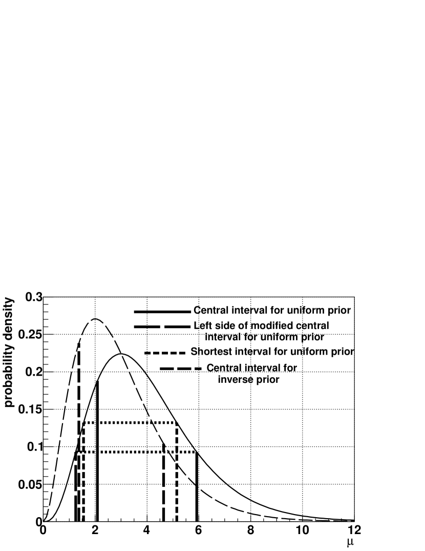
Figure 1: Probability densities for $\mu$ of the Poisson distribution (the one-channel problem without background), if 3 events are observed. The solid (dashed) smooth line depicts the probability density distribution for the uniform (inverse) prior. The intervals calculated with $\alpha=0.158655$ are shown by solid and dashed thick lines with different length of dashes. Dotted lines show horizontal levels.

If the area cut from each side of the distribution is denoted by $\alpha$ (and restricted by $\alpha<0.5$), the lower and upper boundaries $s_{\mathrm{L}}$ and $s_{\mathrm{U}}$ are defined by

$$\int_{s_{\mathrm{L}}}^{\infty}p(s|\vec{n})\,\mathrm{d}s=1-\alpha,\ \ \displaystyle\int_{0}^{s_{\mathrm{U}}}p(s|\vec{n})\,\mathrm{d}s=1-\alpha.$$ (12)

Cousins [1] showed that for the one-channel Poisson measurement with known nuisance parameters the use of the uniform prior for the main parameter results in an upper limit that covers the true value exactly with the stated probability and in a lower limit that covers with lower probability. Conversely, with the use of the inverse prior the lower limit covers correctly and the upper limit insufficiently. Another problem is that if the most probable $s$ is zero or close to zero, its value can be excluded from the credible interval, which raises doubts about the consistency of the whole approach.

For example, the confidence intervals calculated by different methods for a one-channel problem with known auxiliary parameters $a=1$ and $b=5$, $t_{a}=t_{b}=1$, for different observed $n$ are shown in Fig. 2.

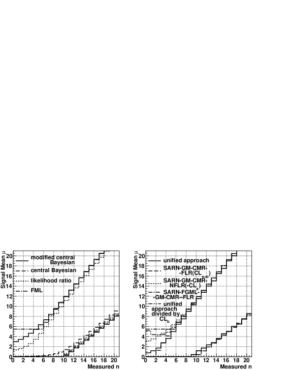
Figure 2: The confidence intervals for the one-channel problem with known auxiliary parameters $a=1$ and $b=5$, $t_{a}=t_{b}=1$, for different observed $n$ by different methods. The upper limit of the central Bayesian interval is not seen because it coincides by definition with the upper limit of the modified central Bayesian interval. The lower limit of the central Bayesian interval is the highest among the other lower limits. The upper limit for SARN–GM–CMR–FLR ($CL_{s+b}$) is very close to zero for $n$ equal to $0$ and $1$, but is not zero. The lower limit for SARN–GM–CMR–NFLR (LHC $CL_{s}$) coincides by definition with that of SARN–GM–CMR–FLR ($CL_{s+b}$) and both are lower than the lower limit for the unified approach. The lower limit of the unified approach coincides by definition with that of the unified approach divided by $CL_{b}$. The upper limit for the latter is defective because it increases for reducing $n\leq 3$. The lower limit of SARN–FGML–GM–CMR–FLR turns out to be numerically equal to that of SARN–GM–CMR–NFLR in this problem.

One can see that the lower limit of the Bayesian central credible interval does not include $s=0$ even at $n<5$, although it is very low.

The shortest interval includes the maximum due to the method of its construction, but does not provide good coverage, as was shown in [1] and obtained also for the examples considered herein.

One can also construct a level-based interval as it is done in the likelihood ratio method, that is using a level found with the Gaussian approximation. Writing the integral of the Gaussian in the form

$$F(z)=\frac{1}{\sqrt{2\pi}}\displaystyle\int_{-\infty}^{z}e^{-t^{2}/2}\,\mathrm{d}t$$ (13)

one obtains $z$ for given p-value, which is the same as $\alpha$ in our notations, by $z=F^{-1}(1-\alpha)$. If $\hat{s}$ is the most probable value that maximizes $p(s|\vec{n})$, see Eq. (10) or (11), the interval boundaries are set at the probability density smaller by the factor of $e^{-z^{2}/2}$. One has to find the lowest and the uppermost boundaries $s_{\mathrm{L}}$ and $s_{\mathrm{U}}$ such that $p(s_{\mathrm{L}}|\vec{n})=p(s_{\mathrm{U}}|\vec{n})=p(\hat{s}|\vec{n})e^{-z^{2}/2}$. If non-negative $s_{\mathrm{L}}$ does not exist, it is set to zero. These intervals appear to be close to the shortest intervals shown in Fig. 1 and have the same benefits and drawbacks.

The use of the right boundary of the central interval with the uniform prior and the left boundary of the central interval with the inverse prior (see Fig. 1) provides coverage, but does not always provide the inclusion of the most probable value. The left boundary can never be exactly zero.

But all mentioned problems are solved if one takes the right boundary from the central interval Eq. (12) computed with the uniform prior, and sets the left boundary at the same level of probability density as that for the right boundary, see Fig. 1. Graphically, one should draw a horizontal line from the upper edge of the right boundary to the left till its crossing with the distribution. If the non-negative $s_{\mathrm{L}}$ satisfying this condition does not exist, it is equated to zero. If the left boundary of the classical central interval is lower for any reason, it has to be used instead of this modified boundary. Calculations of the simple one-channel problem without background for various $n$ show that this modified boundary is always lower and usually almost equal to the lower boundary of the central interval for the inverse prior, which allows one to conclude that it should not undercover. Hence these “modified central intervals” cover by both ends for this simple problem.

In this method the probability of violating the lower limit can be smaller than $\alpha$. In the case of small signal it can even be zero.

3.7 The coverage and width of modified central intervals

If nuisance parameters are known, the coverage of the Bayesian modified central intervals is provided for all fixed divisions, see Fig. 3.

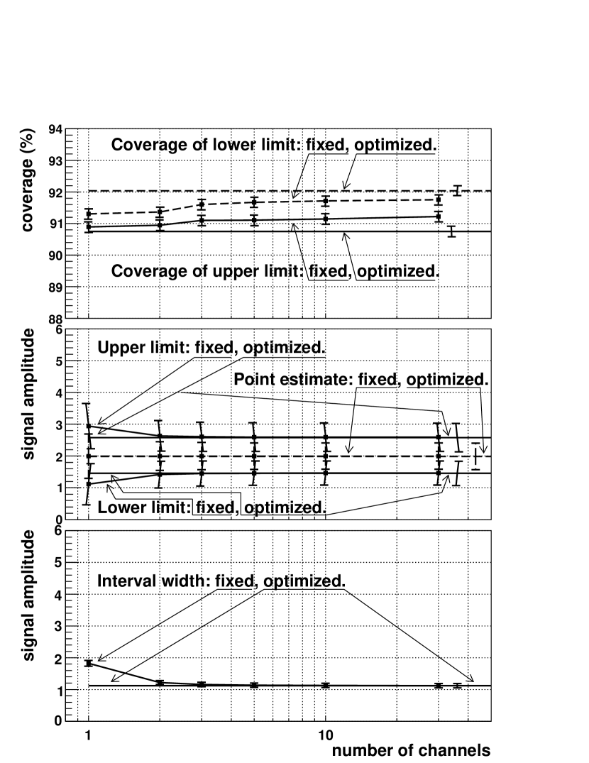
Figure 3: The Bayesian method, the modified central intervals for 90% ($\alpha=0.1$), no nuisance parameter uncertainties. The horizontal straight lines are results of optimization by interval widths. The optimization by separate interval boundaries results in coverage of about 83%.

In this figure and in the following ones the $x$-axis is identical in all three plots and represents the number of channels. The $y$-axes are different. In the top plot the $y$-axis shows the probability of coverage in percent. In the two lower plots $y$-axes are measured in the units of the total signal rate (or “signal amplitude”) $s$, but have different meanings. In the middle plot the $y$-axis means the position of the interval boundaries (i.e. the confidence limits) or of the point estimates. Since two different values are plotted in a single plot, the axis is labeled by the unit of their measurement “signal amplitude”. In the lower plot it means the interval widths and labeled similarly.

The points located at 1, 2, 3, 5, 10 and 30 channels and connected by lines display the results for fixed divisions. To show that the optimized-division results are not linked to a certain fixed number of channels, the optimized results are plotted as horizontal straight lines going beyond the used 30-channel limit with single error bars positioned somewhere at a larger number of channels (this position does not have any other meaning except showing that this is not the real number of channels). Recall that a different division can be chosen for each experiment, when the division is “optimized” using the information available in the particular experiment.

The points connected by the solid and dashed lines in the upper plot represent the coverage of the upper and lower interval boundary, respectively.

In the middle plot both the upper and lower limits are shown by the points connected by solid lines. The point estimates (the maxima of the Bayesian posterior) are the points connected by the dashed line. Obviously, the latter reside between the former.

The error bars in the uppermost coverage plots indicate the uncertainty of calculations for the standard 68% confidence level. These are frequentist uncertainties for the binomial distribution at the given number of experiments [34]. These uncertainties appear owing to the limited statistics of Monte Carlo simulations performed for this paper. In this particular plot they are very small due to very large simulated statistics. The Bayesian analysis without nuisance uncertainties is very quick.

The points and horizontal lines in the two lower plots show the arithmetic averages of the respective values over many experiments. All errors drawn in the two lower plots express the fluctuations of the respective values occurring experiment by experiment. To make the image more clear, the bars corresponding to upper limits are slightly inclined to the left, and the bars corresponding to lower limits to the right. The same inclination (not seen clearly in Fig. 3 because the bars are too short) is present also in the coverage plots. The errors in the two lower plots are calculated as the root-mean-square deviations and hence correspond to the standard 68% confidence level too.

Interestingly enough, the coverage for fixed numbers of channels presented in the uppermost plot, is almost constant and stays near 91% for all divisions for the studied example. But the interval widths and boundaries reach the plateau starting from 2 channels. For this case without nuisance uncertainties all the other reasonable methods behave similarly. According to similar calculations the lower boundary of the Bayesian central intervals (not modified) does not provide the stated coverage, as expected.

Thus, for the case with known nuisance parameters the modified Bayesian central intervals provide frequentist coverage.

The mean point estimates in the middle plot almost coincide with the true value of the parameter of interest, $s_{\mathrm{true}}=2$, both for fixed and for optimized divisions, so one cannot distinguish visually two dashed lines in this plot.

If the background uncertainties are switched on, the modified Bayesian method with safe priors behaves as shown in Fig. 4. The same case with hybrid priors gives almost an identical picture. In such figures the upper and lower limits form a valley with narrowing in the middle. In the middle plot one can also see additional dotted lines, which display the mean point estimates (maxima of the posteriors) calculated with the priors appropriate for the upper and lower limit. It is seen that they deviate from the optimal position simultaneously with the corresponding limits with the increase in the number of channels. Obviously this divergence is entirely due to the priors. Their arithmetic averages drawn by the dashed line for fixed divisions and by the straight dashed line for optimized divisions are very close to the true $s$.

Figure 4: The Bayesian method, the modified central intervals for 90% ($\alpha=0.1$), the uncertainty of the expected background, the known expected signal, safe nuisance priors. The horizontal lines are results of optimization by interval widths. Other details are described in Section 3.7 and in Fig. 3.

The same calculations with exchanged safe priors, where the uniform prior is used for the upper limit and the inverse prior for the lower one, give catastrophic results shown in Fig. 5. At more than 15 channels the lower limit becomes greater than the upper limit!

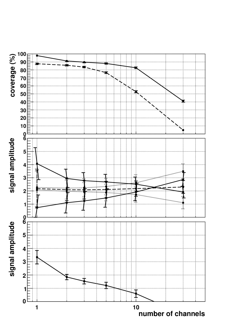
Figure 5: The Bayesian method, the modified central intervals for 90% ($\alpha=0.1$), the uncertainty of the expected background, the known expected signal, exchanged safe nuisance priors. Other details are described in Section 3.7 and in Fig. 3.

The priors $1/\sqrt{\mu}$ produce almost exact point estimates and not diverging limits for this example, but at the other parameters they lead to deviations anyway.

As shown in Fig. 4, the optimization of the division by the interval width provides almost perfect 90% coverage for the Bayesian case. Obviously, the algorithm usually takes one of the medium divisions, which provides the shortest interval for given main and auxiliary experiments.

Thus, for the case of unknown expected background the modified Bayesian central intervals with safe nuisance priors provide frequentist coverage, which is sometimes conservative. The same intervals with hybrid nuisance priors are almost identical.

When only the uncertainty of the expected signal is present, only the lower limit was found to cover the true parameter with no less than stated probability for all fixed divisions for this method, see Fig. 6.

Figure 6: The Bayesian method, the modified central intervals for 90% ($\alpha=0.1$), the uncertainty of the expected signal, the known expected background, safe nuisance priors. The horizontal lines are results of optimization by interval widths without zeros in the expected signal. Other details are described in Section 3.7 and in Fig. 3.

The coverage of the upper limit falls from 92% for 1 channel to 86% for 30 channels. This effect is even stronger with hybrid priors. The same effect appears in all other methods that use the safe or hybrid priors. The exchanged priors provide even worse coverage for the upper limit.

The reason for this pathology is simpler to illustrate for the Bayesian case. It has similar reasons for the other cases. The channels having the downward fluctuation of the expected signal and $n_{ai}=0$ do not influence the result because in such channels $a_{i}$ is distributed very close to zero due to the use of the inverse prior and $f_{i}=t_{a}a_{i}s+t_{b}b_{i}$ does not depend on $s$. Only the rest of the channels, where $n_{ai}$ could fluctuate upward, influence the result. Since $a_{i}$ seems to be greater for such channels than it is in the average, a smaller signal is enough to describe the observed result. Calculations indicate that not only zero $n_{ai}$ but also low non-zero values of $n_{ai}$ affect the result too. Apparently, the channels with downward fluctuations of $n_{ai}$ are more strongly masked by the background and participate less in the result, than the channels with larger $n_{ai}$.

Choosing the division with the least width without zeros in the distribution of the expected signal allows one to obtain the upper limit with coverage slightly smaller than requested, as indicated by the horizontal solid lines in the upper plots in Fig. 6. Some small lack of coverage is deemed to be tolerable.

It seems unlikely that one will ever have zero or close to zero content in a channel of the expected-signal distribution. This problem is more probable for the expected background.

The exchange of the priors affect less on the lower limit in the case of the uncertain expected signal, but it still affects strongly on the upper limit.

When both uncertainties of expected background and signal are switched on, the behavior of all characteristics for the test example studied is qualitatively the same as for the case only with the background uncertainty.

4 Frequentist Treatment of
Maximum Likelihood
Estimate

4.1 Introduction, the case without uncertainties.

Ciampolillo [23] and, independently, Mandelkern and Schultz [7] recently pointed out that the maximum likelihood estimate of the parameter of interest is a good test statistic for constructing frequentist confidence intervals for Poisson measurements with known expected signal and background. As they found, this test statistic allows one to avoid unphysical empty or nearly empty intervals in the case of downward background fluctuations, from which the frequentist analyses with other test statistics suffer. It can be added that obtaining limits for the parameter of interest by testing this very parameter is more straightforward, as well as convenient, than doing this by testing another variable, such as a likelihood ratio, whose behavior is difficult to predict in practical situations.

Here we call this method “FML”, which means “Frequency of Maximum Likelihood”.

The typical confidence belt for FML is shown in Fig. 7. This figure depicts the case of 5 channels with standard parameters for 10% one-sided confidence level with known expected signal and background. The notation $\hat{s}$ means the value of $s$ that maximizes $P(\vec{n}|s)$, which is here equal to $P(\vec{n}|t_{a}\vec{a}s+t_{b}\vec{b})=\prod_{i=1}^{k}\mathrm{Poisson}(n_{i},t_{a}a_{i}s+t_{b}b_{i})$. It is assumed that $\hat{s}$ is searched for in the non-negative interval $[0,\infty[$. For each assumed or possible $s$ we can simulate a set of pseudo-experiments and obtain the distribution of $\hat{s}$. These distributions are shown in this figure by the horizontal rows of boxes with variable size.

After choosing a specific value of $s$ for the current trial one generates a set of pseudo-experiments with it. This process will be called subgeneration, in order to distinguish it from the generation of “real” experiments. In this work the latter are simulated by the Monte Carlo method too, but this is done in the separate main program with the true parameters (which is not the case for subgeneration, see Section 2.2).

The probability density distribution of $\hat{s}$ at given $s$ in the “subgenerated” experiment is denoted by $p(\hat{s}_{\gamma}|s)$. The index $\gamma$ is included in order to indicate that the result is obtained by subgeneration. The integrals

$$\displaystyle\int_{\hat{s}_{\mathrm{right}}}^{\infty}p(\hat{s}_{\gamma}|s)\,\mathrm{d}\hat{s}_{\gamma}=\alpha$$ (14)

and

$$\displaystyle\int_{0}^{\hat{s}_{\mathrm{left}}}p(\hat{s}_{\gamma}|s)\,\mathrm{d}\hat{s}_{\gamma}=\alpha$$ (15)

allow us to plot the boundaries of the confidence region, which are depicted in Fig. 7 by thick inclined solid trajectories $[\mathrm{U}_{0},\mathrm{U}_{4}]$ and $[\mathrm{L}_{0},\mathrm{L}_{4}]$.

For the measurement C₂ the confidence interval is given by $[\mathrm{L}_{2},\mathrm{U}_{2}]$, which includes the true $s$ if it is depicted, for example, by $[\mathrm{A},\mathrm{B}]$. For the measurement C₃ the confidence interval $[\mathrm{L}_{3},\mathrm{U}_{3}]$ does not include this $s$. The proof of the one-sided coverage of the lower limit is based on the idea that the probability for $\mathrm{L}_{3}$ to be higher than $s$ is equal to the probability for $\mathrm{E}_{3}$ to be to the right of $\mathrm{F}$, and the latter is equal to $\alpha$ according to Eq. (14) or possibly smaller than $\alpha$ in the discrete case. The coverage of the upper limit is proved similarly by the points $\mathrm{U}_{1}$, $\mathrm{E}_{1}$ and $\mathrm{G}$.

Figure 7: Distribution of the observed most probable $s$ (denoted as $\hat{s}$) as a function of the true $s$ for 5 channels with known expected signal and background. See text for other notations.

These trajectories look like lines and this was assumed in the paragraph above, but in reality $\hat{s}$ can have discrete values only. The values of the limits in these points are only important. In the conditions of Fig. 7 these points are very close to each other and are merged in lines. Let us search the solution of Eq. (14) by replacing $\hat{s}_{\mathrm{right}}$ by $\hat{s}$ obtained for observed $\vec{n}$, which we denote here by $\hat{s}_{\mathrm{obs}}$. Then we have to fit $s$ to obtain the equality in this expression. Let us assume that the statistics of subgeneration is (nearly) infinite. Then the corresponding equation in the discrete form is

$$\sum_{\begin{subarray}{c}\vec{n}_{\gamma}:\\ \scriptsize{\makebox[25.6073pt][l]{$\hat{s}_{\gamma}(\vec{n}_{\gamma},\vec{a},\vec{b})\geq\hat{s}_{\mathrm{obs}}$}}\end{subarray}}P(\vec{n}_{\gamma}|s,\vec{a},\vec{b})=\alpha,$$ (16)

where $P(\vec{n}_{\gamma}|s,\vec{a},\vec{b})=\prod_{i=1}^{k}\mathrm{Poisson}(n_{\gamma i},t_{a}a_{i}s+t_{b}b_{i})$. It is meant here that only those $\vec{n}_{\gamma}$ are included for which the condition under the sign of sum is satisfied. If this sum is greater than $\alpha$ at $s=0$, zero $s$ is taken as the solution. This solution is the lower confidence limit $s_{\mathrm{L}}$. Note that this summing up should start from $\hat{s}_{\mathrm{obs}}$, not from the next allowed $\hat{s}_{\gamma}$ as it might seem at first glance. It is important because the value of this very sum calculated for $s=0$ can be used as the significance of signal$+$background hypothesis versus the simple background hypothesis. Obviously, the greater is $\hat{s}_{\mathrm{obs}}$, the more the event is signal-like. Significance is estimated as the probability for the test statistic to exceed the observed value or to coincide with it.

If we neglect discrete effects and some other mathematical details, which can make the coverage conservative, we can find out that the accurate coverage of intervals for any $\alpha$ is guaranteed by construction if and only if the subgenerated $\hat{s}_{\gamma}$ calculated at the true $s$ is distributed exactly as the experimental $\hat{s}$ after the imaginary repetitions of the experiment. If $\vec{a}$ and $\vec{b}$ are not known exactly, the coverage is not guaranteed by construction.

Since $\hat{s}$ is restricted to be non-negative, in the experiments where the formal $\hat{s}$ found in the interval $]-\infty,+\infty[$ is negative, $\hat{s}$ found in $[0,+\infty[$ is usually zero. This results in the appearance of a spike at zero in the distribution of $\hat{s}$, which is described by the $\delta$-function with a certain weight. This weight is negligible at high $s$. As $s$ decreases, this weight increases and at some point it becomes greater than $\alpha$. In Fig. 7 this is crossing of the upper limit $[\mathrm{U}_{0},\mathrm{U}_{4}]$ with the $y$-axis, that is the point $\mathrm{U}_{0}$. This spike should be excluded entirely from the integral in Eq. (15) and included in the confidence region. The sign “$=$” in Eq. (15) has to be replaced by “$\leq$”.

If we want to keep constant the area inside the two-sided interval, we have to shift the right boundary in order to cut off the right tail with the $2\alpha$ area instead of single $\alpha$. Thus, the full lower boundary will pass through the points $\mathrm{L}_{5},\mathrm{L}_{6},\mathrm{L}_{7},\mathrm{L}_{1},\mathrm{L}_{2},\mathrm{L}_{3},\mathrm{L}_{4}$. This very case was considered in Refs. [7, 23]. In this case the probability for the obtained lower limit to be higher than the true $s$ is unknown. It varies as a function of the true $s$ and can be either $\alpha$ or $2\alpha$, depending on the position of the point $\mathrm{U}_{0}$. If the latter is not determined and reported, it will also be unknown.

For comparison, boundaries of the shortest intervals and the low boundary of the modified central intervals in the Bayesian analysis cut the variable probability, but it can be easily calculated. Here the coverage cannot be directly calculated, and cannot be calculated at all, if one strictly follows the frequentist approach and does not consider the probability distribution of the true parameter of interest.

On the other hand, if the researcher does not shift the lower boundary when $s$ is below $\mathrm{U}_{0}$, the coverage by the lower limit will be constant, but the simultaneous “two-sided” coverage of the true $s$ by both limits will be either $1-\alpha$ or $1-2\alpha$. However, this two-sided coverage is less important in practice. There are exceptions, but usually this probability does not have any useful meaning. The violation of the lower and upper border usually leads to different physical conclusions and their separate confidence levels are the only values which are important. Therefore, the confidence belt restricted by $[\mathrm{U}_{0},\mathrm{U}_{4}]$ from above and $[\mathrm{L}_{0},\mathrm{L}_{4}]$ from below is tested in this research.

Calculations indicate that such a technique provides plots almost identical to the plots obtained by the modified central Bayesian intervals for the case of known nuisance parameters, see Fig. 3. The one-sided coverage of both upper and lower boundaries for fixed divisions, as well as for the divisions optimized by the interval width, stays near 90% in all cases. Differences in the lower two plots are negligible. Fig. 2 indicates that at the low observed signal the upper limit by FML can be higher than that for the Bayesian method. For the case with nuisance parameter uncertainties the method is split into many modifications, which will be described in the next section.

4.2 The case of unknown $\vec{a}$ and $\vec{b}$

If the values $\vec{a}$ and $\vec{b}$ are unknown, we have to use some approximations in the form of their assumed point values or probability densities. As in the Bayesian case, the naive ignoring of these uncertainties and the use of $\vec{n}_{a}$ instead of $\vec{a}$ and $\vec{n}_{b}$ instead of $\vec{b}$, as well as many other simple approaches, do not work well enough for FML in the example studied. More advanced assumptions are needed for the maximum likelihood finding with the data of the real experiment ($\hat{s}$), for the subgeneration of the experiment and for the maximum finding with the “subgenerated” data ($\hat{s}_{\gamma}$). We consider only the methods in which $\hat{s}$ and $\hat{s}_{\gamma}$ are found by an identical method. If $\hat{s}$ and $\hat{s}_{\gamma}$ are found differently, this subgeneration (with analysis) could never be realized as generation, that is we could not imagine such a sequence of experiments, for which our coverage and significance would be “true by construction”. When this feature is present, we call it the “modeling interpretation” or just the “interpretation”. Arguably, this modeling interpretation can be sufficient, if the frequentist coverage is unknown, but the model for nuisance parameters and the method of analysis are reasonable.

4.2.1 The SSP–FMML, SHP–FMML, and SEP–FMML methods

A simple method based on the assumption that the nuisance parameters are distributed randomly according to their posterior Bayesian probability density distributions (Eq. (9)) with safe (or hybrid) priors works well. In the following we assume that both $\vec{a}$ and $\vec{b}$ are unknown. The following expressions are simplified in an obvious way if one of them is known. The random values $a_{\gamma i}$ and $b_{\gamma i}$ are inserted in Eq. (1) or (2) and the result $f_{\gamma i}=t_{a}a_{\gamma i}s+t_{b}b_{\gamma i}$ is used to obtain $n_{\gamma i}$ of the subgenerated main experiment according to the Poisson distribution with mean $f_{\gamma i}$. One has to find the maximum $\hat{s}_{\mathrm{obs}}(\vec{n},\vec{n}_{a},\vec{n}_{b})$ of $p(s\,|\vec{n},\vec{n}_{a},\vec{n}_{b})$ and the maximum $\hat{s}_{\gamma}(\vec{n}_{\gamma},\vec{n}_{a},\vec{n}_{b})$ of $p(s\,|\vec{n}_{\gamma},\vec{n}_{a},\vec{n}_{b})$ for the observed and subgenerated data, respectively. In both cases the probability density distributions are given by Eq. (7) with substitution of Eqs. (8) and (9) or by Eq. (10) with substitution of Eq. (11) with the uniform prior for $s$ and with safe (or hybrid) priors for auxiliary $\vec{a}$ and $\vec{b}$. Because of the uniform prior for $s$, it is enough to find the maximum of Eq. (8) with substitution of Eq. (9) or the maximum of Eq. (11). Equation (16) can be rewritten as

$$\displaystyle\int\,p(\vec{a}_{\gamma}|\vec{n}_{a})\displaystyle\int\,p(\vec{b}_{\gamma}|\vec{n}_{b})\sum_{\begin{subarray}{c}n_{\gamma}:\\ \scriptsize{\makebox[25.6073pt][l]{$\hat{s}_{\gamma}(\vec{n}_{\gamma},\vec{n}_{a},\vec{n}_{b})\geq\hat{s}_{\mathrm{obs}}(\vec{n},\vec{n}_{a},\vec{n}_{b})$}}\end{subarray}}P(\vec{n}_{\gamma}|s,\vec{a}_{\gamma},\vec{b}_{\gamma})\,\mathrm{d}\vec{b}_{\gamma}\,\mathrm{d}\vec{a}_{\gamma}=\alpha\,.$$ (17)

Here $P(\vec{n}_{\gamma}|s,\vec{a}_{\gamma},\vec{b}_{\gamma})=\prod_{i=1}^{k}\mathrm{Poisson}(n_{\gamma i},t_{a}a_{\gamma i}s+t_{b}b_{\gamma i})$, which is equivalent to saying that $\vec{n}_{\gamma}$ is generated with current $s$, $\vec{a}_{\gamma}$ and $\vec{b}_{\gamma}$. The densities $p(\vec{a}_{\gamma}|\vec{n}_{a})$ and $p(\vec{b}_{\gamma}|\vec{n}_{b})$ are calculated by Eq. (9). Since Eq. (17) gives the lower limit, the uniform nuisance priors are used for calculations of $p(\vec{a}_{\gamma}|\vec{n}_{a})$, $p(\vec{b}_{\gamma}|\vec{n}_{b})$, $\hat{s}_{\gamma}(\vec{n}_{\gamma},\vec{n}_{a},\vec{n}_{b})$ and $\hat{s}_{\mathrm{obs}}(\vec{n},\vec{n}_{a},\vec{n}_{b})$. For the upper limit the inverse nuisance priors should be used (the hybrid median prior is allowed too). Some mathematical and numerical subtleties can be present in Eq. (17) and in other similar equations for different methods discussed here, because of the limited statistics and limited number of trials, as well as complex features of the methods. In particular, the least $s$ that satisfies the equation, should always be searched for. An analogous reversed approach is used for the upper limits.

Obviously, in the case of zero $s$ the expression at the left-hand side of Eq. (17) can be used as an estimate of $p$-value similarly to Eq. (16).

These variants of FML can be briefly denoted by FMML, “Frequency of Marginalized Maximum Likelihood”, or more explicitly by SSP–FMML or SHP–FMML, where the prefixes mean the Subgeneration with Safe Priors or Hybrid Priors, respectively. Other priors do not work satisfactorily. Note that the safe (or hybrid) priors are used not only for subgeneration, but for marginalization too, that is for the calculation of $\hat{s}_{\gamma}(\vec{n}_{\gamma},\vec{n}_{a},\vec{n}_{b})$ and $\hat{s}_{\mathrm{obs}}(\vec{n},\vec{n}_{a},\vec{n}_{b})$. It is implied unless otherwise specified.

According to Ref. [15], the $p$-value obtained by Eq. (17) at $s=0$ belongs to the category of “prior predictive $p$-values”. This notation can be confusing because $p(\vec{a}_{\gamma}|\vec{n}_{a})$ and $p(\vec{b}_{\gamma}|\vec{n}_{b})$ are posteriors for $\vec{n}_{a}$ and $\vec{n}_{b}$. But the “posterior predictive $p$-values” assume that the posteriors should also depend on $n$, which is not the case here.

These methods ensure the coverage by construction provided that the assumption at the beginning of this section is true. This is easily realized in practice if one does not repeat the auxiliary experiments and treats the sequence of the main experiments with the initially observed $\vec{n}_{a}$ and $\vec{n}_{b}$. So the reasonable modeling interpretation exists for this method. Similarly, this method provides an interesting feature of self-consistency of the $p$-value. For given $\vec{n}_{a}$ and $\vec{n}_{b}$ the probabilities of $\vec{n}_{\gamma}$ used for calculation of $p$-value by the left-hand side of Eq. (17) do not depend on $\vec{n}$. Let us denote $p$-values calculated for any $\vec{n}_{1}$ and $\vec{n}_{2}$ and for the same $\vec{n}_{a}$ and $\vec{n}_{b}$ by $\rho(\vec{n}_{1},\vec{n}_{a},\vec{n}_{b})$ and $\rho(\vec{n}_{2},\vec{n}_{a},\vec{n}_{b})$, respectively. Then for any such $\vec{n}_{1}$ and $\vec{n}_{2}$, if $\hat{s}_{\mathrm{obs}}(\vec{n}_{1},\vec{n}_{a},\vec{n}_{b})>\hat{s}_{\mathrm{obs}}(\vec{n}_{2},\vec{n}_{a},\vec{n}_{b})$, all $\vec{n}_{\gamma}$ that are taken into account for $\rho(\vec{n}_{1},\vec{n}_{a},\vec{n}_{b})$ should also be taken into account for $\rho(\vec{n}_{2},\vec{n}_{a},\vec{n}_{b})$, but at least one $\vec{n}_{\gamma}=\vec{n}_{2}$ that is taken into account for $\rho(\vec{n}_{2},\vec{n}_{a},\vec{n}_{b})$ should not be taken into account for $\rho(\vec{n}_{1},\vec{n}_{a},\vec{n}_{b})$. Therefore $\rho(\vec{n}_{2},\vec{n}_{a},\vec{n}_{b})>\rho(\vec{n}_{1},\vec{n}_{a},\vec{n}_{b})$. This means that if one uses the $p$-value $\rho$ as the test statistic for calculation of another $p$-value, one obtains an alternative $p$-value (see Section 1.4), which should be equal to the regular $p$-value. The both $p$-values are also uniformly (taking into account discreteness) distributed in $[0,1]$ for fixed $\vec{n}_{a}$ and $\vec{n}_{b}$. This equality and uniformity is not guaranteed for many other methods, for which the probabilities of $\vec{n}_{\gamma}$ used for calculation of $p$-values are different for different $\vec{n}$.

To test different priors SSP–FMML was also run with exchanged priors, so that the uniform prior was used for the upper limit and the inverse prior was used for the lower limit. This method is denoted here by prefix SEP (Subgeneration with Exchanged Priors) with full notation SEP–FMML. The exchanged priors are used for marginalization too.

Figure 8: The SSP–FMML method, confidence intervals for 90% one-sided confidence ($\alpha=0.1$), the uncertainty of the expected background, the known expected signal. The horizontal lines are results of optimization by the widths of modified central Bayesian intervals. Other details are described in Sections 4.2.1, 3.7, and in Fig. 3.

The calculations have shown that the SSP–FMML and SHP–FMML methods have characteristics that are very similar to those of the Bayesian methods with respective priors and with modified central intervals, described earlier. For example, the case with uncertainty of the expected background is shown in Fig. 8. The upper limit for SHP–FMML is lower apporximately by 0.1. The coverage of SHP–FMML is similar. The optimization of the division with the Bayesian modified central intervals provides reasonably good coverage of the optimized limits obtained by both methods. The optimization with the intervals obtained by these methods themselves provides slightly worse coverage of the upper limit. Each of these methods, as well as the Bayesian one, produces two point estimates, which have to be averaged.

The analysis by SEP–FMML behaves similarly to the Bayesian analysis with modified central intervals and with exchanged priors, which is described in Section 3.7. This method can yield completely wrong results.

Since the lower limit and the $p$-value are calculated effectively by the same equation (17), the lower limits by SSP–FMML are reliable, its modeling interpretation is convincing and the significance is self-consistent for fixed $\vec{n}_{a}$ and $\vec{n}_{b}$, one might expect that the significance by this method is reliable too. It is however difficult to find any exclusive numerical feature of significance by SSP–FMML besides self-consistency, which is inherent to many other methods as well. One can compare the significance calculated by Eq. (17) with the exact significance $z_{\mathrm{ef}}$, whose $p$-value is defined by

$$\rho_{\mathrm{ef}}(\vec{n},\vec{n}_{a},\vec{n}_{b})=\sum_{\begin{subarray}{c}\vec{n}_{\gamma p}:\\ \scriptsize{\makebox[42.67912pt][l]{$\hat{s}_{\gamma}(\vec{n}_{\gamma},\vec{n}_{a},\vec{n}_{b})\geq\hat{s}_{\mathrm{obs}}(\vec{n},\vec{n}_{a},\vec{n}_{b})$}}\end{subarray}}P(\vec{n}_{\gamma}|s=0,\vec{a},\vec{b}),$$ (18)

where the subscript “e” means “exact”, “f” means “fixed”, that is the fixed nuisance parameter measurements $\vec{n}_{a}$ and $\vec{n}_{b}$, and for the fitting of $\hat{s}$-values one should take into account that the nuisance parameters are unknown. The corresponding significance will be called $z_{\mathrm{ef}}$. If only the expected signal is unknown, the approximate significance (that is the estimate of significance by SSP–FMML, whose $p$-value is calculated according to Eq. (17)) turns out to be identical to $z_{\mathrm{ef}}$, but this holds also for SEP–FMML, which gives slightly greater significance for many-channel problems. This holds also for any other methods with prefixes SSP or SEP, described later. Note also that the exact $p$-value can be defined with random subgenerated nuisance parameter measurements and obtained from Eq. (18) by replacement of $\hat{s}_{\gamma}(\vec{n}_{\gamma},\vec{n}_{a},\vec{n}_{b})$ by $\hat{s}_{\gamma}(\vec{n}_{\gamma},\vec{n}_{a\gamma},\vec{n}_{b\gamma})$. Let us denote this by the subscript “r”, random. Comparing the approximate significance with $z_{\mathrm{ef}}$ or $z_{\mathrm{er}}$ we simply assume different frequentist interpretations of our approximate significance. When only the expected background is unknown, the approximate significance by SSP–FMML is usually less than $z_{\mathrm{er}}$ (which is acceptable), but not always. It is not usually less than $z_{\mathrm{ef}}$. Moreover, both exact significances, minimized with respect to $\vec{a}$ and $\vec{b}$, are usually zero, except the case of $z_{\mathrm{ef}}$ and $\vec{a}$, see above. However, there is another test statistic based on likelihood ratios with marginalization, described in Section 6.2.2, and providing nontrivial minima of $z_{\mathrm{er}}$. Calculations indicate that the approximate significance by SSP–FMML is usually less than this minimal significance, but there are better approximate methods. So the significance by this method can be used, but there are more reliable methods. The confidence intervals by this method are very reliable.

4.2.2 The SSP–FGML, SHP–FGML, and SEP–FGML methods

Another approach alternative to (SSP–)FMML consists in finding the global maximum of the common likelihood given by Eq. (4) and expressed by $P(\vec{n},\vec{n}_{a},\vec{n}_{b}|\hat{s}_{\mathrm{obs}},\hat{\vec{a}}_{\mathrm{obs}},\hat{\vec{b}}_{\mathrm{obs}})$ for the case of the observed data, instead of the maximum of the Bayesian posterior as required for FMML. The subgeneration can be performed exactly as for SSP–FMML. For the analysis of the subgenerated experiments it needs to find the global maximum $P(\vec{n}_{\gamma},\vec{n}_{a},\vec{n}_{b}|\hat{s}_{\gamma},\hat{\vec{a}}_{\gamma},\hat{\vec{b}}_{\gamma})$ with respect to $\hat{s}_{\gamma}$, $\hat{\vec{a}}_{\gamma}$, and $\hat{\vec{b}}_{\gamma}$. Equation (17) is not changed, except that the values $\hat{s}_{\gamma}(\vec{n}_{\gamma},\vec{n}_{a},\vec{n}_{b})$ and $\hat{s}_{\mathrm{obs}}(\vec{n},\vec{n}_{a},\vec{n}_{b})$ have a different sense, which is described above. The modeling interpretation of this method is similar to that of SSP–FMML. The $p$-values are self-consistent.

In this method the Bayesian priors are used only for subgeneration. For maximization the priors are not used. Hence the observed $\hat{s}_{\mathrm{obs}}(\vec{n},\vec{n}_{a},\vec{n}_{b})$ is single and should not be averaged to obtain the final point estimate as necessary for the Bayesian and FMML cases. It has some systematic shift, but the latter is not large.

This variant of FML can be called SSP–FGML or SHP–FGML, Subgeneration with Safe (or Hybrid, respectively) Priors, Frequency of Global Maximum Likelihood. As with SEP–FMML, one can consider FGML with Subgeneration with Exchanged Priors, SEP–FGML, but it does not provide satisfactory results.

Calculations indicate that all performance characteristics of SSP–FMML and SSP–FGML (or SHP–FMML and SHP–FGML, respectively) are almost the same with four exceptions which are worth mentioning. First, the upper limit for one channel has almost 100% coverage. Second, the upper and the lower limit diverge less at 30 channels for FGML than they do for FMML in Fig. 8. Instead of the average interval width equal to approximately 3.9 units for SSP–FMML (about 3.8 for SHP–FMML) the SSP–FGML method gives about 3.5 units (about 3.3 for SHP–FGML). Third, the coverage of the upper optimized limit ($90.0\pm 0.6\%$) is slightly higher than that for FMML ($87.9\pm 0.6\%$, see Fig. 8). Fourth, the calculations by FGML are faster with the existing program than that by FMML. However, FGML finds the most probable values of the main parameter taking into account the most probable nuisance parameters and ignoring the other possible values of them, whereas FMML takes into account all of them. The latter is more appealing conceptually and also technically, if the nuisance parameter is predicted from general theoretical considerations as an interval of allowed values, with unknown and hence equal probabilities inside this range. Another example of failure to determine $\hat{s}$ by FGML is the one-channel problem with expected-signal uncertainty at $n_{a}=0$ and $b\geq n$, where the likelihood does not depend on $s$ (in this work it is assumed that $\hat{s}=0$ for this case). Advantages of the “integrated likelihood” are also discussed in Ref. [35]. Faster calculations by global maximization by our software and taking into account all possible values of nuisance parameters with possibility to apply plain distributions in the case of marginalization are inherent to all the other discussed methods that use these approaches (we will not repeat this each time).

4.2.3 The SSPRN–FMML and SSPRN–FGML
methods

In both SSP–FMML and SSP–FGML the auxiliary measurements are not generated at the subgeneration stage. The question is whether one could obtain a method with better characteristics which uses the “subgenerated” auxiliary measurements. First of all, we can simply add the generation of the auxiliary measurements at the subgeneration stage into SSP–FMML and SSP–FGML and keep everything else the same. Then, Equation (17) is converted into

$$\displaystyle\int\,p(\vec{a}_{\gamma}|\vec{n}_{a})\displaystyle\int\,p(\vec{b}_{\gamma}|\vec{n}_{b}) \times$$

$$\sum_{\begin{subarray}{c}\vec{n}_{\gamma},\vec{n}_{a\gamma},\vec{n}_{b\gamma}:\\ \scriptsize{\makebox[42.67912pt][l]{$\hat{s}_{\gamma}(\vec{n}_{\gamma},\vec{n}_{a\gamma},\vec{n}_{b\gamma})\geq\hat{s}_{\mathrm{obs}}(\vec{n},\vec{n}_{a},\vec{n}_{b})$}}\end{subarray}}P( \vec{n}_{\gamma},\vec{n}_{a\gamma},\vec{n}_{b\gamma}|s,\vec{a}_{\gamma},\vec{b}_{\gamma})\,\mathrm{d}\vec{b}_{\gamma}\,\mathrm{d}\vec{a}_{\gamma}=\alpha\,.$$ (19)

Here $n_{a\gamma i}$ and $n_{b\gamma i}$ are generated according to the Poisson distributions with parameters $a_{\gamma i}$ and $b_{\gamma i}$, respectively. The value $\hat{s}_{\gamma}(\vec{n}_{\gamma},\vec{n}_{a\gamma},\vec{n}_{b\gamma})$ is calculated as usually for SSP–FMML or SSP–FGML. Inserting the suffix “RN” (Random Nuisance) into the old notations we obtain the notations SSPRN–FMML and SSPRN–FGML. In the case of SSPRN–FMML the use of Eq. (7) with substitution of Eqs. (8) and (9) for the fitting of $\hat{s}_{\gamma}(\vec{n}_{\gamma},\vec{n}_{a\gamma},\vec{n}_{b\gamma})$ implies that $\vec{a}_{\gamma}$ and $\vec{b}_{\gamma}$ are distributed according to $\vec{n}_{a\gamma}$ and $\vec{n}_{b\gamma}$, while they are really distributed according to $\vec{n}_{a}$ and $\vec{n}_{b}$ during the subgeneration.

In general, non-“RN” methods effectively (here the term “effectively” means that we ignore for the moment technical details like the type of the test statistic and many dimensions) compare $\vec{n}$ with $\vec{n}_{\gamma}$, but the “RN” methods compare some effective generalized relation of $\vec{n}$ and $\vec{n}_{b}$ together with $\vec{n}_{a}$ with a relation of $\vec{n}_{\gamma}$ and $\vec{n}_{b\gamma}$ together with $\vec{n}_{a\gamma}$. This can lead to strange situations when an experiment with $t_{b}\vec{n}_{b\gamma}$ effectively greater than $\vec{n}$ is not included in the $p$-value, if $\vec{n}_{\gamma}$ is yet greater. When $\vec{b}$ is known, the non-“RN” methods give the “exact” $p$-values in the sense that this or greater test statistic should be observed with exactly this probability independently of the unknown $\vec{a}$ after many repetitions of this experiment (see Section 4.2.1), but these $p$-values are different for different methods in the general case. It is easier to speed up the calculations by memorizing and recovering $\hat{s}_{\gamma}$ from some tables for non-“RN” methods, than for “RN” methods because of greater dimensionality of these tables in the last case.

Both SSPRN–FMML and SSPRN–FGML do not provide a realistic modeling interpretation of intervals and the corresponding modeled coverage by construction. The model from SSP–FMML does not work here because after the repetition of auxiliary experiments one would restore varying distributions of $\vec{a}_{\gamma}$ and $\vec{b}_{\gamma}$ and varying confidence regions. This is not a problem for the calculation of the $p$-value, which is given by the left-hand side of Eq. (19) at $s=0$. As with the FMML and FGML methods without the suffix “RN”, the $p$-value has to be reproduced in a long range of main and auxiliary experiments provided that $\vec{a}$ and $\vec{b}$ are distributed according to Eq. (9) calculated with the initially measured $\vec{n}_{a}$ and $\vec{n}_{b}$. However, the self-consistency of $p$-values is not guaranteed. For any two measurements denoted by subscripts “1” and “2”, if $\hat{s}_{\mathrm{obs}}(\vec{n}_{1},\vec{n}_{a1},\vec{n}_{b1})>\hat{s}_{\mathrm{obs}}(\vec{n}_{2},\vec{n}_{a2},\vec{n}_{b2})$, the value $\rho(\vec{n}_{2},\vec{n}_{a2},\vec{n}_{b2})$ should not necessarily be greater than $\rho(\vec{n}_{1},\vec{n}_{a1},\vec{n}_{b1})$. For example, if $n=67$, $t_{a}=1$, $a=1$, $t_{b}=2$, and $n_{b}=15$ (an example from table 1 of Ref. [14], discussed also in Section 7 herein), then $\hat{s}_{\mathrm{obs}}=36.4179$ and $\rho=0.000105$. If $n=65$ and $n_{b}=14$ with the same other parameters, then $\hat{s}_{\mathrm{obs}}=36.3893$ and $\rho=0.000075$. Therefore the self-consistency cannot be proved.

Numerical tests show that both SSPRN–FMML (see Fig. 9)

Figure 9: The SSPRN–FMML method, confidence intervals for 90% one-sided confidence ($\alpha=0.1$), the uncertainty of the expected background, the known expected signal. The horizontal lines are results of optimization by the widths of modified central Bayesian intervals. Other details are described in Sections 4.2.3, 3.7, and in Fig. 3.

and SSPRN–FGML behave similarly and do not provide frequentist coverage for the lower limit. Interestingly, the coverage is minimal for intermediate numbers of channels, 2–5 channels. When only the uncertainty of the expected signal is present, both methods behave similarly to the Bayesian approach, including the loss of the coverage of the upper limit for a large number of channels owing to zeros in the expected signal distributions. The significance calculated by them is usually greater and less reliable than that for SSP–FMML and SSP–FGML for unknown expected background and slightly less at unknown expected signal. If the priors are exchanged (these methods can be denoted by SEPRN–FMML and SEPRN–FGML) at unknown background, the coverage of the lower limits gets even worse, while the upper limits are not strongly changed. None of these methods can be recommended.

4.2.4 The SMRN–FGML and SARN–FGML methods

In the SMRN–FGML method the subgereration is done with the most probable nuisance parameters $\hat{\vec{a}}_{\mathrm{obs}}$ and $\hat{\vec{b}}_{\mathrm{obs}}$, which are determined by the global maximization of $P(\vec{n},\vec{n}_{a},\vec{n}_{b}|\hat{s}_{\mathrm{obs}},\hat{\vec{a}}_{\mathrm{obs}},\hat{\vec{b}}_{\mathrm{obs}})$. The prefix SMRN means the Subgeneration with the Most probable observed nuisance parameters and Random Nuisance parameter measurements. The global maximization is proposed in Ref. [23] (p. 1421) and more recently in Ref. [36]. In the SARN–FGML method the subgeneration is done with $\hat{\hat{\vec{a}}}_{\mathrm{obs}}$ and $\hat{\hat{\vec{b}}}_{\mathrm{obs}}$ that maximize $P(\vec{n},\vec{n}_{a},\vec{n}_{b}|s,\hat{\hat{\vec{a}}}_{\mathrm{obs}},\hat{\hat{\vec{b}}}_{\mathrm{obs}})$ for each given $s$. This idea is borrowed from the LHC-style $CL_{s}$ method, which is described in Section 6. On the other hand, this method can be considered as a modification of SMRN–FGML. The values $\hat{\hat{\vec{a}}}_{\mathrm{obs}}$ and $\hat{\hat{\vec{b}}}_{\mathrm{obs}}$ can be seen as adjusted for given $s$, which changes the abbreviation from SMRN to SARN: Subgeneration with Adjusted nuisance parameters and Random Nuisance parameter measurements.

The value $\hat{s}_{\mathrm{obs}}$ has to be used as the observed test statistic value. The ordinary FGML is applied to the subgenerated data. For the subgenerated experiments it needs to find the global maximum of $P(\vec{n}_{\gamma},\vec{n}_{a\gamma},\vec{n}_{b\gamma}|\hat{s}_{\gamma},\hat{\vec{a}}_{\gamma},\hat{\vec{b}}_{\gamma})$ with respect to $\hat{s}_{\gamma}$, $\hat{\vec{a}}_{\gamma}$, $\hat{\vec{b}}_{\gamma}$. The result $\hat{s}_{\gamma}$ is compared with $\hat{s}_{\mathrm{obs}}$. Equation (16) can be rewritten by

$$\sum_{\begin{subarray}{c}n_{\gamma},\vec{n}_{a\gamma},\vec{n}_{b\gamma}:\\ \scriptsize{\makebox[42.67912pt][l]{$\hat{s}_{\gamma}(\vec{n}_{\gamma},\vec{n}_{a\gamma},\vec{n}_{b\gamma})\geq\hat{s}_{\mathrm{obs}}(\vec{n},\vec{n}_{a},\vec{n}_{b})$}}\end{subarray}} P(\vec{n}_{\gamma},\vec{n}_{a\gamma},\vec{n}_{b\gamma}|s,\hat{\vec{a}}_{\mathrm{obs}},\hat{\vec{b}}_{\mathrm{obs}})=\alpha.$$ (20)

for SMRN–FGML and the same with replacement of $\hat{\vec{a}}_{\mathrm{obs}}$ and $\hat{\vec{b}}_{\mathrm{obs}}$ by $\hat{\hat{\vec{a}}}_{\mathrm{obs}}$ and $\hat{\hat{\vec{b}}}_{\mathrm{obs}}$, respectively, for SARN–FGML.

These methods do not have a reasonable interpretation of intervals. Indeed, if the main experiment is repeated, $\hat{\vec{a}}_{\mathrm{obs}}$ and $\hat{\vec{b}}_{\mathrm{obs}}$ for SMRN and $\hat{\hat{\vec{a}}}_{\mathrm{obs}}$ and $\hat{\hat{\vec{b}}}_{\mathrm{obs}}$ for SARN, which are used for subgeneration after each repetition, would be different each next time whether one repeats the auxiliary experiments or not, because they depend on $\vec{n}$. Even if the true $\vec{a}$ and $\vec{b}$ coincide with initially observed $\hat{\vec{a}}_{\mathrm{obs}}$ and $\hat{\vec{b}}_{\mathrm{obs}}$, the confidence belt would be different at each next repetition and the procedure used for the initial subgeneration could not be reproduced. The self-consistency of $p$-values is not guaranteed.

Figure 10: The SMRN–FGML method, confidence intervals for 90% one-sided confidence ($\alpha=0.1$), the uncertainty of the expected background, the known expected signal. The horizontal lines are results of optimization by the widths of modified central Bayesian intervals. Other details are described in Sections 4.2.4, 3.7, and in Fig. 3.

Figure 11: The SARN–FGML method, confidence intervals for 90% one-sided confidence ($\alpha=0.1$), the uncertainty of the expected background, the known expected signal. The horizontal lines are results of optimization by the widths of modified central Bayesian intervals. Other details are described in Sections 4.2.4, 3.7, and in Fig. 3.

According to calculations the frequentist coverage is not provided for the lower limit, see Figs. 10 and 11. The “standard” optimization of divisions (see Section 2.3) shown in these figures results in undecoverage of the lower limit for SMRN–FGML and moderate undecoverage of both limits for SARN–FGML. If the optimization is necessary and the coverage of the upper limit is important, one can choose to use SMRN–FGML for the upper limit and SARN–FGML for the lower one. A good optimized coverage of all these methods is obtained by the rejection of divisions with zeros in the expected-background distribution and choosing the most detailed division without zeros. But this optimization cannot be recommended because of its assumed poor performance in the presence of the truly zero channels in the expected background distribution (see Section 2.3) and because of the possibility of splitting into too many channels at large statistics. When only the uncertainty of the expected signal is present, the coverage of the upper limit by both methods is not reduced with the increase in the number of channels, but the optimized coverage is lower than necessary, about 86–88%.

The interpretation of the $p$-value is based on single and arguable values of $\vec{a}$ and $\vec{b}$ without considering alternatives, which can be unconvincing. The calculations show that significance is usually much greater than that for SSP–FMML and SSP–FGML for the case of uncertain background. Since the exact significances for SARN–FGML are the same as for SSP–FGML, the former should be, as a rule, less reliable.

5 Likelihood Ratio

As mentioned earlier, the probability density, given, for instance, by Eq. (4), can be considered as the likelihood of the parameters. We will not use here an additional notation for it (usually $L$). The likelihood ratio is denoted in some references by $\lambda$ and defined by

$$\lambda(s)=\frac{{P(\vec{n},\vec{n}_{a},\vec{n}_{b}|s,\hat{\hat{\vec{a}}},\hat{\hat{\vec{b}}})}}{P(\vec{n},\vec{n}_{a},\vec{n}_{b}|\hat{s},\hat{\vec{a}},\hat{\vec{b}})}\,.$$ (21)

Here the denominator is maximized with respect to all parameters, and the nominator is maximized only with respect to the nuisance parameters for the specified $s$. Here, as well as everywhere in this paper, all parameters are limited to their physical values, so they cannot be smaller than zero. In principle, this method can be applied also without this restriction, as in Refs. [10, 12], but here this option is not considered as having unclear physical sense.

Given $\alpha$ one should obtain $z$ as described after Eq. (13). Then the lowest $s_{\mathrm{L}}$ and the uppermost $s_{\mathrm{U}}$ that satisfy $\lambda(s_{\mathrm{L}}))=\lambda(s_{\mathrm{U}}))=e^{-z^{2}/2}$ are taken as limits. Alternatively, one can obtain the same limits from the fractile of the $\chi^{2}$-distribution with one degree of freedom, as recommended in Ref. [12]. Given $2\alpha$ one obtains $z^{2}$ and proceeds in the same way. If non-negative $s_{\mathrm{L}}$ does not exist, it is equated to zero.

Attractive features of this method are the absence of priors, simplicity and applicability for more generic problems, as well as its past success [22]. Its intervals should asymptotically converge to frequentist intervals for large statistics (see Ref. [22] and references in Ref. [1]), and they do not have meaning for non-Gaussian cases with small statistics.

The tests with the example studied here show that the coverage is slightly unstable and sometimes slightly insufficient, see Fig. 12. Optimization makes it worse. The “confidence” interval is shorter than that for the Bayesian method, SSP–FMML, and SSP–FGML, but it remains of the same order of magnitude, see Fig. 2. So this method can be used for fast estimates of intervals, but these intervals may be inaccurate and usually too short. Obviously, just like the Bayesian method, it cannot provide significance in a direct way, but an asymptotic approximation to $CL_{s}$ methods described later is closely related to it.

Figure 12: The likelihood ratio method, intervals for 90% one-sided “confidence” ($\alpha=0.1$), the uncertainty of the expected background, the known expected signal. The horizontal lines depict optimization by the width of these intervals. Other details are described in Sections 5, 3.7, and in Fig. 3.

6 Frequentist treatment of the likelihood ratio

6.1 Introduction, the case without uncertainties

Following notations of Read [9] we now denote the likelihood ratio by $Q$ and write

$$Q=\frac{P(\vec{n}|s)}{P(\vec{n}|s_{\mathrm{ref}})}\,.$$ (22)

For the present we will ignore the issues of nuisance parameters. The parameter $s_{\mathrm{ref}}$ is some reference value of $s$. According to the approach from Ref. [9] $s_{\mathrm{ref}}=0$. Here this approach will be called the “Background-Related” method and denoted by the abbreviation BR. This approach can be used for estimation of significance at known or assumed $s$ or for estimation of the upper limit of $s$ for predefined $\alpha$. According to a newer method, formulated in CERN for standard model Higgs boson search at the LHC [26, 27], $s_{\mathrm{ref}}$ maximizes $P(\vec{n}|s_{\mathrm{ref}})$, but it is constrained by $s_{\mathrm{ref}}\leq s$. We interpret this constraint in such a way that $s_{\mathrm{ref}}$ is initially found in the $[0,\infty[$ interval and, if it is greater than $s$, it is equated to $s$. This can be used for the upper limit. By analogy for the lower limit $s_{\mathrm{ref}}$ can be chosen such that it maximizes $P(\vec{n}|s_{\mathrm{ref}})$ and is constrained by $s_{\mathrm{ref}}\geq s$. The constraint allows us to set limits that exclude the fixed and usually equal portion of more signal-like events by the lower limit and the same portion of less signal-like events by the upper limit. This method will be denoted here by the suffix CMR, which means the “Constrained-Maximum-Related” method. $s_{\mathrm{ref}}$ can also be found in the $[0,\infty[$ interval without the additional constraints. In this case we mix the experiments that are outside both limits. One limit can exclude more experiments than another. This method is known as “the unified approach” [6]. We will denote it here by the suffix UMR, which means the “Unconstrained(or Unified)-Maximum-Related” method.

These methods can also be used for estimation of significance, if calculated with $s=0$. In this case the constraint duplicates the constraint assumed in the calculation of the global maximum $\hat{s}\geq 0$, so $s_{\mathrm{ref}}$ is simply equal to $\hat{s}$ and there is no difference between the CMR and UMR methods. The first character can be omitted in this case.

For instance, for the background-related method in the fully binned Poisson case the value of $Q$ is expressed [9] by

$$Q=\frac{\prod_{i=1}^{k}\frac{e^{-(t_{a}a_{i}s+t_{b}b_{i})}(t_{a}a_{i}s+t_{b}b_{i})^{n_{i}}}{n_{i}!}}{\prod_{i=1}^{k}\frac{e^{-{t_{b}b_{i}}}(t_{b}b_{i})^{n_{i}}}{n_{i}!}}=$$

$$=e^{-\sum_{i=1}^{k}t_{a}a_{i}s}\prod_{i=1}^{k}(1 +\frac{t_{a}a_{i}s}{t_{b}b_{i}})\,.$$ (23)

The work [9] also claims that “the confidence in the signal$+$background hypothesis is given by the probability that the test statistic is less than or equal to the value observed in the experiment, $Q_{obs}$:

$$CL_{s+b}=P_{s+b}(Q\leq Q_{obs})",$$ (24)

provided that $\vec{n}$ which is used for calculating $Q$ (during subgeneration, according to our terminology) is distributed according to the signal$+$background hypothesis, which is indicated by the subscript $s+b$. “Small values of $CL_{s+b}$ indicate poor compatibility with the signal+background hypothesis and favor the background hypothesis” [9]. According to the earlier work of Junk [24] $CL_{s+b}$ is “the confidence level for excluding the possibility of simultaneous presence of new particle production and background (the $s+b$ hypothesis)”. So this is the usual exclusion of the impossible, expressed, for instance, by Eq. (15) for the case of FML and used for setting the upper frequentist limit:

$$CL_{s+b}=P_{s+b}(Q\leq Q_{obs})=\sum_{\begin{subarray}{c}\vec{n}_{\gamma}:\\ \scriptsize{\makebox[28.45274pt][l]{$Q(\vec{n}_{\gamma},\vec{a},\vec{b},s)\leq Q(\vec{n},\vec{a},\vec{b},s)$ }}\end{subarray}}P(\vec{n}_{\gamma}|s,\vec{a},\vec{b})=\alpha\,.$$ (25)

The upper limit is obtained by finding the maximal $s$ that satisfies this equation. For the constrained-maximum-related method we will have the same equation with $Q$ evaluated with $s_{\mathrm{ref}}$ equal to the minimum of $\hat{s}$ and $s$. The background-related method is not used directly for the lower limit setting, see comments in Ref. [25]. In the constrained-maximum-related method the lower limit can be obtained as the lowest $s$ that satisfies this equation with $Q$ evaluated with $s_{\mathrm{ref}}$ equal to the maximum of $\hat{s}$ and $s$, or zero, if the sum in this equation is greater than $\alpha$ at $s=0$.

Although the notation $CL_{s+b}$ is not used in the unified approach, Eq. (25) is valid for it too, provided that $\alpha$ denotes the total excluded probability. Since we are studying the one-sided coverage in this work, we assume that $\alpha$ is replaced by $2\alpha$ in Eq. (25), when it is applied for the unified approach. At $s=\hat{s}_{\mathrm{obs}}$ the sum reaches its maximum, the unity, and it falls at lower and higher $s$. The lower limit is the lowest $s<\hat{s}_{\mathrm{obs}}$ at which the sum is equal to $2\alpha$ and is decreasing, or zero, if the sum is greater than $2\alpha$ at $s=0$. The upper limit is found similarly.

The use of $Q$ for interval setting differs significantly from the ordinary “Neyman construction”, since here the observable test statistic $Q$ depends on the hypothesis about the searched parameter $s$. Therefore instead of vertical lines in the plots $s$ versus $\hat{s}$ like $[\mathrm{C}_{i},\mathrm{D}_{i}]$ plotted in Fig. 7 one has to consider curved inclined trajectories in the plots $s$ versus $\ln{Q(s)}$. These trajectories can even cross each other. The picture can be weird enough, but in the absence of nuisance parameter uncertainties the coverage (possibly conservative) can be proved in a way similar to that for FML, see Section 4.1. Note, that one cannot use $P(\vec{n}|s)$ instead of the full ratio $Q$ by Eq. (22) for calculations by Eq. (25), because in the general case such an approach does not satisfy the condition (ii) of the Proposition VII from Ref. [31].

According to Ref. [9] the significance (in the units of $p$-value) in the background-related method is estimated by $1-CL_{b}$, where $CL_{b}$ is calculated analogously to Eqs. (24) or (25) for $\vec{n}_{\gamma}$ distributed according to the background hypothesis:

$$CL_{b}=P_{b}(Q\leq Q_{obs})=\sum_{\begin{subarray}{c}\vec{n}_{\gamma}:\\ \scriptsize{\makebox[28.45274pt][l]{$Q(\vec{n}_{\gamma},\vec{a},\vec{b},s)\leq Q(\vec{n},\vec{a},\vec{b},s)$ }}\end{subarray}}P(\vec{n}_{\gamma}|s_{u}=0,\vec{a},\vec{b})\,.$$ (26)

Here $s$ used for the evaluation of $Q$ differs from $s_{u}$ used for subgeneration, the latter is zero. This $CL_{b}$ is expected to be close to unity for good signal-like experiments. Note that despite of using the background $\vec{n}_{\gamma}$, the value of $s$ in Eqs. (22), (23) and (26) represents the assumed signal during the calculation of $CL_{b}$. It can be the maximum likelihood signal or the signal predicted by theory. The literature describing this background-related method does not offer concrete prescriptions about this. The estimation of significance via $1-CL_{b}$ is approximate anyway because this excludes from the $p$-value the probability of obtaining the observed data.

In the maximum-related method the corresponding $p$-value is correctly calculated by the sum in Eq. (25) with $s=0$ and with condition $s_{\mathrm{ref}}\geq 0$. The value $CL_{b}$ is used in the constrained-maximum-related method only to correct the upper limit in the case of microscopic signal dependence as described below. It is not used in the unconstrained-maximum-related method at all. In the constrained method $CL_{b}$ is calculated by Eq. (26) with $s_{u}=0$ and with the given value of $s$, the same as used for the calculation of $CL_{s+b}$.

If there are no nuisance parameter uncertainties, the upper limit obtained with the constrained $CL_{s+b}$ excludes the true $s$ with probability $\alpha$ even for the experiments microscopically susceptible to the signal. During the application of the constrained $CL_{s+b}$ to such experiments there will be strong experiment-by-experiment fluctuations of the reconstructed limit, due to which this limit will be lower than the true $s$ with the probability $\alpha$. This is mathematically correct, but is considered inappropriate in practice [9]. In the case of the unknown nuisance parameters this effect should occur too, although it can have different size. In the opinion of some physicists [9], if an experiment is not susceptible to the signal, there should not be a way for it to exclude the signal. Moreover, another problem is that the upper limit reconstructed by $CL_{s+b}$ can sometimes be ridiculously low, as in Fig. 2 (although it can never be exactly zero, which is mathematically forbidden in this case). All of this is in contrast with the upper boundaries of the Bayesian method, of the frequentist treatment of maximum likelihood, of the likelihood ratio method and of the unconstrained-maximum-related method. All of them (with slight exception for the two last methods) provide zero (almost zero for the two last methods) probability of non-coverage by the upper limit in such experiments. These facts are not obvious, but are obtained in calculations.

In such experimental conditions the upper limit lower than the true $s$ will occur in the cases when the observed test statistic is lower than some average or median test statistic expected from the background. Provided that the background is calculated correctly, such cases can be interpreted as the downward fluctuations of background. Such experiments are characterized not only by the low $CL_{s+b}$, but also by the low $CL_{b}$. Dividing $CL_{s+b}$ by $CL_{b}$ the researcher takes into account how well the experiment is described by the background. The use of $CL_{s+b}/CL_{b}=\alpha$ instead of $CL_{s+b}=\alpha$ for the search of the upper limit allows one to obtain more conservative limit with 100% coverage for the experiments weakly susceptible to the signal. See more detailed argumentation in Refs. [9, 24, 25, 26]. The confidence-like value $CL_{s+b}/CL_{b}$ is called $CL_{s}$ and is traditionally used also as the common name of these methods. The division of the unconstrained-maximum-related $CL_{s+b}$ by $CL_{b}$ is not necessary and even not reasonable because of the undesired increase of the upper limit with the decrease in the observation, see Fig. 2.

A similar correction applied to significance has been proposed [9], but it does not seem to be used in practice.

We will not correct the lower limit obtained by the maximum-related method for $CL_{b}$ either.

Thus, the correction for $CL_{b}$ is used only for finding the upper limit by the background-related method and by the constrained maximum-related method. When the correction for $CL_{b}$ is used for the upper limit, the methods can be denoted by the abbreviation NFLR, which means the Normalized (that is with $CL_{s+b}$ divided by $CL_{b}$) Frequency of Likelihood Ratio. The notation “$CL_{s}$” is sometimes added in parentheses for additional clarification. The non-normalized case ($CL_{s+b}$) is denoted by simple FLR. The lower limit and significance are always calculated without the normalization even if the whole method is denoted by NFLR ($CL_{s}$).

The meaning and interpretation of the FLR and NFLR ($CL_{s}$) methods are very nontrivial. It is much more convenient to deal with the simple $\hat{s}$-values from FMML or FGML than with nontrivial quantities like $Q$, $CL_{s+b}$, $CL_{b}$ and $CL_{s}$.

In the studied example in the absence of nuisance parameter uncertainties the average confidence limits and their coverage calculated by BR–NFRL, CMR–NFRL appeared to be almost identical to the respective features of all other correct methods. The coverage of the lower limit for the UMR–FRL method at a small signal is lower than $\alpha$, because at the small signal the lower limit cuts more than $\alpha$ fraction of experiments, see, for example, Fig. 2 and Ref. [6]. Although the two-sided coverage is correct, smaller and unknown coverage of the lower limit is an unwanted feature for most of the applications.

In the presence of uncertainties the frequentist coverage of intervals obtained by the frequentist likelihood ratio methods is not guaranteed “by construction” for any methods of taking this uncertainty into account and it has to be tested numerically. As usually, ignoring uncertainties and using $a_{i}=n_{ai}$, $b_{i}=n_{bi}$ does not work well.

6.2 The case of unknown $\vec{a}$ and $\vec{b}$

Combining all the approaches described in the previous sections we can obtain a very large number of methods, which are difficult to test. Since the maximum-related methods seem to be better justified, they were tested with a much greater number of combinations of the other ingredients, than that for the background-related methods.

6.2.1 The background-related methods

Among all tested background-related methods only an approach similar to SSP–FGML (see Section 4.2.2) can be accepted for the calculation of upper limits. The lower limit was not calculated in BR–NFLR (see previous section for this notation). The significance was not tested as well. The subgeneration is carried out exactly in the same way as that for SSP–FGML (and SSP–FMML). From all checked priors only the case with the safe inverse prior for the upper limit was found to work. This method, as with SSP–FGML, has to provide the modeled coverage if the nuisance parameters are distributed in the assumed way. Thus, the interpretation exists, but the test statistic used is much more complex than the test statistic used in SSP–FGML, as was already mentioned in Section 6.1. The calculations of the studied example show that the upper limit produced by this method for fixed divisions has features similar to those of SSP–FGML.

In the used system of notations this method can be called SSP–GM–BR–NFLR($CL_{s})$: Subgeneration with Safe Priors, Global Maximization, Background-Related Normalized Frequency of Likelihood Ratio ($CL_{s}$).

The same method taken with subgenerated quantities $\vec{n}_{a\gamma}$ and $\vec{n}_{b\gamma}$ does not work well.

All forms of marginalization were found to be inappropriate for the background-related $CL_{s}$ because of some numerical effects.

6.2.2 The maximum-related methods

According to the method described in Refs. [26, 27] the test statistic described by Eq. (22) is replaced by an extended form, which in our notations is

$$Q(\vec{n},\vec{n}_{a},\vec{n}_{b},s)=\frac{P(\vec{n},\vec{n}_{a},\vec{n}_{b}|s,\hat{\hat{\vec{a}}},\hat{\hat{\vec{b}}})}{P(\vec{n},\vec{n}_{a},\vec{n}_{b}|s_{\mathrm{ref}},\vec{a}_{\mathrm{ref}},\vec{b}_{\mathrm{ref}})}\,,$$ (27)

where, as usually, $\hat{\hat{\vec{a}}}$ and $\hat{\hat{\vec{b}}}$ maximize the likelihood for given $s$. The value $s_{\mathrm{ref}}$ is calculated as described in Section 6.1 for the maximum-related method. The values $\vec{a}_{\mathrm{ref}}$ and $\vec{b}_{\mathrm{ref}}$ maximize the likelihood for this $s_{\mathrm{ref}}$. For example, if the upper limit is calculated, $s_{\mathrm{ref}}$ is the minimum of $\hat{s}$ and $s$. If $s_{\mathrm{ref}}=s$, then $Q(\vec{n},\vec{n}_{a},\vec{n}_{b},s)=1$. The values $\hat{\hat{\vec{a}}}$ and $\hat{\hat{\vec{b}}}$, obtained by the maximization of $P(\vec{n},\vec{n}_{a},\vec{n}_{b}|s,\hat{\hat{\vec{a}}},\hat{\hat{\vec{b}}})$ with the observed data for given $s$, including the case $s=0$ for $CL_{b}$, are used for the subgeneration in the same way as $\hat{\hat{\vec{a}}}_{\mathrm{obs}}$ and $\hat{\hat{\vec{b}}}_{\mathrm{obs}}$ in the SARN–FGML method, see Section 4.2.4 (here we omit the subscript “obs”for briefness). This method of subgeneration with random nuisance parameter measurements will be labeled by the same prefix SARN.

The prefix SMRN will denote the subgeneration with $\hat{\vec{a}}_{\mathrm{obs}}$ and $\hat{\vec{b}}_{\mathrm{obs}}$ like it is done in SMRN–FGML. We can also apply the subgeneration by SSP, SEP and SSPRN approaches, which are described in Sections 4.2.1 and 4.2.3.

The marginalization over nuisance parameters was tested with the following alternative expression for $Q$:

$$Q(\vec{n},\vec{n}_{a},\vec{n}_{b},s)=\frac{P(\vec{n}|s)}{P(\vec{n}|s_{\mathrm{ref}})}\,,$$ (28)

where $P(\vec{n}|s)$ is calculated according to Eqs. (8) and (9). Of course, if the random nuisance parameter measurements are used (as in the SARN-methods), $\vec{n}_{a\gamma}$ and $\vec{n}_{b\gamma}$ are substituted to these equations to obtain the test statistic for subgenerated data. $s_{\mathrm{ref}}$ is calculated according to Section 6.1. Maximization and marginalization over nuisance parameters are denoted by suffixes GM and MM, respectively. Safe priors are used, unless otherwise specified.

One can compare the subgenerated and observed $Q$-values and $\hat{s}$-values simultaneously, with exclusion from the confidence set by the logical “or”, which should make the result more reliable. The test of $Q$-values is susceptible to the consistency of channels at many-channel measurements, which is not tested directly when comparing $\hat{s}$ values, and vice versa. Thus two tests applied simultaneously allow one to test data from two different perspectives. The condition under the sum in Eqs. (25) and (26) is replaced by $Q(\vec{n}_{\gamma},\vec{n}_{a\gamma},\vec{n}_{b\gamma},s)\leq Q(\vec{n},\vec{n}_{a},\vec{n}_{b},s)\vee\hat{s}(\vec{n}_{\gamma},\vec{n}_{a\gamma},\vec{n}_{b\gamma})\leq\hat{s}(\vec{n},\vec{n}_{a},\vec{n}_{b})$ for the upper limit and $Q(\vec{n}_{\gamma},\vec{n}_{a\gamma},\vec{n}_{b\gamma},s)\leq Q(\vec{n},\vec{n}_{a},\vec{n}_{b},s)\vee\hat{s}(\vec{n}_{\gamma},\vec{n}_{a\gamma},\vec{n}_{b\gamma})\geq\hat{s}(\vec{n},\vec{n}_{a},\vec{n}_{b})$ for the lower limit and for the $p$-value. This method does not need the correction by $CL_{b}$, because the check of $\hat{s}$ automatically provides the correct behavior of the upper limit for the data microscopically dependent on the signal. When the comparison of $\hat{s}$ is added to the likelihood-ratio methods with maximization over nuisance parameters, it will be denoted by an additional suffix “–FGML–”. For marginalization it will be denoted by “–FMML–”. This additional comparison is compatible with any method of subgeneration. For instance, combining SSP–FMML and SSP–MM–CMR–NFLR one obtains SSP–FMML–MM–CMR–FLR, which is the most conservative method among these three ones except for the upper limit, which is calculated without normalization and can be slightly less than that for SSP–MM–CMR–NFLR. The combined tests produce more reliable significance in many-channel experiments and usually have negligible effect on intervals if compared with the pure tests of $\hat{s}$.

One can perform the subgeneration with varied assumed $\vec{a}$ and $\vec{b}$ and find the least possible lower limit and the highest possible upper limit of the confidence internal. These limits, if computed with random nuisance parameter measurements and without the correction for $CL_{b}$, are usually nontrivial (i.e. non-zero and finite) for the FLR methods. Since the FMML and FGML methods do not have this property in the studied test cases, the additional comparison of $\hat{s}$ values in the FLR methods, as described in the previous paragraph, deprives FLR methods of this property. These limits should have frequentist coverage (conservative), because the true limits calculated with the true unknown nuisance parameters should not be wider than they.

The exact $p$-values $\rho_{\mathrm{ef}}$ and $\rho_{\mathrm{er}}$ for testing the FLR methods with fixed or random nuisance parameter measurements are obtained from Eq. (18) by replacements of $\hat{s}_{\gamma}(\vec{n}_{\gamma},\vec{n}_{a},\vec{n}_{b})$ by $Q(\vec{n}_{\gamma},\vec{n}_{a},\vec{n}_{b},s)$ or $Q(\vec{n}_{\gamma},\vec{n}_{a\gamma},\vec{n}_{b\gamma},s)$, respectively, and $\hat{s}_{\mathrm{obs}}(\vec{n},\vec{n}_{a},\vec{n}_{b})$ by $Q(\vec{n},\vec{n}_{a},\vec{n}_{b},s)$. The $p$-value $\rho_{\mathrm{er}}$ as a function of $\vec{a}$ and $\vec{b}$ also has a nontrivial (usually non-zero) minimum. As with the intervals, the subgeneration with fixed measurements of nuisance parameters (except for $\vec{n}_{a}$) as well as merging FLR with the FMML and FGML methods (testing $Q$ and $\hat{s}$ simultaneously) cancels this property.

The true significance calculated with the true unknown nuisance parameters cannot be less than the minimal one. So the minimal significance is very reliable, although it may be conservative. In particular, the best fitted values of the parameters can be incompatible with observations $\vec{n}_{a}$ and $\vec{n}_{b}$. Another problem is that it is very difficult to find these values, because at slight variations of $a_{i}$ or $b_{i}$ the corresponding $n_{i\gamma}$, $n_{ai\gamma}$ and $n_{bi\gamma}$ obtained by the subgeneration of any given event switch to neighboring values at different time. These discrete steps cause small fluctuations of limits and significance and produce many false maxima and minima, especially at the plateau which usually exists at the dependence of significance and upper limits on the background at large $b_{i}$. However, low correlations between the channels for the problems considered herein make it possible to fit the parameters one by one in several rounds. These methods will be denoted by the prefix “Min/Max–RN” with an appropriate continuation.

Let us consider the main features of all these methods in more detail. The last equality in Eq. (25) for the SARN–GM–CMR–NFLR method is converted into

$$\sum_{\begin{subarray}{c}\vec{n}_{\gamma},\vec{n}_{a\gamma},\vec{n}_{b\gamma}:\\ \scriptsize{\makebox[42.67912pt][l]{$Q(\vec{n}_{\gamma},\vec{n}_{a\gamma},\vec{n}_{b\gamma},s)\leq Q(\vec{n},\vec{n}_{a},\vec{n}_{b},s)$ }}\end{subarray}} P(\vec{n}_{\gamma},\vec{n}_{a\gamma},\vec{n}_{b\gamma}|s_{u},\hat{\hat{\vec{a}}},\hat{\hat{\vec{b}}})=\alpha$$ (29)

with $s_{u}=s$ in the case of $CL_{s+b}$. In this equation it is assumed that the subgeneration is performed with the signal $s_{u}$ and with $\hat{\hat{\vec{a}}}$ and $\hat{\hat{\vec{b}}}$ that maximize $P(\vec{n},\vec{n}_{a},\vec{n}_{b}|s_{u},\hat{\hat{\vec{a}}},\hat{\hat{\vec{b}}})$. The value $Q(\vec{n},\vec{n}_{a},\vec{n}_{b},s)$ is used as the threshold. It is compared with $Q(\vec{n}_{\gamma},\vec{n}_{a\gamma},\vec{n}_{b\gamma},s)$ computed with the subgenerated data by Eq. (27) with different $\hat{\hat{\vec{a}}}_{\gamma}$ and $\hat{\hat{\vec{b}}}_{\gamma}$ that maximize $P(\vec{n_{\gamma}},\vec{n}_{a\gamma},\vec{n}_{b\gamma}|s,\hat{\hat{\vec{a}}}_{\gamma},\hat{\hat{\vec{b}}}_{\gamma})$, as well as with different $s_{\mathrm{ref}}$, $\vec{a}_{\mathrm{ref}}$ and $\vec{b}_{\mathrm{ref}}$. Of course, both $Q$-values are computed with the same definition of $s_{\mathrm{ref}}$. The probabilities of $Q(\vec{n}_{\gamma},\vec{n}_{a\gamma},\vec{n}_{b\gamma},s)\leq Q(\vec{n},\vec{n}_{a},\vec{n}_{b},s)$ are computed for both the upper and the lower limits (with different $s_{\mathrm{ref}}$), as well as for the $p$-values. If the definition of $s_{\mathrm{ref}}$ used corresponds to the upper limit and the subgeneration is done with given $s$ ($s_{u}=s$), this probability is $CL_{s+b}$. With the same definition of $s_{\mathrm{ref}}$ and with the subgeneration performed with a zero signal $s_{u}=0$ ($s\neq s_{u}$) this probability is $CL_{b}$. The maximal value of $s$ at which $CL_{s+b}/CL_{b}=\alpha$ is the upper limit. The lower limit is found here as the minimal $s$ at which $CL_{s+b}=\alpha$ with the other definition of $s_{\mathrm{ref}}$ described in the previous section. If $s_{u}=0$, $s=0$, and the definition of $s_{\mathrm{ref}}$ corresponds to the lower limit, the left-hand side of this equation is the $p$-value.

The variation of given $s$ in this method leads to simultaneous variations of $\hat{\hat{\vec{a}}}$, $\hat{\hat{\vec{b}}}$, $Q(\vec{n},\vec{n}_{a},\vec{n}_{b},s)$, $CL_{s+b}$, $CL_{b}$, and $CL_{s}$. The total result of this is very difficult to trace.

The intervals computed by this method, as well as by all RN-methods, do not provide a reasonable modeling interpretation. The interpretation of $p$-values by this method assumes single-valued hypotheses for nuisance parameters without taking into account other possibilities. The self-consistency of the $p$-value is not guaranteed by this method, as well as by all other RN-methods.

For the tested example this method yields good frequentist coverage for the upper limit at the “standard” parameters described in Section 2.2. The coverage is worse at some other parameters, but the insufficient coverage of the upper limit has not been proved with statistical confidence. For the standard parameters the average position of the upper limit is close to that of SARN–FGML. They are the lowest among all other tested working (covering) methods, see Fig. 13.

Figure 13: The SARN–GM–CMR–NFLR (LHC $CL_{s}$) method, unknown expected background, confidence intervals for 90% one-sided confidence ($\alpha=0.1$). The horizontal lines show the optimization by the widths of the Bayesian modified central intervals. Other details are described in Sections 6.2.2, 3.7, and in Fig. 3.

But the coverage of the lower limit, as well as the standard optimized coverage of both limits, is insufficient. The most detailed division without zeros in the expected background provides good coverage (not shown in Fig. 13), but it was explained in Sections 2.3 and 4.2.4 that such optimization is not applicable as a general method. When only the uncertainty of the expected signal is present, the coverage of the upper limit is not decreased with the increase in the number of channels, but the standard optimized coverage is slightly lower than necessary, about 88%. If the expected background contains many zeros, the significance by this method can be noticeably higher than $z_{\mathrm{er}}$ with the same test statistic, see the results for Min–RN–GM–CMR–FLR in the table in the next section. The coverage of the lower limit can be partially corrected at the standard parameters if one obtains the least minimal limit by this method and by the similar unconstrained method SARN–GM–UMR–FLR (computed with $2\alpha$). But since the latter method has undercoverage (if compared with $1-\alpha$) at low signal, this coverage does not always hold. The significance is identical for these two methods. The combined method will be called SARN–GM–CMR–NFLR–UMR–FLR. The upper limit is obtained by SARN–GM–CMR–NFLR in it. A similar method with marginalization will be called SARN–MM–CMR–NFLR–UMR–FLR.

There exists an asymptotic approximation of the significance estimate by SARN–GM–UMR–FLR, see Refs. [26, 27, 37]. In general, the asymptotic values are reached at a large number of events. The accuracy is good at a wide range of conditions [26], but it is not clear how strongly it can vary at a small or zero number of events in separate channels. The asymptotic approximation gives the significance as

$$z=\sqrt{-2\ln{Q(0)}}\,.$$ (30)

This approximation allows one to avoid time-consuming subgeneration-based calculations, which are unfeasible for large significance. The accuracy of this asymptotic estimate is not clear in particular situations. In our calculations this value was sometimes greater than the exact significance calculated with the true parameters by RN–GM–MR–CMR–FLR and usually greater than the minimal significance by this method. Note that the identical $Q(0)$ is obtained by SARN–GM–UMR–FLR and SARN–GM–CMR–NFLR. Removing unimportant characters we will denote this method by “Asymptotic GM–MR–FLR”.

If marginalization is used in SARN–GM–CMR–NFLR instead of maximization, the coverage of the lower limit is correct at the standard parameters. But this coverage is violated at some other parameters. The significance obtained by SARN–MM–CMR–NFLR usually exceeds the significance by Min–RN–MM–CMR–FLR as well as SARN–GM–CMR–NFLR exceeds Min–RN–GM–CMR–FLR, but the difference between the first pair is usually smaller, than between the last pair. However, this was observed only for the problems with expected-background uncertainty. In the problems with expected-signal uncertainty these methods behave differently in different conditions. If we substitute the observed $Q$-value obtained in the SARN–MM–CMR–NFLR method into Eq. (30), the resulting “marginalized” (pseudo-) asymptotic significance can slightly exceed the significance by Min–RN–MM–CMR–FLR too, but the difference between them is usually smaller than the difference between the regular asymptotic significance and Min–RN–GM–CMR–FLR. Therefore the “marginalized” asymptotic significance is usually more reliable than the standard one. We will symbolically denote this method by the notation “Asymptotic MM–MR–FLR”.

The intervals obtained by the SMRN–GM–CMR–NFLR method behave similarly to the intervals of SMRN–FGML, see Fig. 10. The coverage of the lower limit is slightly better, but not perfect. The significance is usually incorrect. So this method cannot be recommended. But its results can be combined with that of the SARN–GM–CMR–NFLR($CL_{s}$) method by selecting minimal and maximal (for the upper limit) values. This may be viewed as a very rough approximation to the Min/Max-RN methods which are extremely difficult to implement. The same conclusion is valid for similar methods with marginalization.

For the problem considered here, the limits by SARN–FGML–GM–CMR–FLR (with additional comparison of $\hat{s}$, see p. 6.2.2) are close to the limits by SARN–FGML. The significance is usually more conservative (smaller) than that for SARN–GM–CMR–NFLR. Similar features are exhibited by SARN–FMML–MM–CMR–FLR. We can also combine SARN–FGML–GM–CMR–FLR with SARN–GM–UMR–FLR, taking the upper limit and significance from SARN–FGML–GM–CMR–FLR and the least lower limit from SARN–GM–UMR–FLR and SARN–FGML–GM–CMR–FLR. This method will be referred as SARN–FGML–GM–CMR–FLR–UMR–FLR. The same method with marginalization is denoted as SARN–FMML–MM–CMR–FLR–UMR–FLR. The features of the two last methods are similar to the features of SARN–FGML–GM–CMR–FLR and SARN–FMML–MM–CMR–FLR, respectively.

The intervals obtained by the SSPRN–GM–CMR–NLFR method can be characterized by Fig. 13 with the exception that the last 3 points (for 5, 10, and 30 channels) of the lower-limit coverage are on the level of 86–88%. Another interesting observation is that the upper limit can be calculated not only with the inverse (safe) priors, but also with the uniform priors. The result is shorter intervals with still sufficient coverage. However, there is no way found to optimize the divisions without the loss of coverage in this method. Choosing the most detailed division without zeros in the expected-background distribution allows one to obtain the interval with coverage, but this method cannot be recommended in general, as explained in Section 2.3. The significance estimated by this method is usually greater than that by the Min–RN–GM–CMR–FLR and is therefore unreliable. In conclusion, this method cannot be recommended. The intervals obtained by the SSPRN–MM–MR–NLFR method behave approximately as that by SSPRN–FMML in Fig. 9. Its significance is large and unreliable. This method cannot be recommended either.

The features of intervals obtained by the SSP–BM–CMR–NLFR and SSP–FBML–BM–CMR–FLR methods (see p. 6.2.2, here “B” stands for either “M” or “G” and is the same during the following comparisons) are similar to those of SSP–FBML methods. The modeling interpretation of intervals as well as the interpretation of significance by SSP–FBML–BM–CMR–FLR is similar to that of SSP–FBML. The $p$-values are self-consistent. The significance by SSP–FMML–MM–CMR–FLR is usually lower than the significance by Min–RM–MM–CMR–FLR, especially if the auxiliary parameters are constrained at fitting, for example, as described in the next section. These two significances are usually very close to each other. Therefore, if the minimization is not feasible, SSP–FMML–MM–CMR–FLR could be a good replacement of minimization for the calculation of significance. It has a good independent interpretation itself. The SSP–FGML–GM–CMR–FLR method could also be a replacement of Min–RM–GM–CMR–FLR, but it is less reliable, since it exaggerates the significance more frequently and for greater values in the general case.

7 Examples of problems with unknown $\vec{a}$ or $\vec{b}$

Table 2 illustrates features of different methods for some examples.

Table 2: Comparison of significance obtained by different methods for the simple one-channel examples. For each case either the nuisance parameter is known exactly or it is measured as $n_{a}$ or $n_{b}$. The character “B” in method notations means either “M” or “G”, because the results are very similar for these cases. Other details are described in the text.

$n$	67	60	88		37, 51		standard	standard	7
$t_{a}$	1	1	1		1		cond.,	cond.,	1
$a$ / $n_{a}$	1 / –	1 / –	1 / –		$a_{1}$, $a_{2}$ / –, –		5	30	– / 3
$t_{b}$	2	10	10		10		channels	channels	1
$b$ / $n_{b}$	– / 15	– / 0	– / 3		–, – / 3, 0				2 / –
	z	z	z	limits	z	limits	z	z	z
Bayesian central	—	—	—	23.6–81.9	—	33.0–75.4	—	—	—
Bayesian central modified	—	—	—	23.6–81.9	—	33.1–75.4	—	—	—
Likelihood Ratio	—	—	—	28.0–79.9	—	49.1–74.0	—	—	—
SSP–FGML	2.89	2.72	1.89	18.8–81.8	2.46	32.0–74.7	2.62	0.65	2.61
SSP–FMML	2.89	2.72	1.89	18.8–81.8	2.47	32.0–74.6	2.61	1.13	2.61
SSP–GM–CMR–NFLR	2.89	2.72	1.89	18.8–81.9	2.47	31.9–74.7	2.58	0.07	2.61
SSP–MM–CMR–NFLR	2.89	2.72	1.89	18.8–81.9	2.47	32.0–74.7	2.59	0.37	2.61
SSP–FGML–GM–CMR–FLR	2.89	2.72	1.89	18.8–81.8	2.40	30.8–74.7	2.52	0.07	2.61
SSP–FMML–MM–CMR–FLR	2.89	2.72	1.89	18.8–81.8	2.41	31.3–74.7	2.53	0.37	2.61
SEP–FBML	3.09	$\infty$	2.35	32.1–74.8	$\approx$4.6	52.2–67.3	$\approx 3.4$	$>$5.0	2.61
SEP–BM–CMR–NFLR	3.09	$\infty$	2.35	32.1–75.0	$\approx$4.5	$\approx$52.3–67.3	$\approx 3.4$	$>$5.0	2.61
SEP–FBML–BM–CMR–FLR	3.09	$\infty$	2.35	32.1–74.8	$\approx$4.5	$\approx$52.2–67.3	$\approx 3.3$	$>$5.0	2.61
SSPRN–FGML	3.63	4.02	2.80	31.7–84.4	3.69	45.3–74.2	3.67	1.96	1.73
SSPRN–FMML	3.70	3.93	2.85	33.1–83.2	3.61	44.2–73.9	3.70	2.51	2.08
SSPRN–GM–CMR–NFLR	3.01	4.30	2.01	23.7–79.6	3.90	47.6–74.2	3.07	1.24	2.70
SSPRN–MM–CMR–NFLR	3.03	4.29	2.20	27.5–79.8	3.90	45.8–73.8	3.35	1.65	2.71
SMRN–FGML	4.07	$\infty$	5.09	34.1–85.3	$>$6.0	51.9–74.2	$>$5.6	2.48	1.73
SARN–FGML	2.94	2.93	2.08	25.4–79.7	2.74	44.7–74.2	2.74	2.51	1.73
SMRN–GM–CMR–NFLR	3.02	$\infty$	1.76	24.4–79.7	$>$6.0	51.9–74.2	4.06	2.10	2.65
SARN–GM–CMR–NFLR	3.01	3.07	2.09	25.4–80.0	2.85	45.6–74.2	2.76	2.42	2.65
SARN–GM–UMR–FLR	3.01	3.07	2.09	27.6–81.7	2.85	47.7–73.4	2.76	2.42	2.65
Asymptotic GM–MR–FLR	3.04	3.38	2.19	—	3.13	—	2.89	0.60	2.75
Used nuisance parameters	27.3	5.45	8.27		3.6, 4.6
Min/Max RN–GM–CMR–FLR	2.83	3.02	1.74	13.9–79.6	2.77	42.1–75.3	2.60	0.24	2.64
Min/Max RN–GM–UMR–FLR	[2.87]	[3.02]	[1.74]	21.6–81.7	[2.78]	45.8–75.5	[2.63]	[0.41]	[2.64]
Best nuisance parameters	4.5	6.1	2.8		29.2, 5.3				2.4
SARN–FGML–GM–CMR–FLR	2.91	2.93	2.04	24.3–80.7	2.68	43.4–74.3	2.65	2.41	1.71
SARN–GM–CMR–NFLR–
–UMR–FLR	3.01	3.07	2.09	25.4–80.0	2.85	45.0–74.5	2.76	2.42	2.65
SARN–FGML–GM–CMR–FLR–
–UMR–FLR	2.91	2.93	2.04	24.3–80.7	2.68	43.1–74.6	2.65	1.95	1.71
SMRN–MM–CMR–NFLR	3.02	$\infty$	2.07	26.6–79.4	$>$6.0	51.7–74.1	4.74	2.55	2.74
SARN–MM–CMR–NFLR	3.02	3.07	2.10	25.6–80.1	2.85	44.9–74.0	2.78	2.61	2.74
SARN–MM–UMR–FLR	3.02	3.07	2.10	27.1–86.5	2.85	40.4–74.8	2.78	2.61	2.74
Asymptotic MM–MR–FLR	3.02	3.11	2.16	—	2.85	—	2.80	0.53	2.62
Min/Max–RN–MM–CMR–FLR	3.01	3.01	2.01	25.2–83.9	2.77	37.9–74.9	2.77	0.52	2.61
Min/Max–RN–MM–UMR–FLR	[3.01]	[3.01]	[2.01]	20.1–87.3	[2.77]	28.3–84.5	[2.77]	[0.52]	[2.61]
Best nuisance parameters	$\gtrsim 15$	6.1	3.4		$\gtrsim$4.2, $\gtrsim$5				12.8
SARN–FMML–MM–CMR–FLR	2.92	2.84	2.04	24.3–80.7	2.60	42.9–74.2	2.65	2.61	2.03
SARN–MM–CMR–NFLR–
–UMR–FLR	3.02	3.07	2.10	25.6–80.1	2.85	40.4–74.0	2.78	2.61	2.74
SARN–FMML–GM–CMR–FLR–
–UMR–FLR	2.89	2.84	2.05	24.3–80.7	2.60	40.4–74.2	2.65	2.63	2.03
Min/Max–E–RN–MM–CMR–FLR	0.30	3.01	0.0	0.0 – 85.0	0.74	37.3–77.3	0.0	0.19	2.61

The first example is taken from table 1 of Ref. [14]. The other cases are artificial examples. The first six examples (columns) have only the expected-background uncertainty. The 5-th and 6-th columns represent one of the “real” events generated with standard parameters from Section 2.2 and divided in 5 and 30 channels. The standard algorithm for division optimization from Section 2.3 chooses the 5-channel division. The last case is with only the expected-signal uncertainly. The statistical uncertainty of significances should not exceed $0.01$.

The significances and interval widths obtained by minimization over nuisance parameters for many-channel cases are our estimates, which can in theory exaggerate the real values, if local minima are found instead of the global ones, although it is unlikely. The significances and intervals by the methods with minimization are obtained without significant constraints for the nuisance parameters, except for the numbers in square brackets, whose constraints are described later. Technical constraints are always present, but they are believed to be very wide and unimportant. The optimal nuisance parameters for significances are given as values or as lower thresholds if the corresponding significance is not changed noticeably when the nuisance parameter is increased.

Note that significance is the same by definition for CMR and UMR methods, whereas the lower limits are different. Note also, that the Min/Max–RN–MM… methods include the analysis with marginalization using safe priors. The Min/Max–RN–MM–CMR–FLR method with inverse priors, denoted by Min/Max–E–RN–MM–CMR–FLR and presented in the last line of this table, yields usually smaller significances and they are frequently equal to trivial zero. Therefore the inverse priors should not be used here.

One can see that the second example (column) is with zero result of the auxiliary background experiment. The fourth example has zero result of the auxiliary background experiment in the last channel. For this case $a_{1}=0.182426$ and $a_{2}=0.817574$, which corresponds to the “standard” conditions of Section 2.2. The previous third example is the same experiment with unified channels. The 30-channel example has many channels with zero expected background and one channel (number 27) with zero expected background and zero obtained signal.

The Min/Max–RN–BM–CMR–FLR and Min/Max–RN–BM–UMR–FLR methods (“B” is either “M” or “G”), produce identical (by definition) significance but different limits. To avoid duplication of these numbers in the columns with significances and to give an idea of the effect of constraints the significances given in the Min–RN–BM–UMR–FLR lines are computed with the following simple constraints. Each $a_{i}$ or $b_{i}$ is limited by the Poisson frequentist central confidence limits for measured $n_{ai}$ or $n_{bi}$ (used as the test statistic), respectively, and for one-sided $\alpha$ equal to $(1-(1-\rho)^{1/k})/2\approx\rho/(2k)$, where $\rho=F(-\max(z,1.0)$, $F$ is defined in Eq. (13), and $z$ is the significance which is found in the iterative fitting procedure. At each next step one can use the previously found value to set the new limits. Thus, the total probability of limits violation is equated to the $p$-value. The left-hand side of the approximate equality above means that the violation of two limits in different channels is considered as one violation, though this does not change the result for small $\rho$. In order to avoid zero-length intervals the $z$-value is bounded from below by unity. This constrained minimum is the same by definition for …–CMR–FLR and …–UMR–FLR methods as well. To remind about constraints the constrained minimal significances are given in square brackets. The best values of parameters given in next lines correspond to unconstrained cases. For GM-methods they turn out to be different from the parameters that maximize the global likelihood and used in the SARN–GM–… methods as well as in the asymptotic GM–MR–FLR. The latter parameters are given under the line of the latter method.

The minimal significances in the last column (as well as in the previous ones) correspond to the subgeneration with the random expected-signal measurement, according to the notation. It is useful to remind that for the SSP methods and expected-signal uncertainty the significance $z_{\mathrm{ef}}$ calculated with any $a$ turns out to be identical to the approximate significance calculated by the same method independently on $a$.

For the sake of briefness, the “MM” and “GM” variants of some less interesting methods were merged in the table. If the results differ, this is marked by the sign “$\approx$”. If the significance cannot be computed and it cannot be proved that it is infinite, it is given as the lower limit (e.g. “$>$5”).

It can be seen that significances calculated by SARN–MM–CMR–NFLR and asymptotic MM–MR–FLR are very close to the significance by Min–RN–MM–CMR–FLR everywhere except the 30-channel example. This is not the case for the corresponding GM methods: SARN–GM–CMR–NFLR and Min–RN–GM–CMR–FLR. In the first column SARN–GM–CMR–NFLR and the asymptotic GM–MR–FLR indicate the evidence of the signal according to the common agreement of “$>3$”. This is not confirmed by Min–RN–GM–CMR–FLR, which gives less than 3. If one uses “SARN–MM–…” methods, one does not miss the evidence, because all SARN–MM–CMR–NFLR, asymptotic MM–MR–FLR, and Min–RN–MM–CMR–FLR (with and without restrictions) produce almost the equal significance greater than $3$. Unfortunately, all SSP methods, including SSP–MM–MR–NFLR and SSP–FMML–MM–MR–FLR, do not confirm the evidence in this case. But in the 30-channel example the significance by Min–RN–MM–CMR–FLR (0.52) is much lower than that by SARN–MM–CMR–NFLR (2.61, 5 times as much, because of the mentioned channel 27). If we consider the former as the true significance (which is extremely difficult to compute directly), and if we want to be able to obtain a reasonable value of significance for any division, we have to reject SARN–MM–CMR–NFLR, as well as SARN–GM–CMR–NFLR (usual LHC $CL_{s}$) and many other methods in this table. The first and the third columns indicate that we might also reject SSP–GM–CMR–NFLR and SSP–FGML–GM–CMR–FLR, because their significance is slightly greater than that by Min–RN–GM–CMR–FLR. The SSP–MM–CMR–NFLR and SSP–FMML–MM–CMR–FLR methods produce $z$ which is lower than that by Min–RN–MM–CMR–FLR for all columns with uncertain expected background. Unfortunately, this does not hold in the general case. However, the SSP–FMML–MM–CMR–FLR method is currently the only known method for which the case with its significance greater than the significance by the corresponding method with constrained minimization over the nuisance parameters (Min–RN–MM–CMR–FLR in given case, and for GM methods it is Min–RN–GM–CMR–FLR) in the presence of only the expected-background uncertainty has not been found so far (in the analysis of hundreds of fictional experiments mostly with one or two channels with constraints for minimization described earlier in this section).

In the one-channel problems with only the expected-signal uncertainty GM-methods usually compete very well with MM-methods, as it is seen in the table. This is not the case for many-channel problems with only the expected-signal uncertainty, in which the results fluctuate depending on the details of the problem.

Looking at the last column with the expected-signal uncertainty one can find that the asymptotic GM–MR–FLR gives greater significance than Min–RN–GM–CMR–FLR, whereas the asymptotic MM–MR–FLR is almost equal to Min–RN–MM–CMR–FLR. These relations were observed in many other examples with only the expected-signal uncertainty. In general, the asymptotic MM–MR–FLR is more reliable than the asymptotic GM–MR–FLR.

If there are uncertainties of both expected background and expected signal, we can calculate the minimum of the significance with random expected background and with either random or fixed expected signal. In several tested examples the minimal $z$ with fixed expected signal was slightly greater than the minimal $z$ with random expected signal, and the latter was slightly greater than $z$ by SSP–BM–CMR–NFLR (“B” is either G or M and is the same for all compared methods).

If the significance can be minimized, one can choose the division that provides the greatest value of this minimum. Otherwise, random differences between the minimum and $z$ by the other methods could, in theory, lead to too optimistic results from the frequentist viewpoint, if too many choices are available and the look-elsewhere effect is involved. Then it can be recommended to use the standard optimization method based on the minimum of interval width and rejection of zero expected signals, but the accuracy of this, as well as of any other methods of optimization of division for calculation of significance, cannot be currently verified.

Thus, if the minima cannot be calculated because of technical difficulties, it can be recommended to calculate significance by SSP–FMML–MM–MR–FLR, which, in the general case, according to the available calculations, is the most reliable method among the methods without minimization, or by SSP–MM–CMR–NFLR, SSP–FGML–GM–CMR–FLR, or SSP–GM–CMR–NFLR, which are less reliable. All these methods have own interpretations and attractive features, and they can be used even if the minima are available. If these subgeneration-based methods are not feasible either (for instance, because of too high $z$), the asymptotic MM–MR–FLR is preferable. Note that the confidence intervals can be calculated also by SSP–FBML, whose limits are usually very close to SSP–FBML–BM–CMR–FLR.

8 Conclusion

The Bayesian credible intervals provide frequentist coverage (sometimes conservative) for the tested examples, if the upper limit is computed with inverse priors for nuisance parameters and the lower limit is computed with uniform priors for nuisance parameters. This combination of priors is called “safe priors” in this work. The prior for the main parameter should be uniform in both cases. The modified central intervals should be used in order to provide frequentist coverage. There is a way to choose the optimal number of channels, or the “optimal division”, and to retain coverage. This Bayesian method is applicable for a wide class of problems, but does not allow the user to calculate the classical statistical significance.

The likelihood ratio (profile) method is technically simple. It has an asymptotic frequentist interpretation for large statistics and does not have any meaning for non-Gaussian problems with small statistics. The intervals obtained with fixed divisions have slightly insufficient coverage for the problems studied here. All reasonable methods of division (or binning) optimization lead to significant undercoverage. The significance is not calculated.

The frequentist approach provides both the confidence intervals and the statistical significance. There are many frequentist methods which yield different results and there is no strict rule for the selection of the best method. All frequentist methods (except asymptotic approximations) are complex and computationally expensive. The direct calculations of very large significance are unfeasible. The test statistic can be either the maximum likelihood estimate or the likelihood ratio in different forms, or both. For generation of pseudo-experiments (subgeneration, according to our terminology) nuisance parameters can be obtained by the Bayesian approach with safe priors or by the maximization of likelihoods. Nuisance measurements can be subgenerated or not. During the analysis, the nuisance parameters can be eliminated either by maximization of the likelihood or by marginalization. Nontrivial minimal lower limits and the minimal significance, as well as nontrivial maximal upper limits with respect to nuisance parameters (i.e. by fitting nuisance parameters), can usually be obtained for some likelihood ratio-based methods with subgeneration of nuisance parameter measurements, though it is very difficult to obtain them. The optimal values of the nuisance parameters can be inconsistent with their measurements. There are a number of more or less adequate methods that do not include fitting nuisance parameters, with different features, advantages, and disadvantages. Among these methods, the method denoted here by SSP–FMML–MM–MR–FLR seems preferable for the calculation of significance. It has convincing independent interpretation and provides self-consistent signifcance. The significance by it does not usually exceed or exceeds only slightly the minimal significance, which allows one to interpret it in a purely frequentist way too. For frequentist confidence intervals the preferable methods are this method too or the simpler SSP–FMML or SSP–FGML methods. All tested methods in which only the likelihood ratio is tested and the nuisance parameters are not fitted are less reliable in the general case than SSP–FMML–MM–MR–FLR for the calculation of significance. Some of them (including the popular method usually denoted by $CL_{s}$) can greatly overestimate the significance compared to the minimal significance. This happens rarely, but it is undesirable for significance at all. In the numerical tests, the asymptotic approximations to these methods turn out to be more reliable than the methods themselves, and the approximation obtained with marginalization over the nuisance parameters is more reliable than the regular approximation obtained with maximization.

References

- [1] R. D. Cousins, Am. J. Phys. 63 (1995) 398.
- [2] J. Heinrich et al., Interval estimation in the presence of nuisance parameters. 1. Bayesian approach, September 27, 2004. CDF/MEMO/STATISTICS/PUBLIC/7117, arXiv:physics/0409129.
-
[3]
J. Heinrich,
The Bayesian approach to setting limits: what to avoid,
Proceedings of PHYSTAT 2005,
http://www.physics.ox.ac.uk/phystat05/proceedings/ - [4] A. Stuart, J. Keith Ord, S. Arnold, Kendall’s advanced theory of statistics, vol 2A, Classical Inference and the Linear Model. 6-th ed. 1999, Oxford University Press Inc.
- [5] G. D’Agostini, Bayesian reasoning versus conventional statistics in high energy physics arXiv:physics/9811046v1, 1998.
- [6] G. J. Feldman, R. D. Cousins, Phys. Rev. D 57 (1998) 3873.
- [7] M. Mandelkern J. Schultz, J. Math. Phys. 41 (2000) 5701.
- [8] R. D. Cousins, Treatment of nuisance parameters in high energy physics, and possible justifications and improvements in the statistics literature, Proceedings of PHYSTAT 05 http://www.physics.ox.ac.uk/phystat05/proceedings/
- [9] A. L. Read, Modified frequentist analysis of search results (the method), 1st Workshop on Confidence Limits, CERN, Geneva Switzerland, 2000, CERN-2000-005, p. 81.
- [10] J. Heinrich, Review of the Banff Challenge on Upper Limits, PHYSTAT-LHC Workshop on Statistical Issues for LHC Physics, CERN, Geneva, Switzerland, 2007, http://cdsweb.cern.ch/record/1021125
- [11] T. Junk, Banff Challenge 2, Proceedings of the PHYSTAT 2011, http://cds.cern.ch/record/ 1306523/files/CERN-2011-006.pdf
- [12] W. A. Rolke, A. M. Lopez, J. Conrad, Nucl. Instr. and Meth. A551 (2005) 493.
- [13] F. Tegenfeldt, J. Conrad On Bayesian Treatment of Systematic Uncertainties in Confidence Interval Calculation, Nucl. Instr. and Meth. A539 (2005) 407.
- [14] R. D. Cousins, J. T. Linnemann, J. Tucker, Nucl. Instr. and Meth. A595 (2008) 480.
- [15] L. Demortier, -values and Nuisance Parameters, PHYSTAT-LHC Workshop on Statistical Issues for LHC Physics, CERN, Geneva, Switzerland, 2007, http://cdsweb.cern.ch/record/1021125
- [16] J. M. Robins, A. van der Vaart, V Ventura, J. Am. Stat. Ass. 95 (2000) 1143.
- [17] R. L. Berger, D. D. Boos, J. Am. Stat. Ass., 89 (1994) 1012.
-
[18]
R. D. Cousins,
Advanced Statistics for High Energy Physics,
Fourth CERN-Fermilab Hadron Collider Physics Summer School,
June 8, 2009,
http://indico.cern.ch/getFile.py/access?contribId=1
&resId=0&materialId=slides&confId=44587 - [19] A. O’Hagan and J. Forster, Kendall’s advanced theory of statistics, vol 2B, Bayesian Inference, 2-th ed. 2004, John Wiley & Sons, Ltd.
- [20] G. Choudalakis, How to Use Experimental Data to Compute the Probability of Your Theory, arXiv:1110.5295v1, 2011.
- [21] I. N. Kovalenko, A. A. Filippova, Probability theory and mathematical statistics. Moskow, “Vusshaia shkola” (Rus.), 1973.
- [22] F. James, Statistical Methods in Experimental Physics. 2nd Edition, World Scientific, 2006.
- [23] S. Ciampolillo, Nuovo Cimento A111 (1998) 1415.
- [24] T. Junk, Nucl. Instr. and Meth. A434 (1999) 435.
- [25] A. L. Read, J. of Phys. G 28 (2002) 2693.
- [26] The ATLAS Collaboration, The CMS Collaboration, The LHC Higgs Combination Group, Procedure for the LHC Higgs boson search combination in Summer 2011. August 2011, ATL-PHYS-PUB-2011-11, CMS NOTE-2011/005.
- [27] CMS Collaboration, Phys. Let. B710 (2012) 26.
- [28] V. K. Grishin, F. A. Zhivopistsev, V. A. Ivanov, Mathematical Treatment and Interpretation of Physical Experiment, Publishing of Moskow Univ., 1988 (Rus.).
- [29] R. E. Kass, L. Wasserman, J. Am. Statist. Assoc. 91 (1996) 1343.
- [30] A. Stuart and J. K. Ord, Kendall’s advanced theory of statistics, vol 1, Distribution Theory, 6-th ed. 2000, Oxford University Press Inc.
- [31] J. Neyman, Phil. Trans. Roy. Soc. of London, A236 (1937) 333.
- [32] G. D’Agostini, About the proof of the so called exact classical confidence intervals. Where is the trick? arXiv:physics/0605140v2, 2010.
- [33] Discussion with Jose Bernardo on Bayesian reference analysis, Transcribed and edited by Luc Demortier. Proceedings of the PHYSTAT 2011, http://cds.cern.ch/record/1306523/files/ CERN-2011-006.pdf
- [34] The program TEfficiency::ClopperPearson() from the ROOT system: R. Brun and F. Rademakers, Nucl. Instr. & Meth. A 389 (1997) 81.
- [35] J. O. Berger, B. Lideo, and R. L. Wolpert, Statistical Science, 14 (1999) 1.
-
[36]
T. Müller, J. Ott, J. Wagner-Kuhr,
Theta — a framework for template-based modeling and inference,
Karlsruhe Institute of Technology,
June 17, 2010,
http://www-ekp.physik.uni-karlsruhe.de/
~ott/theta/
html/index.html - [37] G. Cowan, K. Cranmer, E. Gross, O. Vitells, Eur. Phys. J. C71 (2011) 1554.