Constraining Stellar Feedback: Shock–ionized Gas in Nearby Starburst Galaxies

Abstract

Stellar feedback is one of the fundamental mechanisms of galaxy formation and evolution, but observational constraints on this process have so far been limited. In this paper, we investigate the properties of feedback-driven shocks in 8 nearby starburst galaxies as a function of star formation rate (SFR) and stellar mass, using narrow–band imaging data from the Hubble Space Telescope (HST). The high angular resolution of the HST is a crucial capability to enable this type of analysis, as the shock fronts tend to have thin interfaces. We identify the shock–ionized component via the line diagnostic diagram [O III]($\lambda$5007)/H$\beta~{}$vs. [S II]($\lambda\lambda$6716,6731)(or [N II]($\lambda$6583))/H$\alpha$, applied to resolved regions 3–15 pc in size. While we adopt the “maximum starburst line” (MSL) from Kewley et al. (2001) to separate shock–ionized from photo–ionized gas, we note that the strong metallicity dependence of the [O III]($\lambda$5007)/H$\beta~{}$ratio requires that we divide our sample into three sub–samples: sub–solar (Holmberg II, NGC 1569, NGC 4214, NGC 4449, and NGC 5253), solar (He 2-10, NGC 3077) and super–solar (NGC 5236). This enables us to apply the MSL criterion in an internally–consistent manner. For the sub–solar sub–sample, we derive three scaling relations: (1) $L_{shock}\propto{SFR}^{~{}0.62}$, (2) $L_{shock}\propto{\Sigma_{SFR,HL}}^{~{}0.92}$ , and (3) $L_{shock}/L_{tot}\propto{(L_{H}/L_{\odot,H})}^{-0.65}$, where $L_{shock}$ is the H$\alpha~{}$luminosity from shock–ionized gas, ${\Sigma_{SFR,HL}}$ the SFR per unit half-light area , $L_{tot}$ the total H$\alpha~{}$luminosity, and $L_{H}/L_{\odot,H}$ the absolute H-band luminosity from 2MASS normalized to solar luminosity. The other two sub–samples do not have enough number statistics, but they appear to follow the first scaling relation, i.e. that higher SFRs produce larger shock H$\alpha~{}$luminosity. The scaling relations indicate that, for stellar feedback: (1) when energy is deposited in a small volume, it produces more shocked H$\alpha~{}$emission than when deposited in a larger volume; and (2) energy deposited in a low mass galaxy produces more shocked H$\alpha~{}$emission than in a high mass galaxy. The energy recovered indicates that the shocks from stellar feedback in our sample galaxies are fully radiative. If the scaling relations we derive are applicable in general to stellar feedback, whether it appears in the form of radiative shocks and/or of gas outflows, our results are similar to those recently published by Hopkins et al. (2012) for galactic super winds. This similarity should, however, be taken with caution at this point, as the underlying physics that enables the transition from radiative shocks to gas outflows in galaxies is still poorly understood.

1. Introduction

The energy and momentum deposited by star formation activity into the interstellar medium (ISM), a.k.a stellar feedback, is a major, but still not fully characterized, mechanism that governs the formation and evolution of galaxies. The stellar winds and supernovae explosions in star forming regions provide energy and momentum to the surrounding ISM changing its thermodynamic and kinetic properties, and sometimes driving galactic scale outflows (Heckman et al. 1990, Martin 1997, Martin et al. 2002, Soto et al. 2012). Outflows can eject metals and gas from the host galaxies into the intergalactic medium (IGM) enriching the latter in metals and suppressing further star forming activity in the galaxies themselves (Oppenheimer & Davé 2006, Davé et al. 2011). Galactic scale outflows/winds also have been called upon to account for the mass-metallicity relation, to shape the luminosity function of galaxies, especially at the faint end slope, and to account for the kinematics of neutral gas in Damped Lyman Alpha systems (Tremonti et al. 2004, Scannapieco et al. 2008, Hong et al. 2010).

Among the poorly constrained parameters from an observational point of view is the energy efficiency of feedback, i.e. the fraction of a starburst s mechanical energy that is available to drive large-scale outflows. Theoretical works (Chevalier & Clegg 1985; hereafter CC85, Silich et al. 2003, Suchkov et al. 1996) suggest that the large supernova (SN) rate in a starburst causes the SN remnants to merge together before a significant amount of energy is radiated away, and to transfer most of the energy outside the starburst volume. Such thermalized energy is a main power source for driving superwinds from starburst regions.

The hot gas and bipolar winds predicted by the CC85 model are, however, too hot to be observed. We mainly observe, at X-ray and optical wavelengths, the rapid cooling zones that are most likely associated with the entrainment and mass loading of cooler ISM or the boundaries where phases mix (Cecil et al. 2002, Martin et al. 2002, Strickland et al 2004). These still provide important information: by observing the locations and intensities of the outer wind shocks, we can make local estimates of wind energy densities and, therefore, constrain the wind power from the starbursts.

Simulations and models of the propagation of feedback energy on galactic scale (De Young & Heckman 1994, MacLow & Ferrara 1999, Strickland & Stevens 2000, Hopkins et al. 2012) indicate that SFR and galaxy mass determine the feedback ability to drive galactic outflows, though predictions point at galaxies that are about 10-100 times less massive than those in which superwinds are observed. Although additional complications may arise from the presence of AGNs in massive galaxies, these results demonstrate that our understanding of how the mechanical energy from star formation interacts with the surrounding gas and how efficient such energy is at driving galactic scale winds is still limited.

In this paper, we investigate the properties of feedback-driven shocks in 8 nearby, AGN–free, starburst galaxies as a function of star formation rate (SFR) and stellar mass; He 2-10, Holmberg II, NGC 1569, NGC 3077, NGC 4214, NGC 4449, NGC 5236 (M83), and NGC 5253. There are two main ionizing radiation fields in starburst galaxies: the radiation from stars and the cooling radiation from shocks. The gas ionized by radiative shocks (shock–ionized gas) generally forms a thin and faint gas layer, while the gas ionized by stellar photons (photo–ionized gas) is the dominant ionized gas component in starburst galaxies and is morphologically diffuse. Because of this characteristic, the luminosity contrast between shock–ionized gas and photo-ionized gas is low in low-resolution ground-based observations, and the shock–ionized component is thus generally difficult to detect. The high angular resolution of the HST, therefore, is necessary for separating shock–ionized gas from photo–ionized gas in external galaxies, not only from the line ratios but also in terms of morphology. HST images in optical narrow–band filters offer the opportunity to probe both shock–ionized and photo–ionized gas in our sample galaxies, over spatial scales in the 3–15 pc range, which is small enough to enable separation of the two ionized gas constituents. The stringent requirement for high angular resolution is such that the results presented in this paper have been mostly unexplored before.

2. General Data Analysis Approach

To identify the emission from shocks, we use the emission line diagnostic diagram: [O III]($\lambda$5007)/H$\beta~{}$vs. [S II]($\lambda\lambda$6716,6731)(or [N II]($\lambda$6583))/H$\alpha$). The original use of this diagnostic was to discriminate starburst from active galactic nuclei (AGN) activity in galaxies, since the line ratios are sensitive to the hardness of the ionizing radiation field (Baldwin, Phillips, & Terlevich 1981, Kewley et al. 2001; hereafter K01, Kauffmann et al. 2003). For this goal, galaxy–averaged line ratios are plotted on the diagnostic diagram, each point representing one galaxy.

As a different application of the same diagram, Calzetti et al. (2004; hereafter C04) plotted the line ratios of individual regions (bins of 5–10 pc size) from the spatially–resolved images of four nearby starburst galaxies, to separate the shock–ionized component from the photo–ionized gas in the galaxies’ ISM. They adopted the “maximum starburst line” (MSL) from K01 as a shock separation criterion; the MSL is a theoretical limit, where the region to the upper–right of the line can not be explained by photo–ionization alone. C04 find that the estimated H$\alpha~{}$luminosity from shock–ionized gas is a few percent of the total H$\alpha~{}$luminosity. Their calculations indicate that the mechanical energy from the central starburst is enough to power the radiative shocks and a significant amount of the mechanical energy is radiated away. Hong et al. (2011; hereafter H11) adopt a larger range of properties for the photo– and shock–ionization models and apply various shock separation criteria to NGC 5236 (M83). The estimated shock H$\alpha~{}$luminosity can vary from a couple of percent (from the “maximum starburst line”; the most conservative criterion) to 30% (from the most generous criterion [S II]($\lambda\lambda$6716,6731)/H$\alpha$$>-0.5$) of the total H$\alpha~{}$luminosity. An intermediate estimate of the H$\alpha~{}$luminosity in shocks places it at about 15% of the total, which implies that virtually all of the mechanical energy from the starburst is radiated away.

Building upon the previous studies of C04 and H11, we analyze in this paper a larger sample of 8 galaxies and map out the relations between the feedback-driven shocks and global galactic parameters: SFR ($\sim$ mechanical energy injection rate) and host galaxy stellar mass ($\sim$ gravitational potential depth). With this, we attempt to specify relations that can inform models of galaxy formation and evolution. In §3, we describe the sample and data reduction processes. In §4, we describe the diagnostic diagrams and their related ionization models. Then, we present our main results. In §5, we discuss and summarize our results.

3. Data Description

3.1. Sample Description

In order to secure a sample of actively star-forming galaxies spanning a range in stellar mass and SFR, the following criteria were applied: (1) Distance $<12$ Mpc (to exploit the HST angular resolution, $0.2^{\prime\prime}=12$ pc at 12 Mpc, matched to the observed width of shock fronts in other galaxies; see the §2 of C04); (2) recession velocity $<950$ km/s (to get the emission lines inside the available narrow band filters); (3) centrally concentrated star formation/starburst.

Observations were performed with the HST through a number of programs (GO - 9144, 10522, 11146, 11360), that gathered narrow-band images in F502N, F656N (or F658N, F657N), F487N, and F673N, centered on the relevant emission lines, plus 2 broad band images in F547M(or F555W, or F550M) and F814W for stellar continuum subtraction. A total of 8 starburst galaxies were observed via those GO programs, and a recently approved observing program will secure an additional two (Mrk178 and NGC 4861, with program GO-12497). As a general operational approach, we produce emission line images for H$\alpha$, H$\beta~{}$, [O III]($\lambda$5007), and [S II]($\lambda\lambda$6716,6731)(or [N II]($\lambda$6583)) from the narrow images by subtracting stellar continuum using broad–band images.

Figure 1 shows the distribution of our 8 galaxies in the parameter space of absolute H–band magnitude from 2MASS (a proxy for stellar mass) vs. the SFR within the central starburst region. Table 1 summarizes the general information about the sample galaxies and the instrument and filters used in the observations. We categorize the sample into three sub–groups according to metallicity; sub-solar (solid green circles in Figure 1; galaxies with metallicity around $Z=0.4Z_{\odot}$.), solar (open blue triangles; galaxies with metallicity around $Z=1.0Z_{\odot}$), and super–solar (open purple square; galaxies with metallicity near $Z=2.0Z_{\odot}$). This grouping is guided by the metallicity dependence of the line ratios, which thus affects the numerical definition of shocked gas. More details on this effect are given in §4.1.

3.2. Data Reduction

Our sample was observed using the three HST instruments WFPC2, ACS, and WFC3. Table 2 summarizes the narrow–band imaging observations: filter, instrument, target emission line, program ID, exposure time, and sensitivity. For ACS and WFC3, we use the standard pipeline image products, which include processing through the MultiDrizzle software (Fruchter et al. 2009). For WFPC2, the STScI pipeline processing includes only basic steps such as flat-fielding and bias subtraction, for which we use the best reference files available in each observing period (Gonzaga & Biretta 2010). Our post-pipeline steps thus include removal of warm, hot pixels and cosmic rays, and registration and co–addition of the multiple images in each band. We use the IRAF (Image Reduction and Analysis Facility) task WARMPIX to remove hot pixels and the task CRREJ to remove cosmic rays and combine the dithered images (see C04 for more details about the WFPC2 post–pipeline processing).

Then, we perform the four steps below:

1. Photometric calibration.

2. Stellar continuum subtraction from narrow-band image.

3. Decontamination of [N ii]($\lambda\lambda$6548,6583) from narrow-band image for H$\alpha~{}$if necessary.

4. Dust extinction correction.

We use the keyword PHOTFLAM for the photometric calibration of each galaxy in each band. The filters F487N and F502N only include a single emission line, H$\beta~{}$and [O III]($\lambda$5007) , repectively. This makes the photometric calibration simpler than the redder filters. For the [S II]($\lambda\lambda$6716,6731) calibration, we adopt the doublet ratio, [S II](6716/6731) $\approx 1.2$. This density indicator varies from 1.0 to 1.4 for most ISM conditions and, within this range, the calibrated fluxes change by less than 10%. The uncertainty from continuum subtraction is generally larger than this uncertainty. For Holmberg II and NGC 4449, we observe the [N II]($\lambda$6583) line using the F660N filter, instead of the [S II]($\lambda\lambda$6716,6731) line. The [N II]($\lambda$6583) decontamination of the H$\alpha~{}$filter, thus, is straightforward for these two galaxies.

The second and third steps produce most of the uncertainty when calculating the line ratios for the diagnostic diagram. The fourth step, the dust extinction correction, typically does not affect the line ratios in the diagnostic diagram in a significant manner, due to the proximity in wavelength of the lines in each ratio, under the assumption that the line emission is coming from the same spatial region. However, the dust corrections for each line luminosity can be large. The following subsections describe in details the impact of each of the last three steps, and how we deal with them.

3.2.1 Stellar Continuum Subtraction

For each narrow-band image, we approximate the stellar continuum baseline near the target emission line using broad-band images, straddling, when possible, a line with two adjacent broad–band filters. Specifically, we use F547M (or F555W, or F550M) as reference stellar continuum for the H$\beta~{}$and [O III]($\lambda$5007) and an interpolated continuum for H$\alpha~{}$and [S II]($\lambda\lambda$6716,6731)(or [N II]($\lambda$6583)) using F547M and F814W. For the F555W filter, we remove the self-contamination due to H$\beta~{}$and [O III]($\lambda$5007) line emission within the broad–filter bandpass using the iterative method described in H11. To find the optimal subtraction, we apply the skewness transition method to all of our narrow-band images (Hong et al. 2013; in prep). This method is based on a feature that appears in the skewness at the transition between over– and under–subtraction of the stellar continuum from narrow–band images. The stellar continuum subtraction step is the one that produces the largest uncertainty in our final line emission images, due to the intrinsic limitations of the method, which cannot account, e.g., for color differences among stellar populations across the filter bandpasses.

3.2.2 [N ii] Correction in the H$\alpha~{}$Filter

Except for Holmberg II and NGC 4449, for which the [N ii] line was directly observed, assumptions have to be made in order to remove the [N ii] contamination from the narrow–band images targeting the H$\alpha~{}$emission. We use two methods to deal with this problem. The first is to use a line ratio [N ii] / H$\alpha~{}$obtained from spectroscopy (e.g., from the literature). Because we use a single value for the whole image of each galaxy, spatial variation of the [N ii] / H$\alpha~{}$ratio can not be considered in this method. The second is to use the relation [N ii] $\propto$ [S ii], which is less dependent on variations in the metal abundance and/or UV radiation. With this method, we still assume a constant factor for the entire image. Therefore, the [N ii] correction is also a limitation for the photometric calibration of the H$\alpha~{}$images in our sample, although the impact of [N ii] variations is expected to be significant ($>$10%) only for M83, which has a large [N ii] / H$\alpha~{}$ratio. Table 1 summarizes the [N ii] correction method applied to each galaxy.

3.2.3 Dust extinction correction

We produce extinction maps using the H$\alpha$/H$\beta~{}$ratios and the standard extinction equation:

$$E(B-V)=\frac{\log\big{[}H\alpha/H\beta\big{]}_{a}-\log\big{[}H\alpha/H\beta\big{]}_{i}}{0.4(k_{H\beta}-k_{H\alpha})}$$ (1)

From Cardelli et al. (1989), we choose a normalization, $R_{V}=3.1$, and use the Milky Way extinction curve; $k_{\lambda 4861}=3.609$, $k_{\lambda 5007}=3.473$, $k_{\lambda 6563}=2.535$, $k_{\lambda 6583}=2.525$, and $k_{\lambda 6725}=2.458$, following the recipe of Calzetti (2001). This approach enables us to include both internal and foreground (from our own Milky Way) extinction simultaneously. The dust correction for the line ratios on the diagnostic diagram can be written as :

$$\log\Big{(}\frac{[SII]}{H\alpha}\Big{)}_{i} = \log\Big{(}\frac{[SII]}{H\alpha}\Big{)}_{a}-0.0310~{}E(B-V)$$

$$\log\Big{(}\frac{[NII]}{H\alpha}\Big{)}_{i} = \log\Big{(}\frac{[NII]}{H\alpha}\Big{)}_{a}-0.0040~{}E(B-V)$$

$$\log\Big{(}\frac{[OIII]}{H\beta}\Big{)}_{i} = \log\Big{(}\frac{[OIII]}{H\beta}\Big{)}_{a}-0.0542~{}E(B-V)$$

where the “i” subscripts represent the intrinsic line ratio and the “a” subscripts represent the observed attenuated line ratio. The coefficients preceding the color excess E(B-V) are sufficiently small that dust corrections are in general a minor effect on the diagnostic diagram. They are needed only for extreme cases (e.g., for the heavy foreground extinction affecting NGC  1569). However, dust corrections can potentially introduce bias in the case of diffuse and faint gas, as statistical noise in the H$\alpha~{}$and H$\beta~{}$maps at low surface brightness levels can produce artificially high values of the color excess E(B-V), as will be discussed below.

The statistical distributions of astronomical data are generally poissonian or gaussian. The ratio of two random variables with poissonian or gaussian uncertainty distributions can produce a skewed distribution of the ratios. If we assume two normal (gaussian) distributions, expressed as $X=N(\mu_{X},\sigma^{2}_{X})$ and $Y=N(\mu_{Y},\sigma^{2}_{Y})$, where $\mu$ represents the mean and $\sigma$ represents the standard deviation, their ratio distribution, $Z\equiv X/Y$, follows the equation below (Hinkley 1969).

$$p_{Z}(z) = \frac{b(z)c(z)}{a^{3}(z)}\frac{1}{\sqrt{2\pi}\sigma_{x}\sigma_{y}}\Bigg{[}2\Phi\Bigg{(}\frac{b(z)}{a(z)}\Bigg{)}-1\Bigg{]}$$ (2)

$$+\frac{1}{a^{2}(z)\pi\sigma_{x}\sigma_{y}}e^{-\frac{1}{2}\big{(}\frac{\mu^{2}_{x}}{\sigma^{2}_{x}}+\frac{\mu^{2}_{y}}{\sigma^{2}_{y}}\big{)}}$$

where

$$a(z) = \sqrt{\frac{z^{2}}{\sigma^{2}_{x}}+\frac{1}{\sigma^{2}_{y}}}$$

$$b(z) = \frac{\mu_{x}}{\sigma^{2}_{x}}z+\frac{\mu_{y}}{\sigma^{2}_{y}}$$

$$c(z) = e^{\frac{1}{2}\frac{b^{2}(z)}{a^{2}(z)}-\frac{1}{2}\big{(}\frac{\mu^{2}_{x}}{\sigma^{2}_{x}}+\frac{\mu^{2}_{y}}{\sigma^{2}_{y}}\big{)}}$$

$$\Phi(z) = \int^{z}_{-\infty}\frac{1}{\sqrt{2\pi}}e^{-\frac{1}{2}u^{2}}du$$

Since H$\alpha~{}$and H$\beta~{}$emissions are strong recombination lines, their intrinsic flux ratio is quite robust in most physical conditions; H$\alpha$/H$\beta~{}$$\approx 2.87$. Because of this property, Equation 1 is a standard approach to measure the amount extinction from the observed line ratios. However, Equation 1 is only valid when our observational sensitivity is infinitely high; in other words, the distribution of observed H$\alpha$/H$\beta~{}$ratio must follow a delta function, $\delta(z-2.87)$, when there is no dust extinction. Indeed, the ratio distribution (equation 2), for sufficiently large $\mu_{X}$ and $\mu_{Y}$ with poissonian variances ($\sigma^{2}\sim\mu$), shows a delta function-like distribution (see the probability distribution for $\mu_{H\beta}=10^{3}$ in the left-top panel in Figure 2). This means that for a bright region the dust extinction correction using Equation 1 is reliable. But, for a faint region, the H$\alpha$/H$\beta~{}$ratios are heavily affected by statistical measurement errors.

The important point is that, even though there is no dust extinction, the H$\alpha$/H$\beta~{}$line ratio can be different from the intrinsic value, 2.87, due to stochastic errors and shot noise. This is significant especially for diffuse gas (which is generally faint, implying large stochastic errors). The left-bottom panel of Figure 2 shows the ratio distributions when the variance is dominated by background (BG) or instrumental noise ( dark currents and readout noises; INST), while the left-top panel shows the ratio distribution when the variance is dominated by the signal counts and the noise is Poissonian. Even for the 7$\sigma$ detections for both cases, the distributions of line ratio are broad.

The right panel shows the H$\beta~{}$flux versus the observed H$\alpha$/H$\beta~{}$ratios for NGC 4214. Each point is one bin in the images as indicated in Table 1. NGC 4214 is one of the least dust–extincted galaxies in our sample, as verified from the galaxy–wide H$\alpha$/ H$\beta~{}$ratio, thus a perfect test case for the present discussion. As can be seen from the right panels of Figure 2, while the H$\alpha$/H$\beta~{}$ratios spans a small range at high H$\beta~{}$fluxes in the pixel–by–pixel distribution (the filled histogram in the right-bottom panel), the spread of H$\alpha$/H$\beta~{}$ratios increases towards low H$\beta~{}$flux values (the unfilled histogram), when we separate the pixels using our selected threshold value 80 ($\approx 14~{}\sigma$) of H$\beta~{}$flux in the given scale unit. The threshold value 80 is high enough, above which the stochastic broadening effect is small. While some of the scatter at low flux values may be due to intrinsic variations in the extinction values, we cannot exclude that a portion may be due to the statistical fluctuations presented in this section.

To show a possible bias due to the statistical fluctuations described above, we present the case of NGC 4449 in Figure 3; this galaxy has a non-negligible amount of internal dust extinction. The left panels show the probability functions for H$\alpha$/H$\beta~{}$= 3.5 corresponding to E(B$-$V) = 0.2, which is the centroid of the filled histogram of the right-bottom panel. In the left panels, the overall distributions look similar with the ones in Figure 2, but they become broader. The right panels show the observed ratios. Due to the shallower depth of the observations for NGC 4449, we set the H$\beta~{}$threshold line at 150 ($\approx 19~{}\sigma$) in the given scale unit. Because of the internal dust extinction, the observed ratios come from the convolution of the dust extinction distribution with its statistical broadening. For the brighter pixels above the threshold (the filled histogram in the right-bottom panel), the ‘true’ mean value is recovered, despite the broadening due to the statistical fluctuations. For the pixels below the threshold, the statistical fluctuations dominate the observed line ratios, and the peak of the distribution is below the ‘true’ mean value. It is inevitable, for pixel–by–pixel correction, that we have negative extinctions when H$\alpha$/H$\beta~{}$$<2.87$. We set E(B$-$V) to zero for those pixels. For galaxy-averaged measurements, the ratios can be averaged out by summing all of the pixels. But for pixel–by–pixel correction, the step of imposing E(B$-$V)=0 for otherwise negative extinction values causes overcorrection for dust extinction effects.

To summarize, the issue described in this section is present for pixel–by–pixel analyses of low surface brightness (high statistical uncertainty) regions; it is a minor effect in high surface brightness regions or in galaxy–averaged quantities. In light of the above, as a general rule, we will use the line ratios in the diagnostic diagrams without extinction corrections. However, such corrections will be important for line fluxes, and they will be applied. We will need to keep in mind, however, the caveats discussed in this section.

3.2.4 Error bars and most uncertain ratios (MURs) on diagnostic diagram

We impose a minimum threshold value of 5 $\sigma$ to our emission line images, in order to construct line ratios (see section 4.4.2 for a discussion on changing the threshold). This implies that the uncertainty on the emission line ratios will be the largest when both emission lines are detected at the threshold value; any other line ratio will have lower uncertainty values, but will also come from brighter line value(s). The ratio involving two emission lines detected at the threshold value will thus determine a pivot ratio, with two properties: (1) the deepest detection (i.e., lowest flux value) and (2) the largest error bar. Hereafter, we call this ratio as Most Uncertain Ratio (MUR).

We locate the position of the MUR in each diagnostic diagram, along both axes. We call the intersection of the two MUR values the “MUR spot”. By adjusting the detection threshold or the observational depth, we can move the MUR spot. For example, if all images are observed with equal depth (in flux), the MUR spot is positioned at $(0,0)$ in log scale. If, conversely, [S II]($\lambda\lambda$6716,6731) and [O III]($\lambda$5007) are observed with ten times the depth of the H$\alpha~{}$and H$\beta~{}$lines, respectively, the MUR spot moves to $(-1,-1)$. This adjustment can be useful if we have a specific target ratio: for example, for shocks $\log($ [S II]($\lambda\lambda$6716,6731)/H$\alpha$$)>0.0$. Figure 5 and  6 show the MUR spots with their error bars in our diagnostic diagrams; the error bars are FWHMs of ratio distributions. The thin (cyan) error bars are for $5\sigma$ detections, while the thick (blue) error bars are for $10\sigma$ detections, hence the latter are smaller than the former. Any other line ratio that is not on the MUR spot will have smaller error bars than those at MUR spot.

4. Results

4.1. Diagnostic diagram and metallicity dependence

In order to establish whether the line emission from each of the sub–arcsecond bins in our galaxies is dominated by photo–ionized gas or shock–ionized gas, we need to compare the observed line ratios against models. For this purpose, we adopt the theoretical grids of K01 for photoionization and Allen et al. (2008; hereafter A08) for radiative shocks. The photoionization grids from K01 are based on the stellar population synthesis model STARBURST99 and the gas ionization code MAPPINGS III (Binette et al. 1985; Sutherland & Dopita 1993; Leitherer et al. 1999). The spectral energy distributions (SEDs) from STARBURST99 provide the ionizing fluxes, and the MAPPINGS III code calculates the ionization state for the atomic species and the fluxes of the emission lines. We derive line ratios from those model fluxes for a range of ionization parameter values ($q$, defined as the ratio of mean ionizing photon density to mean atom density in K01, ranges from $5.0\times 10^{6}$ to $3.0\times 10^{8}$), and for selected values of the metallicity and density of the gas. Figure 4 shows the photo–ionization tracks for a constant star formation history, Geneva stellar evolution tracks (Schaller et al. 1992) and Lejeune stellar atmosphere models (Lejeune et al. 1997). We only need these tracks to provide a consistent way to separate photo– from shock–ionized gas, and not for quantitative analysis. Thus, we adopt the conservative track termed Maximum Starburst Line (MSL in the legend of Figure 4) of K01 as our separating criterion between the two gas components. Above and to the right of this track, line ratios cannot be explained by photons from synthesized stellar populations. In our case, we consider this non–stellar ionization to be shocks generated by stellar mechanical feedback.

The shock–ionization models of A08 calculate the ionizing radiation field from hot radiative shock layers dominated by free–free emission and use the MAPPINGS III code for the gas ionization state and the intensity of the emission lines. For radiative shocks, the emission comes from two components: the shock layer (post-shock component) and the precursor (pre-shock component). The shock layer is the cooling zone of the radiative shock, and the precursor is the ionized region by upstreaming photons from the cooling zone. Since the main radiation process in the shock layer is free–free emission, the ionizing radiation field from shocks is mainly determined by the shock Mach number (i.e., shock velocity), the pre–shock gas density, and the intensity of the ISM magnetic field (see A08 for more details). The ISM magnetic field affects the post–shock gas density; higher ISM magnetic fields result in lower post–shock densities which affect the ionization parameter of the post-shock gas component. For a given metallicity and pre-shock gas density, the line ratios are thus determined mainly by the shock velocity and, as a second main parameter, by the magnetic field. This is shown in Figure 4, for shock velocities from 200 km/s to 500 km/s, with a minimum ISM magnetic field of $10^{-4}\mu G$ or $0.5\mu G$. The side branches from the selected shock velocities, 200, 250, . . ., 500 km/s, show the effect of changing the magnetic field strength from $10^{-4}\mu G$ (or $0.5\mu G$) to $10\mu G$. This discussion assumes that the ambient photoionization rates are small. If that is not the case and the cooling zone is photoionized or if projection effects are important, some fraction of the shocked gas may be missed because of dilution.

Given the emission lines available for our sample galaxies, we use two diagnostics, [O III]($\lambda$5007)/H$\beta~{}$vs. [S II]($\lambda\lambda$6716,6731)/H$\alpha$(hereafter, [S ii] diagnostics) and [O III]($\lambda$5007)/H$\beta~{}$vs. [N II]($\lambda$6583)/H$\alpha$(hereafter, [N ii] diagnostics), as summarized in Table 1. Since the [O III]($\lambda$5007)/H$\beta~{}$and [N II]($\lambda$6583)/H$\alpha~{}$ratios strongly depend on metallicity (Kewley & Dopita 2002), the shock identification through the MSL is inevitably affected by metallicity. Figure 4 shows the theoretical tracks for the [S ii] diagnostics at four different metallicities, $0.2Z_{\odot}$, $0.4Z_{\odot}$, $1.0Z_{\odot}$, and $2.0Z_{\odot}$. The grids show the metallicity dependence of the [O III]($\lambda$5007)/ H$\beta~{}$ratio, especially conspicuous for $Z\geq 1.0Z_{\odot}$. The shock tracks also show different patterns for each metallicity. This is easily seen by choosing a constant shock velocity, e.g., v=250 km/s, which is a typical velocity for the observed shocks (see below), and follow the variations of this track for changing metallicity. The most noticeable effect in Figure 4 is a decrease of the expected [O III]($\lambda$5007)/ H$\beta~{}$shock line ratio for increasing metallicity. The top panel in Figure 6 shows the theoretical tracks for the [N ii] diagnostic, which also presents a clear metallicity dependence of the [N II]($\lambda$6583)/ H$\alpha~{}$ratios.

Figure 5 shows the six galaxies for which the [S ii] diagnostic is used. From the distribution of pixels on the diagnostic diagram, we can group the galaxies as (NGC 1569, NGC 5253, NGC 4214), (He 2-10, NGC 3077), and (NGC 5236). This grouping corresponds to similar oxygen abundance within each group (Table 1). An important consideration is that the pixel distribution of each galaxy roughly follows the expected trend at the galaxy’s metallicity value, as shown by the over-plotted theoretical tracks at metallicities $0.4Z_{\odot}$, $1.0Z_{\odot}$, and $2.0Z_{\odot}$. In addition, the fraction of pixels assigned to shock–ionization is highly dependent on the galaxy metal content. More metal rich galaxies will tend to have their shock–ionized gas fraction underestimated, because their photoionization track is lower than that of a metal–poor galaxy. Because of the metallicity dependence of the line ratios in the diagnostic diagram, we maintain a metallicity grouping for the rest of our analysis. Specifically, we divide our sample into a sub–solar group, a solar group, and a super–solar group, as given by the galaxies metallicity. Within each constant metallicity group, the data (e.g., shock identification, energy content, etc.) can be compared in an internally–consistent manner.

For the [N ii] diagnostics, we only have two sub-solar galaxies in terms of metal abundance, Holmberg II and NGC 4449. Tentatively, we put them into the sub-solar group. And, because the MSL is a theoretical limit for photo-ionization regardless of ionic species, we assume that the MSL for [N ii] diagnostics is equivalent to the MSL of [S ii] diagnostics for shock estimates.

4.2. [N II] versus [S II] diagnostics

Figure 6 shows the theoretical tracks for the [N ii] diagnostic (top) and the pixel diagnostic diagram for Holmberg II (middle) and NGC 4449 (bottom). The main difference between the [N ii] diagnostic and the [S ii] diagnostic is the amount of overlap between shock–ionization tracks and photo–ionization tracks. When we compare the two diagrams, we find that the [S ii] diagnostic has smaller overlap between photo-ionization tracks and shock–ionization tracks than the [N ii] diagnostic. The better shock discrimination offered by the [S ii] diagnostic makes this diagram a preferred choice for this type of analysis.

However, the shock tracks of the [S ii] diagnostic at different metallicities overlap considerably, while the [N ii] diagnostic shows a better separation among the tracks. To summarize, the [S ii] diagnostic is effective at separating shocks from ionized gas and the [N ii] diagnostics is effective at separating gas components at different metallicity.

4.3. Single line ratio diagnostics

When only a single line ratio is available due to limited observational conditions, this partial information still can be used for obtaining a rough measure of the metallicity or an approximate separation between shocks and photo–ionized components. The derived values will be less reliable than in the two–line ratios disgnostics, due to degeneracies of the physical quantities in the single–line ratio case. Figure 7 shows the theoretical tracks for each line ratio versus the normalized H$\alpha~{}$flux. For the [O III]($\lambda$5007)/H$\beta~{}$ratio, the shock tracks are well separated from the photoionization tracks for $Z=2Z_{\odot}$, but they tend to overlap for lower metallicity values ($Z\leq 1.0Z_{\odot}$); rather, the ratio can be used as a metallicity indicator.

The [S II]($\lambda\lambda$6716,6731)/H$\alpha~{}$ratio can be used to separate shocks from photoionized gas, e.g., by employing boundaries such as $\log$([S II]($\lambda\lambda$6716,6731)/H$\alpha$) $>-0.5$ for shocks. The [N II]($\lambda$6583)/H$\alpha~{}$ratio has a similar trend as the [S II]($\lambda\lambda$6716,6731)/H$\alpha~{}$ratio, but shows a larger degree of degeneracy than the [S II]($\lambda\lambda$6716,6731)/H$\alpha~{}$ratio, implying that it is a less effective single–line shock identifier.

We should note that large [N ii]/H$\alpha$ and [S ii]/H$\alpha$ ratios can be obtained also in the presence of hot, diffuse photoionized gas (Reynolds et al. 1999 and 2001). This gas will be characterized by weak [O iii]/H$\beta$ ratios. In the absence of this line ratio, hot photoionized gas can be discriminated from shock–ionized gas from the morphological differences: the photoionized gas tends to be more uniformly distributed, while the shock–ionized gas is present in thin, shell–like regions. Overall, the use of a single line ratio as a shock diagnostic will produce an overestimate in the amount of shocks present in a region.

Figure 8 shows the observed pixel line ratio [O III]($\lambda$5007)/H$\beta~{}$as a function of normalized H$\alpha~{}$surface brightness for our galaxies. The metallicity dependence of the [O III]($\lambda$5007)/H$\beta~{}$ratio at the bright end of the H$\alpha~{}$flux follows theoretical expectations (Figure 7). We can recognize the three metallicity groups again from the [O III]($\lambda$5007)/H$\beta~{}$trends: the sub–solar (NGC 1569, NGC 5253, NGC 4449, Holmberg II, NGC 4214), solar (He 2-10, NGC 3077), and super–solar (NGC 5236). Figure 9 shows the observed line ratio [S II]($\lambda\lambda$6716,6731)/ H$\alpha$(and [N II]($\lambda$6583)/H$\alpha~{}$for Holmberg II and NGC 4449) as a function of the normalized H$\alpha~{}$surface brightness. Again, the observed line ratios follow theoretical expectations. Because of the higher sensitivity of the HST instruments at red wavelengths, these single–line ratios can be obtained for a larger number of pixels than in the case of two–line ratios, as the line images are deeper in the red than in the blue, but provide a poorer separating shock–photo ionization power than the diagnostic diagram. Internal variations of the gas density and ionization parameter can additionally cause the scatter of the data points (Figure 7). Finally, the narrower distribution for higher H$\alpha~{}$brightness can be due to the property of the ratio distributions, which are narrower for higher SNR detections.

4.4. Relations between Shock–ionized Gas and Stellar Feedback

In this section, we will present our main results on the shock–ionized gas and its relations with the H-band magnitude (a proxy of stellar mass) and star formation (and star formation density). Using the MSL within each metallicity sub–sample, we separate pixels dominated by the shock ionization from those dominated by photo–ionization on the diagnostic diagram. Figure 10 shows the physical location of the identified shocks, re–projected onto the H$\alpha~{}$map of each galaxy. The pixels dominated by shock–ionization are generally scattered in the outer rim of the central starburst.

From the identified shock–dominated pixels, we measure the two quantities. The first is the H$\alpha~{}$luminosity of the shocked component. If the shock is fully radiative, the mechanical luminosity driving the shock is about 20 to 80 times larger than the shocked H$\alpha~{}$luminosity (Rich et al. 2010). The numbers are dependent on the specific model, but generally we can adopt that a couple of percent of the total shock luminosity is radiated away through the H$\alpha~{}$emission. Hence, by measuring the H$\alpha~{}$luminosity of the shocks, we can estimate the underlying mechanical luminosity which is radiated away. The second is the ratio of the H$\alpha~{}$luminosity of the shocked component to the total H$\alpha~{}$luminosity. The total H$\alpha~{}$luminosity is linked to the current SFR of the starburst. By adopting some appropriate history of star formation, we can calculate the mechanical luminosity from the SFR. Therefore, the ratio between the shocked and total H$\alpha~{}$luminosity is an indicator of the balance between the energy injection rate and the energy loss rate.

When measuring the shocked H$\alpha~{}$luminosity, we have three major factors affecting such a luminosity. The first one, already discussed in detail in previous sections, is the shock/photo–ionization separation method, which is affected by a strong degeneracy linked to the presence of a continuum between the two gas components, rather than an abrupt transition. Within this framework, we suggest that the most important aspect for shock separation is consistency, rather than accuracy. When we apply the MSL to our sample, the estimated shocks are consistent within each metallicity sub–sample due to the similar distribution on the diagnostic diagram; i.e. similar cooling pattern due to similar metallicity.

The second one is a threshold driven by the observational detection limit. We adopt a $5\sigma$ threshold for each line emission. This is, however, an artificial threshold imposed by the depth of each image. In section 4.4.2, we will apply a physical threshold for better consistency among different galaxies, although it will turn out that the qualitative results do not change if an artificial or physical threshold is applied.

The third one is dust correction. As previously discussed, the dust correction on a pixel-by-pixel basis can suffer from bias due to stochastic uncertainty. But for heavily dust obscured galaxies, the correction is necessary though the error can propagate to the shock estimates. In our sub–solar sample, only NGC 1569 and NGC 4449 have some changes from this correction. Like the detection threshold issue, the dust correction does not change the qualitative results.

Finally, two additional sources of confusion can lead one to the underestimate and the other to the overestimate of the shock luminosity. The first is the presence of shocks in strongly photoionized regions; in this case, the shock emission will be diluted, and we will tend to underestimate the shock luminosity. The second is the presence of hot, diffuse photo–ionized gas; in this case, the low–ionization lines will be enhanced, and, especially if utilizing a single line ratio diagnostic (e.g., [S ii]/H$\alpha$), the diffuse photo–ionized gas may be mistaken for shock emission and the shock luminosity overestimated. The latter scenario can, however, be controlled by investigating the morphology of the high [S ii]/H$\alpha$ regions: photo–ionized gas will tend to be diffuse, while shocks will tend to present a filamentary morphology. In what follows, we assume that these two additional sources of bias are small and roughly compensate each other, when galaxy–integrated properties are investigated.

4.4.1 Correlations between $L_{shock}$, $L_{shock}/L_{tot}$, $\Sigma_{SFR,HL}$, and $M_{H}$

Tables 3 and 4 report various quantities derived from the extinction–corrected H$\alpha~{}$flux and luminosity of each galaxy. These fluxes and luminosities are derived from the line emission images, after imposing a 5 sigma threshold to each line image, including those lines used for the diagnostic diagrams. While line fluxes and luminosities are corrected for the effects of dust extinction, using the H$\alpha$/H$\beta~{}$line ratio, the diagnostic line ratios are used without extinction corrections. When E(B–V) is smaller than 0, we assign E(B–V) = 0.

We measure two kinds of H$\alpha~{}$fluxes and luminosities: $F_{H_{\alpha},tot}$ (Table 3, column 2), which is the H$\alpha~{}$flux derived from the whole H$\alpha~{}$image, and $F_{H_{\alpha},tot\_diag}$ (Table 3, column 4), which is the H$\alpha~{}$flux summed over all pixels above the 5 sigma detection limit. This second definition mirrors the diagnostic diagram selection, which only admits pixels above the 5-sigma threshold. All quantities selected similarly to the diagnostic diagram pixels receive the “diag” subscripts. Those “diag” quantities are biased measurements constrained by the detection threshold. We carry them along in our analysis, because the shock/photo–ionization separation itself suffers from such detection bias. The shock–related quantities, hence, might have better correlations with the “diag” quantities.

Table 4 reports basic results related to the shock H$\alpha~{}$luminosities, derived from the MSL, and the galaxies’ SFRs. We calculate the SFRs from the total H$\alpha~{}$luminosities, using the relation in Kennicutt (1998); they are listed in the third and fourth columns in Table 4. We define the half-light area, $A_{SFR,HL}$, which is the pixel area above the half-light surface brightness. Using the half-light area, we define the half-light SFR density, $\Sigma_{SFR,HL}$ (column 5 of Table 4). We also use the diagnostic area, $A_{tot_{diag}}$, which is the total pixel area from the diagnostic diagram. From that diagnostic area, we calculate the SFR density, $\Sigma_{diag}$ (column 6 of Table 4).

Figure 11 summarizes the results listed in Table 4, with the sub–solar sample in green, the solar sample in blue, and the super–solar sample in magenta. Though many parameters seem to have no significant relation with one another, we find three suggestive correlations in the sub–solar group, marked in the figure with green dotted lines. The green lines are chi-square minimization fits to the most refined data presented in the following subsection (Figure 13) after additional corrections :

$$\log(L_{shock}) = 0.62(\pm 0.05)\times\log(SFR)$$ (4)

$$+39.9(\pm 0.05)$$

$$= 0.92(\pm 0.41)\times\log(\Sigma_{SFR,HL})$$

$$+38.8(\pm 0.26)$$

$$\log(L_{shock}/L_{tot}) = 0.26(\pm 0.08)\times M_{H}$$ (6)

$$+4.25(\pm 1.58)$$

$$= -0.65(\pm 0.2)\times\log(L_{H}/L_{H,\odot})$$

$$+5.11(\pm 1.60)$$

where $L_{tot}$ is the total H$\alpha~{}$luminosity (second column of Table 3), $L_{shock}$ is the total H$\alpha~{}$luminosity from shock–ionized gas component (second column of Table 4), $\Sigma_{SFR,HL}$ is the SFR density using the half-light pixel area (fifth column of Table 4), and $L_{H}$ is an H-band luminosity converted from $M_{H}$ by adopting $M_{H,\odot}=3.32$ (See the next section for the details about the additional corrections and correlation tests for the equations above). Here we focus on the qualitative interpretation, which remains unchanged even after the application of refined corrections. For convenience, we drop the “H$\alpha$” subscripts for the H$\alpha~{}$luminosities used in Table 3 and 4. It is interesting that all the “diag” quantities show worse correlations with $L_{shock}$ than the other quantities. This implies that the artificial detection threshold, which affects both the $L_{shock}$ and “diag” quantities, smoothes out the underlying physical relations. Therefore, we exclude all the “diag” quantities hereafter, and $L_{shock}$ is the only quantity derived from the diagnostic diagram among all of the four quantities, $L_{shock}$, $L_{tot}$, $\Sigma_{SFR,HL}$, and $M_{H}$ in Equation 3 – 6. To reiterate, only $L_{shock}$ is a biased measurement driven by the detection threshold and by the adopted method for separating shocks from photo–ionized gas in diagnostic diagram.

Since we emphasize consistency over absolute accuracy, we derive our two main, tantalizing qualitative results :

1. $L_{shock}$ increases with SFR and $\Sigma_{SFR,HL}$;

2. $L_{shock}/L_{tot}$ increases as $-M_{H}$ decreases.

The first result implies that a larger energy injection from a higher SFR drives stronger radiative shocks into the surrounding ISM. This is a quite intuitive result that we can generally expect. The interesting point is the sub–linear (i.e., the slope in equation 3 is lower than unity) relation between $L_{shock}$ and SFR, implying that the efficiency driving radiative shocks seems not to increase as much as SFR increases. Another interesting point is that we find the relation between $\Sigma_{SFR,HL}$ and $L_{sh}$ too. The half-light area is a quantity representing the compactness of a star forming region. $\Sigma_{SFR,HL}$ will increase for the same SFR if the star forming region is more compact. This implies that, even for an identical amount of total energy injection, $L_{shock}$ can be larger if the injected energy is deposited in a smaller volume. In addition, we observe a stronger distinction between different metallicity subgroups in the $L_{shock}$ vs. $\Sigma_{SFR,HL}$ relation than in the $L_{shock}$ vs. SFR relation (top-left panel of Figure 13). This is due to: (1) a systematic underestimate of $L_{shock}$ due to the lower [O III]($\lambda$5007)/H$\beta~{}$ratios for more metal abundant galaxies and (2) more compact star forming morphology for more massive galaxies (hence, higher metallicity due to mass–metallicity relation). This distinction is shown by the green, blue, and magenta dashed lines in Figure 13.

The second result shows that $L_{shock}/L_{tot}$ becomes smaller for brighter galaxies in the H–band. If we consider that the gravitational potential well at the center of galaxies is mostly shaped by the stellar mass, for which $M_{H}$ is a good approximation, the result shows the effect of the gravitational potential well on the strength of feedback-driven shocks. Higher $L_{shock}$ will be present in a shallower potential well, because the injected energy in a shallower potential well can be transported out more easily than in a deeper potential well.

Though the quantitative values will be improved in the next section, the qualitative interpretations can be summarized as (1) $L_{shock}\propto SFR^{0.62}$ (or $L_{shock}/L_{tot}\propto SFR^{-0.38}$), (2)$L_{shock}\propto\Sigma_{SFR,HL}^{0.92}$, and (3) $L_{shock}/L_{tot}\propto 10^{0.26M_{H}}$ (or $L_{shock}/L_{tot}\propto(L_{H}/L_{H,\odot})^{-0.65}$).

4.4.2 The impact of detection thresholds and dust extinction

To investigate our results in a quantitative way, we discuss the impact of detection thresholds and dust extinction corrections on the estimate of $L_{shock}$. It will turn out that this refining process for investigation yields better support for our results.

Detection thresholds

The results shown in the previous section are based on 5 sigma detection limits for the emission line images. As a test, we apply two additional thresholds, 3 sigma and 7 sigma, to verify how much changing the detection threshold changes $L_{shock}$. In general, lowering the detection threshold will admit more pixels in the diagnostic diagram, and increase the H$\alpha~{}$luminosity of the shock; the opposite happens for higher detection thresholds.

The effect of changing the threshold is shown in Figure 13, where the $L_{shock}$ estimates for the 3, 5, 7 sigma cuts are reported as red points connected by vertical bars. This demonstrates that the depth of the detection cut significantly affects the estimates of $L_{shock}$: $L_{shock}$ is two times larger for the 3 sigma threshold than for the 7 sigma threshold. This is because the shock–ionized gas is generally fainter and more diffuse than the photo–ionized gas (see, C04 and H11), and the faint pixels are those that are more prominently recovered by a lower threshold. Our result suggests the existence of non-negligible amounts of shocked gas below our detection limit, and emphasizes the need for an internally–consistent measurement over an accurate measurement.

We now apply a physical threshold to the emission line images, in order to check the effect of the bias caused by the different exposure depths of each galaxy. We design the physical threshold by imposing a cut on the absolute surface brightness:

$$I(\lambda)_{cut} = 10^{-15}ergs~{}s^{-1}cm^{-2}arcsec^{-2}$$ (7)

$$F(\lambda)_{cut} = I(\lambda)_{cut}10^{-0.4E(B-V)_{gas}k_{\lambda}}\Omega_{bin},$$ (8)

with Equation 7 converting the surface brightness to a total flux. E(B–V)_gas is the foreground color excess of the gas, $k_{\lambda}$ is the Milky Way extinction curve, and $\Omega_{bin}$ is the solid angle subtended by our pixel bin size. We set the above surface brightness threshold to the H$\alpha$, H$\beta~{}$, [O III]($\lambda$5007), and [S II]($\lambda\lambda$6716,6731)images. For [N II]($\lambda$6583), we use the relations, [N ii]($\lambda\lambda 6548,6583$)$~{}\approx~{}0.5\times$ [S II]($\lambda\lambda$6716,6731) and [N ii]($\lambda\lambda 6548,6583$)$~{}\approx~{}1.3\times$ [N II]($\lambda$6583), for its equivalent brightness cut. We apply this threshold to all the galaxies in our sub–solar sample. This even physical threshold also can reduce the systematic bias from MUR spot effect presented before.

The green points in Figure 13, show the effect of imposing the absolute surface brightness cut. For NGC 4214, NGC 4449, NGC 5253, and Holmberg II, the physical threshold is equivalent to the 5 - 7 sigma detection limit. For NGC 1569, on the other hand, the images are relatvely shallow due to its unusually high foreground extinction, E(B–V) = 0.70. The physical threshold for NGC 1569 corresponds to 1–2 sigma detection limit, which we do not apply to the data, as far too a shallow limit. However, we report this result for NGC 1569 as an upward pointing green arrow in Figure 13, to remark that our estimates are lower limits to the actual $L_{shock}$.

Dust Extinction

In general, the extinction vectors on the diagnostic diagram move the line ratios into the photo-ionized area. Therefore, the dust corrected estimates of $L_{shock}$ decrease after dust extinction correction. Since the extinction vector is small for the diagnostic diagram, the dust extinction corrections generally produce minor effects on the line ratios. But if many data points are crowded near our shock separating line, even the small extinction vector can migrate non-negligible amount pixels from shock–ionized into photo-ionized area. We find that the two galaxies, NGC 4449 and NGC 1569, have relatively high dust corrections and NGC 5253 has a non-negligible dust correction.

Figure 14 shows the distribution of E(B–V) color excesses used for each galaxy on a pixel–by–pixel basis. The right panel shows the absolute counts of the shock ionized bins for dust correction and the left panel shows the normalized counts. The foreground extinction values are given with the names in the round braces. As mentioned previously, NGC 1569 suffers from heavy foreground dust extinction, hence it shows the most significant color excess. On the other hand, NGC 4449 and NGC 5253 have relatively high internal dust extinctions, while their foreground dust extinctions are much smaller than NGC 1569; E(B–V) = 0.019 for NGC 4449 and 0.056 for NGC 5253. The other two galaxies, Holmberg II and NGC 4214, show minor dust extinctions. We can expect that the dust correction will affect the shock estimates for NGC 4449, NGC 5253, and NGC 1569.

The blue points in Figure 13 show the estimates of shocks after dust corrections are applied to the diagnostic diagrams. We can readily observe that the dust corrections on the diagnostic diagrams have some effect on NGC 4449 and NGC 5253. For NGC 1569, we mark the dust correction effect as a blue arrow, since the dust correction will work in the opposite direction (reducing the shock estimate) of the physical threshold. And the correction should be the most for NGC 1569. For NGC 4214 and Holmberg II, the dust extinctions are small. Both galaxies are relatively free from all of the issues related to dust extinction correction. NGC 4449 and NGC 5253 show a similar color excess on the left panel (for the normalized count of bins) in Figure 14. This shows that they have a similar dust extinction property. However, NGC 4449 is brighter than NGC 5253 in H$\alpha~{}$emission; hence, the dust correction affects more the estimates of bins containing shocked gas in NGC 4449 than in NGC 5253. When considering the error propagation by dust correction, the reliability of correction for NGC 4449 and NGC 5253 could be arguable. At least, however, we can find that the dust correction does not change our qualitative results, and it seems to make our correlations even tighter.

To summarize, the blue points are our final shock luminosity estimates, with the caveat that dust extinction corrections are in general uncertain. From fitting the blue points, we obtain Equations 3 – 6 , whose statistical reliability is given via correlation tests in Table 5. All the effects presented so far induce vertical offsets in the relations of equations 3 – 6, but the slopes will be generally minimally affected, and remain robust against these effects.

5. Discussion

5.1. Interpretation of $L_{shock}/L_{tot}$

The deposited energy from stellar feedback, $E_{mech}$, cools away by various cooling mechanisms, $E_{loss}$. The remaining energy, $E_{wind}$, can drive galactic scale winds :

$$E_{wind}(t)=E_{mech}(t)-E_{loss}(t)$$ (9)

The amount of feedback energy deposited into the surrounding ISM (and its rate) can be calculated from stellar population synthesis models (STARBURST99 in this paper) when we have (or assume) a star formation history, $h_{\star}(t)$,

$$E_{mech}(t) = \int_{-\infty}^{t}L_{mech}(t^{\prime})dt^{\prime}$$ (10)

$$L_{mech}(t) = \int_{-\infty}^{t}K_{inst}(t-t^{\prime})h_{\star}(t^{\prime})dt^{\prime},$$ (11)

where $K_{inst}(t)$ is a kernel function of luminosity evolution for instantaneous star formation. Many models and assumptions are involved in calculating the luminosity such as the metallicity, initial mass function (IMF), stellar atmosphere models, and stellar evolution tracks. We need to keep in mind this complexity when modeling and interpreting stellar feedback.

The two models most commonly used are the instantaneous burst, $h_{\star}(t)=\tilde{h}_{\star}\delta(t-0)$, and the continuous star formation, $h_{\star}(t)=\tilde{h}_{\star}\theta(t-0)$, here written mathematically using the conventional delta function and step function. The mechanical luminosity from stellar feedback for each star forming model can be written as :

$$L_{inst}(t) = \tilde{h}_{\star}K_{inst}(t)$$ (12)

$$L_{cont}(t) = \tilde{h}_{\star}\int_{0}^{t}K_{inst}(t-t^{\prime})dt^{\prime}$$ (13)

$$\approx \tilde{h}_{\star}K_{0}~{}~{}~{}~{}~{}~{}~{}(t>40Myr)$$ (14)

The two luminosity templates, $K_{inst}(t)$ and $K_{cont}(t)\equiv\int_{0}^{t}K_{inst}(t-t^{\prime})dt^{\prime}$, can be provided by STARBURST99 (Leitherer et al. 1999). One of important results from the templates is that, after 40 Myr, the luminosity of the continuous star formation model is stabilized to a constant, $K_{0}\approx 10^{42}(ergs~{}s^{-1})$, while the luminosity of the instantaneous model fades out to $<10^{36}(ergs~{}s^{-1})$, because all massive stars explode as supernovae within 40 Myr.

Because the hydrogen recombination lines are tracers of star formation rate in a very short term period ($<10$ Myr; Leitherer et al. 1999), the obtained SFR can be considered as an instantaneous measure of current star formation. Ideally, we have to subtract $L_{shock}$ from $L_{tot}$ to obtain $h_{\star}$ (as a reminder, $L_{shock}$ and $L_{tot}$ are H$\alpha~{}$luminosities). Because $L_{shock}$ is a small fraction of $L_{tot}$ for most normal star forming galaxies and it is generally hard to measure $L_{shock}$, as explained through this paper, conventionally $L_{shock}$ has been ignored :

$$h_{\star} = \kappa(L_{tot}-L_{shock})$$ (15)

$$\approx \kappa L_{tot}~{}~{}~{}~{}~{}~{}~{}~{}~{}~{}~{}~{};\kappa=7.9\times 10^{-42}$$ (16)

In our sample, the fraction of $L_{shock}$ is at most 0.3, so the conventional approximation would be acceptable also in our case. We keep, however, the explicit formula, Equation 15, which will be used later to derive $L_{shock}/L_{tot}$. From the observed SFR, $h_{\star}$, we can rewrite the mechanical luminosity of continuous burst model after 40 Myr,

$$L_{mech}=\kappa(L_{tot}-L_{shock})K_{0}\approx\kappa L_{tot}K_{0}~{}~{}~{}(t>40Myr)$$ (17)

In general, $K_{0}$ can be used in place of the time-dependent templates, $K_{inst}(t)$ or $K_{cont}(t)$.

Gas cooling is more complicated to estimate than stellar feedback energy because thermodynamic and hydrodynamic interactions are involved between surrounding gas and feedback energy. In the early stages of star formation, the energy deposited into the ISM produces a hot bubble that expands adiabatically (Weaver et al. 1977). Hence, most of the feedback energy is stored as $E_{wind}$ and is invisible in the optical. As the hot bubble adiabatically cools, the expanding shock front becomes radiative. Our measured $L_{shock}$ is a tracer of this radiative shock. The total radiative loss, $L_{shockloss}$, can be estimated from the observed H$\alpha~{}$loss, $L_{shock}$,

$$L_{shockloss}=\lambda L_{shock}$$ (18)

The conversion factor, $\lambda$, depends on the shock models and ISM properties, such as metallicity, ambient gas density, magnetic field strength, and pre-ionization fraction. Rich et al. (2010) estimate $\lambda=20-80$ for slow radiative shocks. We use this range of values for our qualitative interpretation, but note the complexity of treating radiative shocks, which includes the uncertainties in the parameters chosen for the population synthesis models.

Now we derive an estimate of $L_{shock}/L_{tot}$ from Equation 17 and 18 :

$$\frac{L_{shock}}{L_{tot}} = \frac{\mu}{1+\mu}\approx\mu$$ (19)

$$\mu \equiv \big{(}\frac{\kappa K_{0}}{\lambda}\big{)}\big{(}\frac{L_{shockloss}}{L_{mech}}\big{)}$$ (20)

The term, $\frac{\mu}{1+\mu}$, is the explicit derivation from $h_{\star}=\kappa(L_{tot}-L_{shock})$ and can be approximated to $\mu$ when $\mu$ is small enough, $\mu<0.1$. Our observed ratios, $L_{shock}/L_{tot}=0.05-0.40$, justify the approximation, as we discuss below. When we take the fiducial values, $K_{0}=10^{42}$ and $\lambda=60$, we obtain $\big{(}\frac{\kappa K_{0}}{\lambda}\big{)}=0.13$. If we allow a larger range of values to cover most physical conditions, $K(t)=10^{36-42}$ and $\lambda=20-80$, we obtain $\big{(}\frac{\kappa K_{0}}{\lambda}\big{)}=0.00-0.40$, which is in agreement with the observed range of ratios for $L_{shock}/L_{tot}=0.05-0.40$. Indeed, as shown in Figure 12, observed range and theoretical expectations overlap, implying that in our sample $L_{shockloss}/L_{mech}\approx 1$.

In order to attempt an explanation of the scaling relation $L_{shock}/L_{tot}\propto{(L_{H}/L_{\odot,H})}^{-0.65}$, we discuss the three parameters, $K_{0}$, $\lambda$, and $L_{shockloss}/L_{mech}$, in greater detail. $\kappa$ is dictated by atomic physics and will not be discussed further. As presented above, $K_{0}$ depends on the IMF, stellar atmosphere models, stellar evolution models, stellar metallicity, and star formation history, while $\lambda$ is a function of the shock model and the ISM properties. As we have divided our sample in sub–samples according to metal content, we can assume that variations in stellar metallicity and ISM properties are minimized. Furthermore, IMF, stellar atmosphere models and evolution models are not (likely) a function of the galactic environment. The star formation history of our galaxies has remained constant over the past few tens of Myr at least, thus $K_{0}$ is likely to have remained roughly constant. If we assume that the dependency of $\lambda$ over the specific shock model is small, then the role of $\big{(}\frac{\kappa K_{0}}{\lambda}\big{)}$ in Equation 20 is to simply set the absolute scale of the relation. Much of the environment dependency, i.e., the dependency on L_H, is carried by $L_{shockloss}/L_{mech}$.

The ratio $L_{shockloss}/L_{mech}$ represents the energy balance between the gain L_mech from feedback energy and loss $L_{shockloss}$ by radiative shock. The higher the value the higher the loss of feedback energy through radiation. To drive a gas outflow which may develop into a galactic super wind, the hot bubble should retain sufficient kinetic energy to expand to a scale height comparable to or larger than that of the galactic disk (e.g. MacLow et al. 1989, de Young & Heckman 1994, Murray et al. 2010). For our galaxies, we have a high likelihood that no such major gas outflow will be driven out of the galaxy: we derive $L_{shockloss}/L_{mech}\approx 1$, although it only represents the current strength of underlying gas expansion driving radiative shocks. The case of $L_{shockloss}/L_{mech}\geq 1$ is very unlikely, when we include other channels of energy loss, such as X-ray emissions. But still it is not impossible since a lot of energy can be cumulated during early adiabatic phase, then released through radiative shocks in a short period of time. Overall, there is a strong argument for the environment (stellar mass) dependency in our scaling relation to be carried by $L_{shockloss}/L_{mech}$.

5.2. $L_{shock}/L_{tot}\propto(L_{H}/L_{H,\odot})^{-\alpha}(SFR)^{-\beta}$

Given our limited sample size and the radiative nature of the stellar feedback we observe, the content of this section is speculative at best, but provides some tantalizing suggestions and a direction for improvement and progress.

Our two scaling relations: (1) $L_{shock}\propto{SFR}^{~{}0.62}$ and (2) $L_{shock}/L_{tot}\propto{(L_{H}/L_{\odot,H})}^{-0.65}$, are suggestively similar to those derived in a recent simulation by Hopkins et al. (2012). These authors derive relations between the wind mass-loss rate driven by stellar feedback, $\dot{M}_{wind}$, and the two quantities of star formation rate, $\dot{M}_{\star}$, and stellar mass, ${M}_{\star}$: (1) $\dot{M}_{wind}\propto{\dot{M}_{\star}}^{0.7}$ and (2) $\dot{M}_{wind}/\dot{M}_{\star}\propto(M_{\star}/M_{\odot})^{-(0.25-0.5)}$. The scaling relations derived by Hopkins et al. are for feedback-driven galactic winds, while our relations are for radiative shocks, so the similarities should be taken with caution at this stage. However, if the way in which stellar feedback scales with both SFR and stellar mass is independent of the fate of the feedback energy, we can postulate that our observed scaling relations, derived for radiative shocks, reproduce those derived from simulations of end-phase galactic super winds.

Conversely, also the opposite argument could be made. Our observational scaling relations indicate that radiative losses, L_shock/L_tot, decrease for increasing stellar mass. In more massive galaxies the level of radiative losses is small so that most of the stellar feedback energy then is available to drive gas motions, and, possibly, a wind. On the other hand, we find that radiative losses in dwarf galaxies are substantial and, thus, may reduce the efficiency of driving mass loss. The effects of radiative losses, therefore, go in an opposite sense to the depth of the gravitational potential wells: more massive galaxies have deeper potentials, but also significantly smaller fractional radiative losses of mechanical energy. Which of the two interpretations, the similarity with the Hopkins et al.’s result or the opposite trend, is likely to be correct is unclear at this point.

Another important issue is related to the fact that SFR and stellar mass are not independent (Noeske et al. 2007, see also Figure 12 above). Thus, the measured scaling exponents, $L_{shock}/L_{tot}\propto{SFR}^{-0.38}$ (or $L_{shock}\propto{SFR}^{~{}0.62}$) and $L_{shock}/L_{tot}\propto{(L_{H}/L_{\odot,H})}^{-0.65}$, are the projected values from the real exponents. The actual scaling relation is likely to be expressed as a combination of factors:

$$L_{shock}/L_{tot}\propto(L_{H}/L_{H,\odot})^{-\alpha}(SFR)^{-\beta}$$ (21)

Our limited sample size currently prevents us from performing a reliable multi-dimensional fit for deriving $\alpha$ and $\beta$. However, a tentative planar fit using the 4 points in the bottom-right panel of Figure 13, yields the values $\alpha\approx 0.67$ and $\beta\approx 0.01$. Although these are preliminary results, we can speculate that the observed sublinear relation: $L_{shock}\propto{SFR}^{~{}0.62}$, is the result of a projection effect, as the actual relation: $L_{shock}\propto SFR^{(1-\beta)}$ appears to have an exponent close to unity. Another important consideration is the robustness of the relation between $L_{shock}/L_{tot}$ and stellar mass: the preliminary exponent $\alpha$ from the planar fit is 0.67, while the projected exponent is 0.62. If a more extensive study involving a larger sample of galaxies confirms $\beta\sim$0, we can conclude that the stellar mass scaling is the dominant modulator for $L_{shock}/L_{tot}$. We should note that Hopkins et al. (2012) combine the scaling relations in their simulations into a single multi–parameter equation, and they also recover a linear exponent, $\dot{M}_{wind}\propto{\dot{M}_{\star}}$, between the wind mass-loss rate and the SFR.

6. Summary

With HST narrow– and broad–band imaging, we have identified stellar–feedback induced shocks in a sample of 8 local starburst galaxies and investigated the relations among shock-related quantities, stellar mass, and star formation. We perform our analysis in a spatially resolved fashion, sampling our galaxies in pixels about 3–15 pc in size. Though our number statistics are still limited, we have found some indication of a correlation between the observed shock–ionized gas and the star forming activity. In summary:

1. After dividing our sample into three subgroups according to their metallicities: sub–solar (NGC 1569, NGC 5253, NGC 4449, Holmberg II, NGC 4214), solar (He 2-10, NGC 3077), and super–solar (NGC 5236), we apply the “maximum starburst line” in an internally–consistent manner to separate shock–ionized gas from photo–ionized gas in a classical diagnostic plot of the [O iii]/H$\beta$ ratio versus the [S ii]/H$\alpha$ (or [N ii]/H$\alpha$) ratio. The fraction of pixels identified as shock–dominated systematically decreases for increasing metallicity, indicating that shocks are underestimated in higher metallicity galaxies when the maximum starburst line is applied. A common problem to our analysis is that weak shocks projected on strongly photo–ionized regions will not be identified, likely leading to some underestimate of the total shock luminosity in a galaxy.

2. The [S ii] diagnostic is preferred for shock discrimination to the [N ii] diagnostic, because it has less overlap between the photo-ionized and the shock–ionized components. Conversely, the [N ii] diagnostics is more sensitive to metallicity than the [S ii] diagnostics.

3. The distribution of single line ratios is consistent with theoretical expectations. Due to its metallicity dependence, the [O iii]/H$\beta~{}$ratio provides poor discrimination between shocks and photo–ionized gas, especially for metal poor galaxies. Both [N ii]/H$\alpha~{}$and [S ii]/H$\alpha~{}$can be used as single–line ratios for estimating shocks, with the [S ii]/H$\alpha~{}$ratio providing a better shock discriminator, because of its lower degree of degeneracy for varying physical conditions. In general, two line ratio diagnostics should be preferred over single line ratio diagnostics, because the latter are sensitive not only to shocks, but also to hot, photo–ionized gas, thus leading to an overestimate of the shock luminosity. However, morphology can help discriminate between the two cases, since photo–ionized gas is more uniformly diffused, while shock–ionized gas has a more filamentary structure.

4. We find that: (1) a larger H$\alpha~{}$luminosity from shocks, L_shock, is found for higher star formation rate with a sub–linear scaling; and (2) a higher ratio of the shock to the total H$\alpha~{}$luminosity, $L_{shock}/L_{tot}$, is obtained for increasing absolute H-band magnitudes, $M_{H}$ (lower stellar masses). The two scaling relations are expressed as: $L_{shock}\propto{SFR}^{~{}0.62}$ and $L_{shock}/L_{tot}\propto({L_{H}/L_{\odot,H})}^{-0.65}$. These results have been obtained for the sub–solar sample, NGC 1569, NGC 5253, NGC 4449, Holmberg II, and NGC 4214. No similar conclusions can be derived at this point for the other metallicity groups, due to the small sample statistics, although their trends are consistent with those of the sub–solar sample. We find tantalizing similarities between our observationally derived scaling relations and those recently obtained from simulations of galactic super winds.

5. Our results are derived for starburst galaxies, i.e., for galaxies where we expect the effects of stellar feedback to have the most impact on the surrounding environment. Quiescently star–forming galaxies can be expected to have less substantial supernova powered winds.

Due to the limited sample statistics, our results need to be refined by larger samples, especially in the high metallicity bins. However, we find evidence for the existence, in starburst galaxies, of regulation of the strength of radiative shocks by two galactic parameters: the star formation rate and the stellar mass.

Table 1Basic Information about the Sample Galaxies

Galaxy	Instrument	Bin size	[N ii] corrections	$12+\log$(O/H)	D	MH
		physical(angular)			(Mpc)	(mag)
NGC 1569	ACS+WFPC2	2.8pc ($0.3^{\prime\prime}$)	[N ii]/H$\alpha$= 0.15	8.19	1.90(E)	-18.2
NGC 5253	WFPC2	5.8pc ($0.3^{\prime\prime}$)	[N ii]/[S ii] $\approx 0.5$	8.19	4.00(C)	-19.5
NGC 4214	WFC3	2.9pc ($0.2^{\prime\prime}$)	[N ii]/[S ii] $\approx 0.5$	8.20	2.94(C)	-19.3
He 2-10	WFPC2	13pc ($0.3^{\prime\prime}$)	[N ii]/H$\alpha$= 0.18	8.40	9.0(E)	-20.5
NGC 3077	WFPC2	5.6pc ($0.3^{\prime\prime}$)	[N ii]/[S ii] $\approx 1.0$	8.64	3.82(K)	-20.4
NGC 5236(M83)	WFC3	4.3pc ($0.2^{\prime\prime}$)	[N ii]/H$\alpha$= 0.54	8.94	4.47(K)	-23.4
Holmberg II	ACS+WFPC2	4.1pc ($0.25^{\prime\prime}$)	…	7.92	3.39(M)	-18.7
NGC 4449	ACS+WFPC2	5.1pc ($0.25^{\prime\prime}$)	…	8.22	4.21(K)	-20.7

Table 2Summary of the narrow band observations.

Galaxy	z	Filter	Line	Continuum	Program ID	EXPTIME	1$\sigma$ limit
						(sec)	($ergs~{}s^{-1}cm^{-2}$)
He 2-10	0.002912	F658N(WFPC2)	H$\alpha$ + [N II]	F547M F814W	11146	2000	$6.3\times 10^{-18}$
		F487N(WFPC2)	H$\beta$	F547M	11146	4400	$1.0\times 10^{-17}$
		F502N(WFPC2)	[O III]	F547M	11146	5200	$8.0\times 10^{-18}$
		F673N(WFPC2)	[S II]	F547M F814W	11146	3200	$4.7\times 10^{-18}$
NGC 1569	-0.000347	F656N(WFPC2)	H$\alpha$ + [N II]	F547M F814W	8133*	1600	$1.2\times 10^{-17}$
		F487N(WFPC2)	H$\beta$	F547M	8133*	2400	$1.7\times 10^{-17}$
		F502N(WFPC2)	[O III]	F547M	8133*	1500	$2.1\times 10^{-17}$
		F673N(WFPC2)	[S II]	F547M F814W	8133*	3000	$1.3\times 10^{-17}$
NGC 4449	0.000690	F658N(ACS)	H$\alpha$ + [N II]	F550M F814W	10585*	1539	$3.8\times 10^{-18}$
		F660N(ACS)	[N II] + H$\alpha$	F550M F814W	10522	1860	$1.3\times 10^{-17}$
		F487N(WFPC2)	H$\beta$	F550M	10522	2100	$8.0\times 10^{-18}$
		F502N(ACS)	[O III]	F550M	10522	1284	$1.0\times 10^{-17}$
Ho-2	0.000474	F658N(ACS)	H$\alpha$ + [N II]	F550M F814W	10522	1680	$1.0\times 10^{-17}$
		F660N(ACS)	[N II] + H$\alpha$	F550M F814W	10522	1686	$6.4\times 10^{-18}$
		F487N(WFPC2)	H$\beta$	F550M	10522	5400	$6.6\times 10^{-18}$
		F502N(ACS)	[O III]	F550M	10522	1650	$7.2\times 10^{-18}$
NGC 5236	0.001711	F657N(WFC3)	H$\alpha$ + [N II]	F555W F814W	11360	1484	$6.1\times 10^{-18}$
		F487N(WFC3)	H$\beta$	F555W	11360	2700	$4.3\times 10^{-18}$
		F502N(WFC3)	[O III]	F555W	11360	2484	$4.6\times 10^{-18}$
		F673N(WFC3)	[S II]	F555W F814W	11360	1850	$5.8\times 10^{-18}$
NGC 4214	0.000970	F657N(WFC3)	H$\alpha$ + [N II]	F555W F814W	11360	1592	$5.3\times 10^{-18}$
		F487N(WFC3)	H$\beta$	F555W	11360	1760	$5.8\times 10^{-18}$
		F502N(WFC3)	[O III]	F555W	11360	1470	$6.2\times 10^{-18}$
		F673N(WFC3)	[S II]	F555W F814W	11360	2940	$3.5\times 10^{-18}$

Table 3Measured and Derived H$\alpha$ Quantities

Galaxy	$F_{H_{\alpha},tot}$	$L_{H_{\alpha},tot}$	$F_{H_{\alpha},tot\_diag}$	$L_{H_{\alpha},tot\_diag}$
	(erg s-1 cm-2)	(erg s-1)	(erg s-1 cm-2)	(erg s-1)
NGC 1569	$3.84\times 10^{-11}$	$1.66\times 10^{40}$	$2.71\times 10^{-11}$	$1.17\times 10^{40}$
NGC 5253	$1.76\times 10^{-11}$	$3.37\times 10^{40}$	$1.67\times 10^{-11}$	$3.20\times 10^{40}$
NGC 4214	$1.15\times 10^{-11}$	$1.19\times 10^{40}$	$1.00\times 10^{-11}$	$1.04\times 10^{40}$
He 2-10	$8.05\times 10^{-12}$	$7.80\times 10^{40}$	$7.51\times 10^{-12}$	$7.27\times 10^{40}$
NGC 3077	$5.28\times 10^{-12}$	$9.22\times 10^{39}$	$3.79\times 10^{-12}$	$6.62\times 10^{39}$
NGC 5236	$8.06\times 10^{-11}$	$1.93\times 10^{41}$	$1.76\times 10^{-11}$	$4.20\times 10^{40}$
Holmberg 2	$1.77\times 10^{-12}$	$2.43\times 10^{39}$	$8.18\times 10^{-13}$	$1.13\times 10^{39}$
NGC 4449	$3.45\times 10^{-11}$	$7.32\times 10^{40}$	$1.79\times 10^{-11}$	$3.81\times 10^{40}$

Table 4Measured and Derived Quantities from Diagnostic Diagrams

Galaxy	$L_{H_{\alpha},sh}$	SFR	SFRdiag	$\Sigma_{SFR,HL}$	$\Sigma_{diag}$	$L_{H_{\alpha},sh}/L_{H_{\alpha},tot}$	$L_{H_{\alpha},sh}/L_{H_{\alpha},tot\_diag}$	$A_{sh}/A_{tot\_diag}$
	(erg s-1)	($M_{\odot}$ yr-1)	($M_{\odot}$ yr-1)	($M_{\odot}$ yr-1 kpc-2)	($M_{\odot}$ yr-1 kpc-2)
NGC 1569	$3.29\times 10^{39}$	0.13	0.067	9.6	1.5	0.20	0.26	0.28
NGC 5253	$4.69\times 10^{39}$	0.26	0.11	10	0.35	0.14	0.15	0.38
NGC 4214	$1.86\times 10^{39}$	0.09	0.067	2.3	0.26	0.16	0.18	0.46
He 2-10	$1.74\times 10^{39}$	0.62	0.56	33	1.4	0.022	0.024	0.28
NGC 3077	$2.93\times 10^{38}$	0.073	0.052	2.6	0.42	0.034	0.048	0.21
NGC 5236	$1.90\times 10^{40}$	1.52	0.18	$100>$	2.3	0.097	0.43	0.54
Holmberg 2	$7.20\times 10^{38}$	0.019	0.0032	1.4	0.20	0.29	0.64	0.54
NGC 4449	$6.86\times 10^{39}$	0.58	0.25	4.6	0.67	0.094	0.18	0.18

Table 5Correlation Test^†

Relation	Data	Pearson	Spearman	Kendall
$L_{sh}$ vs. SFR	$-$ NGC 1569	0.994	1.000 (0.000)	1.000 (0.042)
	$+$ NGC 1569	0.963	1.000 (0.000)	1.000 (0.014)
$L_{sh}$ vs. $\Sigma_{HL}$	$-$ NGC 1569	0.844	0.800 (0.200)	0.667 (0.174)
	$+$ NGC 1569	0.829	0.700 (0.188)	0.600 (0.142)
$L_{sh}/L_{tot}$ vs. $M_{H}$	$-$ NGC 1569	0.917	1.000 (0.000)	1.000 (0.042)
	$+$ NGC 1569	0.898	0.900 (0.037)	0.800 (0.050)

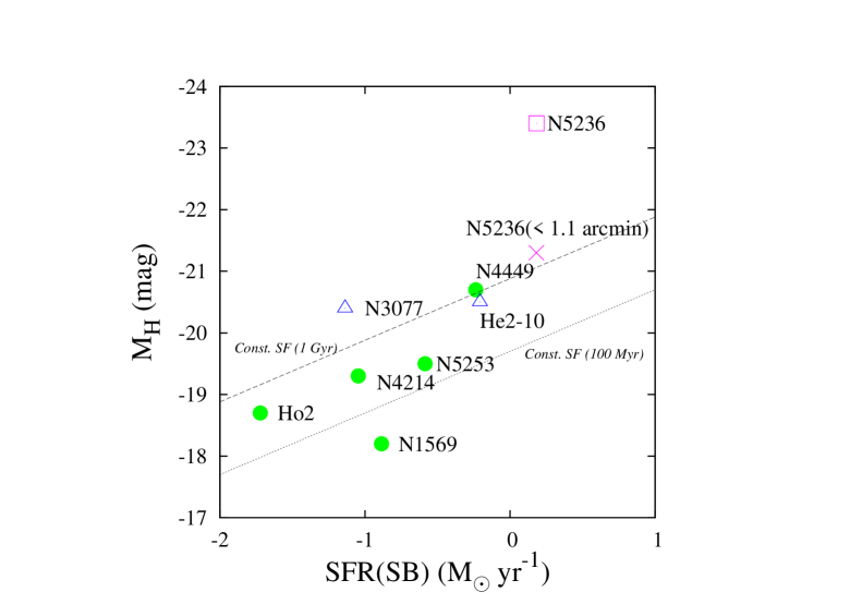
Figure 1.— The H-band luminosity from 2MASS (a proxy of stellar mass; Jarrett et al. 2003) vs. SFR for starburst region (SB), shown in Figure 10, for the sample grouped by metal abundance; sub-solar (solid circle), solar (open triangle), and super-solar (open square). The dotted and dashed lines show the H-band magnitudes derived from STARBURST99 for constant star forming history with the given period of time; 100 Myr (dot) and 1 Gyr (dash). Because NGC 5236 is a large spiral galaxy, we also put the H-band magnitude with the aperture size of 1.1 arcmin (Jarrett et al. 2003), which is matched to the size of the central starburst region.

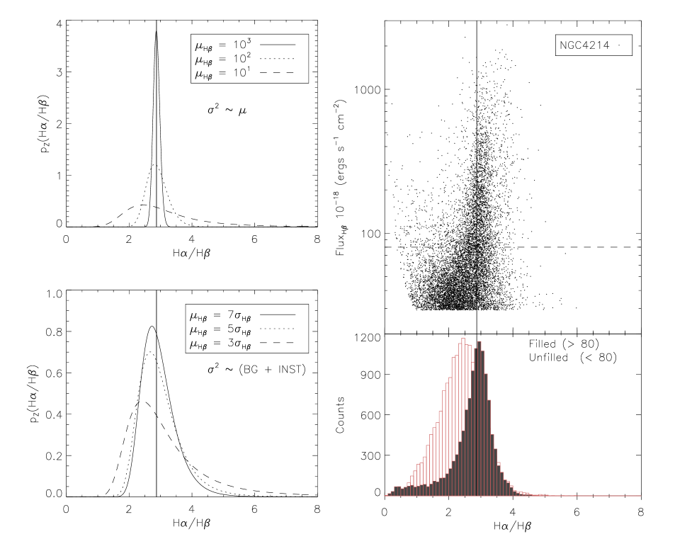
Figure 2.— The probability density functions of H$\alpha$/H$\beta~{}$ratio for zero extinction, i.e. the intrinsic H$\alpha$/H$\beta~{}$= 2.87, from Equation 2 for various variances (left panels). For a bright source, the noise is dominated by the Poisson fluctuations on the source counts. The left-top panel represents this source-dominated case, while the left-bottom panel is for a background and instrument (BG+INST) noise-dominated case. The observed H$\alpha$/H$\beta~{}$ratio versus the H$\beta~{}$flux for NGC 4214 (right-top panel) and its number count histograms (right-bottom panel). The vertical lines represent the positions of H$\alpha$/H$\beta~{}$= 2.87. The horizontal dashed line on the right-top panel shows the threshold line where the H$\beta~{}$flux is equal to 80 in the given scale unit. Above the threshold line (the filled histogram in the right-bottom panel), the signal is relatively strong, hence the broadening caused by statistical measurement error is relatively small as shown in the left-top panel (the probability function for $\mu_{H\beta}=10^{3}$). Below the threshold (the unfilled histogram in the right-bottom panel), the statistical broadening becomes larger. Even though we consider other factors affecting the observed ratios, such as real dust extinction and residuals from stellar continuum subtraction, the statistical broadening shows a significant impact on the observed ratios. This statistical bias can propagate during dust extinction correction.

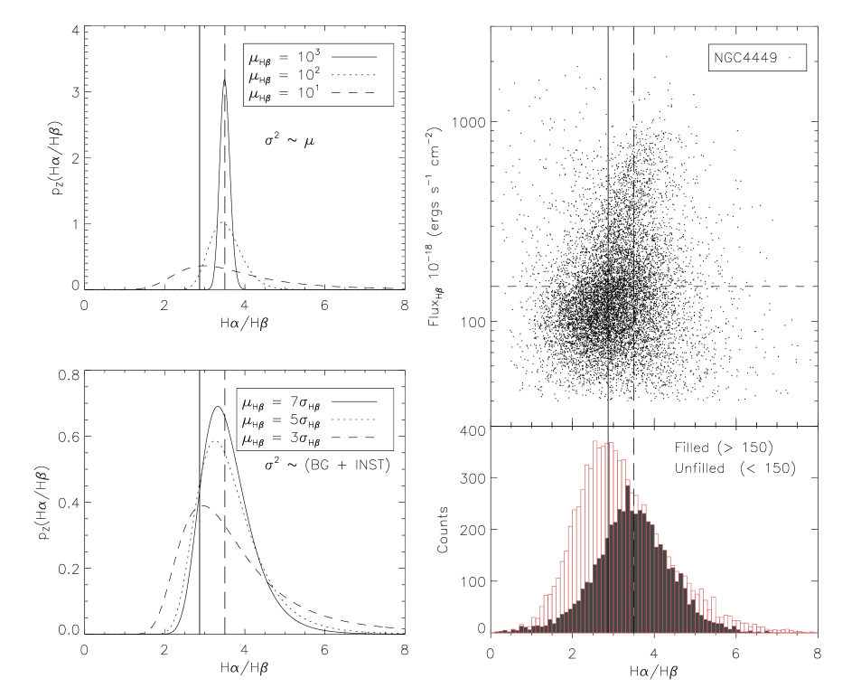
Figure 3.— The same figure with Figure 2 for NGC 4449. Here we set the intrinsic ratio as H$\alpha$/H$\beta~{}$=3.5 corresponding to E(B$-$V) = 0.2, which is the centroid of the filled histogram in the right-bottom panel. Due to the different depth of observation for NGC 4449, we set the threshold line at 150 in the given scale unit. The solid vertical lines represent the ratio, H$\alpha$/H$\beta~{}$=2.87, the same with Figure 2 and the long-dashed vertical lines the ratio, H$\alpha$/H$\beta~{}$=3.5. The probability functions (left panels) look similar with the ones in Figure 2, but they become broader. When we average out the histogram for dust extinction, the statistical bias can be alleviated. Therefore, galaxy-averaged correction can suffer less from this bias. But for pixel-by-pixel correction, especially that E(B$-$V) is set to zero when H$\alpha$/H$\beta~{}$$<2.87$, the corrected line flux is typically overestimated due to this statistical broadening issue.

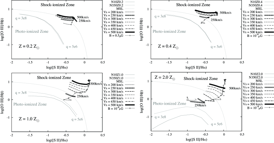
Figure 4.— Tracks of the photo-ionization models (Kewley et al. 2001) and the shock–ionization models (Allen et al. 2008) for the metallicities, $0.2Z_{\odot}$, $0.4Z_{\odot}$, $1.0Z_{\odot}$, and $2.0Z_{\odot}$. The MSL is the “maximum starburst line” in Kewley et al. (2001). The tracks’ location depends on metallicity, especially for the photoionized gas. N10Z0.2 represents the photoionization model for the ISM density, 10 $cm^{-3}$, and the metallicity, $Z=0.2Z_{\odot}$; and the other photoionization models are named in the same way with N10Z0.2. For shock models, the lines of $B=0.5\mu G$ and $10^{-4}\mu G$ are the main branches showing the velocity dependence of shock–ionization grids. The side branches of given shock velocity $V_{s}$ show the magnetic field effects. We use $B=0.5\mu G$ models for $Z=0.2Z_{\odot}$ instead of $B=10^{-4}\mu G$, because the solutions do not converge in low metallicity and magnetic field. The density of preshock gas is 1 $cm^{-3}$.

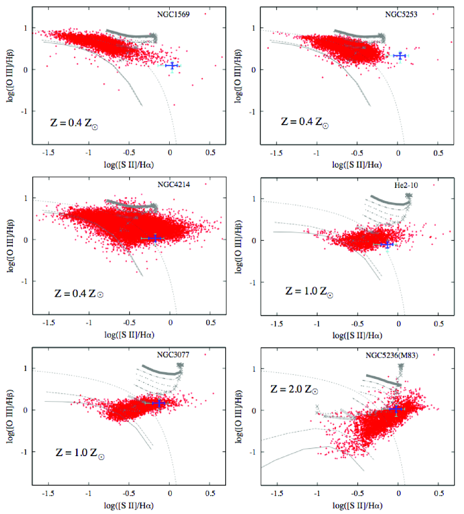
Figure 5.— The [S ii] diagnostic diagram for each galaxy with theoretical grids. The grey lines show the theoretical grids presented in Figure 4. The error bars are presented at MUR spots; thin (cyan) error bars for $5\sigma$ detections and thick (blue) error bars for $10\sigma$ detections.

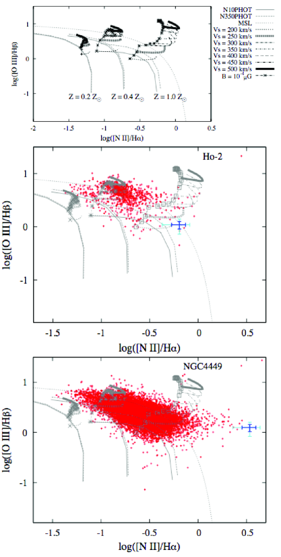
Figure 6.— Theoretical grids for the [N ii] diagnostics like Figure 4 (top). We plot all the models with the three metallicities, $Z=0.2,0.4,1.0Z_{\odot}$, in this single panel. The same error bars as presented in Figure 5. Diagnostic diagrams for Holmberg II (middle) and NGC 4449 (bottom) with theoretical tracks presented on the top panel. The [N ii] diagnostics shows the clear separation between different metallicities, but more overlaps between shock– and photo–ionization grids than the [S ii] diagnostics.

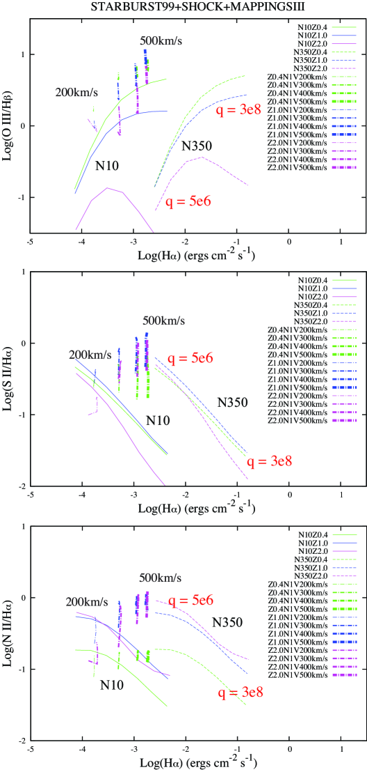
Figure 7.— The line ratio of [O III]($\lambda$5007)/H$\beta~{}$([S II]($\lambda\lambda$6716,6731)/H$\alpha$, [N II]($\lambda$6583)/H$\alpha$) as a function of the normalized H$\alpha~{}$from K01 and A08. The models are the same ones presented in Figure 4 and Figure 6. We plot the grids with different colors for each metallicity; $Z=0.4Z_{\odot}$ in green, $Z=1.0Z_{\odot}$ in blue, and $Z=2.0Z_{\odot}$ in magenta. The N350 photoionization models are located on the right-hand side of the N10 models due to their higher density; so stronger H$\alpha~{}$emission. The shock–ionized gas has generally higher line ratios shown as vertical lines in the plots for all of the three line ratios than photo–ionized gas. This property can be used as a shock separator, using $\log$([S II]($\lambda\lambda$6716,6731)/H$\alpha$$)>-0.5$. We can also find that the [O III]($\lambda$5007)/H$\beta~{}$ratios in H$\alpha~{}$bright regions show a strong metallicity dependence as previously shown in Figure 4.

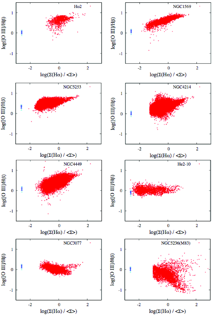
Figure 8.— The line ratio of [O III]($\lambda$5007)/H$\beta~{}$as a function of the normalized H$\alpha~{}$surface brightness with the error bars presented in Figure 5. The surface brightness is normalized to the half-light radius surface brightness $<\Sigma>$; i.e. the sum of all pixels over this value is equal to the half of the total H$\alpha~{}$flux. The metallicity dependence of [O III]($\lambda$5007)/ṟatios in the bright end of H$\alpha~{}$flux fits well with the theoretical grids shown in the top panel of Figure 7. We can recognize the three groups from the figures; the sub-solar group(NGC 1569, NGC 5253, NGC 4449, Holmberg II, NGC 4214), the solar group (He 2-10, NGC 3077), and the super-solar groups (NGC 5236). Due to the dust lanes in NGC 5236, the horizontal pixel distribution near [O III]($\lambda$5007)/H$\beta~{}$$\approx 0.0$ is a propagated error from dust extinction correction.

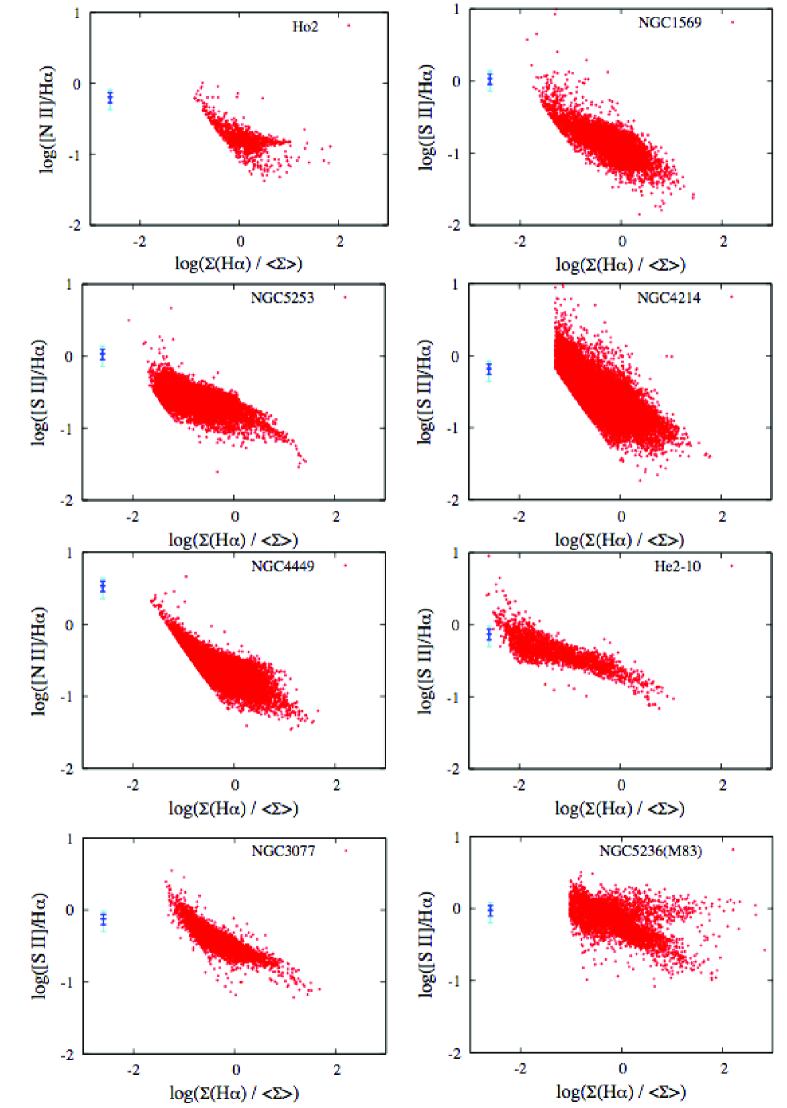
Figure 9.— The line ratio of [S II]($\lambda\lambda$6716,6731)/H$\alpha~{}$(and [N II]($\lambda$6583)/H$\alpha~{}$for Holmberg II and NGC 4449) as a function of the normalized H$\alpha~{}$surface brightness with the error bars presented in Figure 5. We can use this ratio for shock separation, such as $\log($[S II]($\lambda\lambda$6716,6731)/H$\alpha$$)>-0.5$, though the estimated shock is less reliable than the estimates from the diagnostic diagrams, because of the potential contamination from hot, diffuse photo–ionized gas.

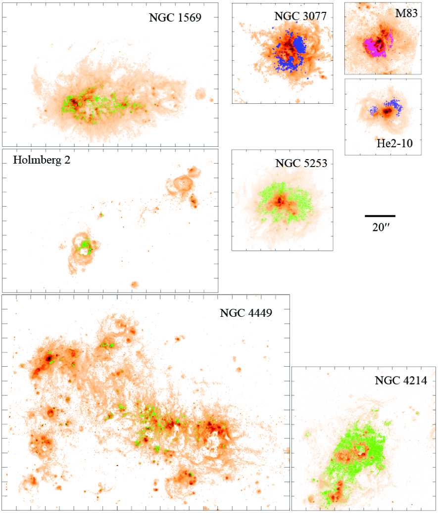
Figure 10.— Distribution of identified shocks over the H$\alpha~{}$images (painted in green for sub-solar sample, blue for solar sample, and magenta for super-solar sample). Most identified shocks are located in the outer rim from the central or most prominent starburst.

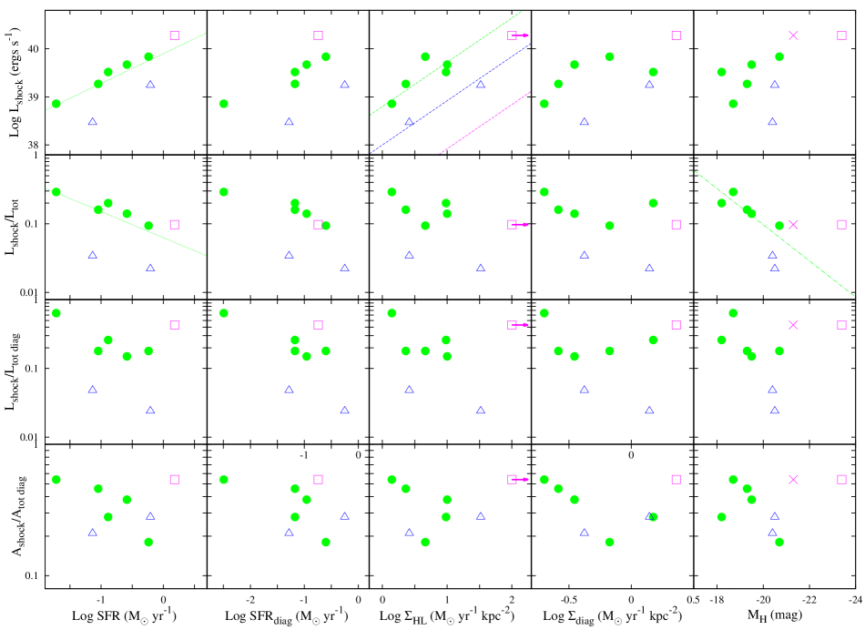
Figure 11.— Relations between star formation rate (or density), absolute H-band magnitude, and shock–ionized gas properties presented in Table 4. The “diag” quantities, biased measurements depending on detection threshold, do not show any better relation than the other quantities. We ignore the relations connected with the “diag” quantities. The shock H$\alpha~{}$luminosity, $L_{shock}$, correlates with both SFR and SFR density, $\Sigma_{SFR,HL}$; the shock ratio, $L_{shock}/L_{tot}$, correlates with $M_{H}$. The green lines represent the relations presented in Equations 3 – 6. The blue and magenta dashed lines on the panel of $L_{shock}$ vs. $\Sigma_{SFR,HL}$ show the magnitude of the offset to be applied to the green dashed line as a consquence of effects that lead to the underestimate of $L_{shock}$ (use of the MSL) and the increase of $\Sigma_{SFR,HL}$ (more compact emitting regions) in more metal rich galaxies. A smaller metallicity effect is observed in the $L_{shock}$ vs. SFR relation, because the SFR is not impacted by the size of the emitting region.

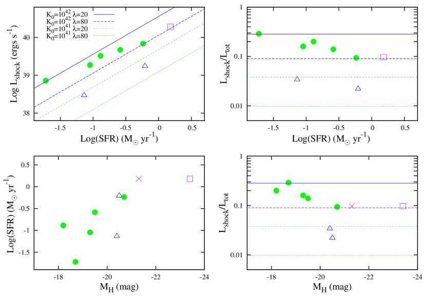
Figure 12.— Relations between SFR – $L_{sh}$(top-left), SFR – $L_{sh}/L_{tot}$(top-right), $M_{H}$ – SFR(bottom-right), and $M_{H}$ – $L_{sh}/L_{tot}$(bottom-right), presented in Figure 1 and Figure 11. Due to SFR$=\kappa L_{tot}$, the two top panels are equivalent. The lines represent the theoretical ratio $\mu/(1+\mu)$, where $\mu=\kappa K_{0}/\lambda$ in Equation 19 and 20. The range of $\mu$ can cover the observed data. Because $M_{H}$ – SFR is not independent (Noeske et al. 2007), the relations on the right panels are projected results from the underlying 3 dimensional relation of $L_{sh}/L_{tot}\sim(M_{H},$SFR). The bottom-right panel of Figure 13 shows the preliminary 3 dimensional relation.

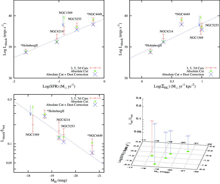
Figure 13.— Corrections to $L_{shock}$: apparent thresholds, $3\sigma$, $5\sigma$, and $7\sigma$ (red bar), absolute threshold (green point), and dust correction to the line ratios (blue point). The dashed lines represent $L_{shock}\propto SFR^{0.62\pm 0.05}$, $L_{shock}\propto{\Sigma_{SFR,HL}}^{0.92\pm 0.41}$, and $L_{shock}/L_{tot}\propto{10}^{0.26(\pm 0.08)M_{H}}$ (or $\propto{(L_{H}/L_{H,\odot})}^{-0.65\pm 0.2}$). Homlemberg II and NGC 4449 are marked with asterisk (*) to indicate their uses of the [N ii] diagnostics, while the others of the [S ii] diagnostics. From the red bars, we can find that non-negligible amount of shocks can be found from a deeper observation. NGC 1569 is indicated as an arrow because the absolute cut corresponds to 1 – 2 sigma levels for the line emission images. Due to the heavy dust extinctions of NGC 1569, the dust correction should be significant for NGC 1569. We mark the dust correction effect as a blue arrow, which works in the opposite direction of the absolute cut effect. NGC 4449 and NGC 5253 turn out to have significant dust corrections (see the green and blue points). Though we have limited number statistics, this figure shows a strong evidence for the existence of regulations between the four quantities, $L_{shock}$, $L_{shock}/L_{tot}$, SFR, and $M_{H}$. The bottom-right panel shows the three dimensional plot of $L_{shock}/L_{tot}$ vs. M_H and SFR. The four blue points are the same blue points on the other panels for NGC 4449, NGC 5253, NGC 4214, and Holmberg II. NGC 1569 is plotted in red with its 5$\sigma$ cut result. The sub-linear scaling of $L_{shock}\propto SFR^{0.62\pm 0.05}$ can be due to projection effects of the three dimensional relation.

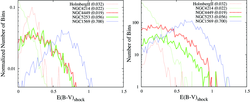
Figure 14.— The dust extinction, E(B–V), applied to shock–ionized bins. The right panel shows the absolute counts of the shock–ionized bins to which dust correction is applied and the left panel the normalized counts. Holmberg II and NGC 4214 show small dust extinction, while NGC 1569 shows very high E(B–V) due to its heavy foreground extinction. The dust extinction correction are not negligible in NGC 5253, NGC 4449 and NGC 1569. NGC 5253 and NGC 4449 show similar distributions of E(B–V) in the left panel. But, in the right panel, we find that NGC 4449 has more pixel bins than NGC 5253. Due to this, as described in §4.2.2, the dust correction affects proportionally more NGC 4449 than NGC 5253.

References

- (1) Allen, M.G., et al. 2008, ApJS 178, 20 (A08)
- (2) Baldwin, J. A., Philips, M. M., & Terlevich, R. 1981, PASP, 93, 5
- (3) Berg, D. A., et al. 2012, ApJ, 754, 98
- (4) Bresolin, F., et al. 2005, A&A, 441, 981
- (5) Bresolin, F. 2011, ApJ, 729, 56
- (6) Croxall, K. V., et al. 2009, ApJ, 705, 723
- (7) Binette, L., Dopita, M. A., & Tuohy, I. R. 1985, ApJ, 297, 476
- (8) Calzetti, D., Harris, J., Gallagher, J. S., et al. 2004, AJ, 127, 1405 (C04)
- (9) Cardelli, J. A., Clayton, G. C., & Mathis, J. S. 1989. ApJ, 345, 245
- (10) Cecil, G., Bland-Hawthorn, J., & Veilleux, S. 2002, ApJ 576, 745
- (11) Chandar, R., et al. 2010, ApJ, 719, 966
- (12) Chevalier, R. A., & Clegg, A.W. 1985, Nature 317, 44
- (13) Davé, R., Oppenheimer, B. D., & Finlator, K. 2011, MNRAS, 415, 11
- (14) De Young, D.S., & Heckman, T.M. 1994, ApJ 431, 598
- (15) Engelbracht, C. W., et al. 2008, ApJ, 678, 804
- (16) Fruchter, A., et al. 2009, ”The MultiDrizzle Handbook”, version 3.0, (Baltimore, STScI)
- (17) Gonzaga, S., & Biretta, J., et al. 2010, in HST WFPC2 Data Handbook, v. 5.0, ed., (Baltimore, STScI)
- (18) Guseva, N. G., et al. 2011, A&A, 529, A149
- (19) Heckman, T.M., Armus, L., & Miley, G.K. 1990, ApJS, 74, 833
- (20) Hinkley, D. V. 1969, Biometrika, 56, 635
- (21) Hong, S., et al. 2010, arXiv:1008.4242v2
- (22) Hong, S., et al. 2011, ApJ, 731, 45 (H11)
- (23) Hong, S., et al. 2013 in prep.
- (24) Hopkins, P. F., Quataert, E., & Murray, N. 2012. MNRAS, 421, 3522 (HQM)
- (25) Jarrett, T. H., Chester, T., Cutri, R., Schneider, S. E., & Huchra, J. P. 2003. ApJ, 125, 525
- (26) Kauffmann, G., et al. 2003, MNRAS, 346, 1055
- (27) Kennicutt, R. C. 1998, ARA&A, 36, 189
- (28) Kennicutt, R. C. 1998, ApJ, 498, 541
- (29) Kennicutt, R. C. et al. 2008, ApJS, 178, 247
- (30) Kobulnicky, H. A., & Skillman, E. D. 1996, ApJ, 471, 211
- (31) Kobulnicky, H. A., et al. 1997, ApJ, 477, 679
- (32) Kobulnicky, H. A., & Skillman, E. D. 1997, ApJ, 489, 636
- (33) Kobulnicky, H. A., et al. 1999, ApJ, 514, 544
- (34) Kewley, L. J., et al. 2001, ApJ, 556, 121(K01)
- (35) Kewley, L.J., & Dopita, M.A. 2002, ApJS, 142, 35
- (36) Leitherer, C., et al. 1999, ApJS, 123, 3
- (37) Lejeune, Th., Cuisinier, F., & Buser, R. 1997, A&AS, 125, 229
- (38) MacLow, M.-M., McCray, R., & Norman, M. L. 1989, ApJ, 337, 141
- (39) MacLow, M.-M., & Ferrara, A. 1999, ApJ, 513, 142
- (40) Martin, C.L. 1997, ApJ, 491, 561
- (41) Martin, C.L., Kobulnicky, H.A., & Heckman, T.M. 2002, ApJ, 574, 663
- (42) Mustakas, J. et al. 2010, ApJS, 190, 233
- (43) Nava, A., et al. 2006, ApJ, 645, 1076
- (44) Noeske, K. G. et al. 2007, ApJ, 660, L43
- (45) Oppenheimer, B.D, & Davé, R.2006, MNRAS, 373, 1265
- (46) Pilyugin, L. S., Vílchez, J. M., & Contini, T. 2004, A&A, 425, 849
- Reynolds et al. (1999) Reynolds, R. J., Haffner, L. M., & Tufte, S. L. 1999, ApJ, 525, L21
- Reynolds et al. (2001) Reynolds, R. J., Sterling, N. C., Haffner, L. M., & Tufte, S. L. 2001, ApJ, 548, L221
- (49) Rich, J. A. et al. 2010, ApJ, 721, 505
- (50) Teukolsky, et al. 1992, “Numerical Recipes The Art of Scientific Computing: Second Edition”, Cambridge Press
- (51) Tremonti, C.A., et al. 2004, ApJ, 613, 898
- (52) Scannapieco, C., Tissera, P.B., White, S.D.M., & Springel, V. 2008, MNRAS, 389, 1137
- (53) Schaller, G., Schaerer, D., Meynet, G., & Maeder, A. 1992, A&AS, 96, 269
- (54) Silich, S., Tenorio-Tagle, G., & Munon-Tunon, C. 2003, ApJ 590, 791
- (55) Kurt T. Soto, C. L. Martin, M. K. M. Prescott, and L. Armus 2012, ApJ, 757, 86
- (56) Strickland, D.K., & Stevens, I.R. 2000, MNRAS 314, 511
- (57) Strickland, D.K., et al. 2004, ApJ 606, 829
- (58) Suchkov, A.A., et al. 1996, ApJ, 463, 528
- (59) Sutherland, R. S., & Dopita, M. A. 1993, ApJS, 88, 253