A new method to measure galaxy bias

Jennifer E. Pollack1, Robert E. Smith2,3, & Cristiano Porciani1
1Argelander Institut fΓΌr Astronomie der UniversitΓ€t Bonn, Auf dem HΓΌgel 71, D-53121 Bonn, Germany
2Max-Planck Institute for Astrophysics, Karl-Schwarzschild-Str.1, Postfach 1523, 85740 Garching, Germany
3Astronomy Centre, Department of Physics and Astronomy, University of Sussex, Brighton BN1 9QH
E-mail: jpollack@astro.uni-bonn.deres@mpa-garching.mpg.deporciani@astro.uni-bonn.de
Abstract

We present a new approach for modelling galaxy/halo bias that utilizes the full non-linear information contained in the moments of the matter density field, which we derive using a set of numerical simulations. Although our method is general, we perform a case study based on the local Eulerian bias scheme truncated to second-order. Using 200 N𝑁N-body simulations covering a total comoving volume of 675​hβˆ’3​Gpc3675superscriptβ„Ž3superscriptGpc3675\,h^{-3}\,{\rm Gpc}^{3}, we measure several 222- and 333-point statistics of the halo distribution to unprecedented accuracy. We use the bias model to fit the halo-halo power spectrum, the halo-matter cross spectrum and the corresponding three bispectra for wavenumbers in the range 0.04≲k≲0.12​h​Mpcβˆ’1less-than-or-similar-to0.04π‘˜less-than-or-similar-to0.12β„ŽsuperscriptMpc10.04\lesssim k\lesssim 0.12\,h\,{\rm Mpc}^{-1}. We find the constraints on the bias parameters obtained using the full non-linear information differ significantly from those derived using standard perturbation theory at leading order. Hence, neglecting the full non-linear information leads to biased results for this particular scale range. We also test the validity of the second-order Eulerian local biasing scheme by comparing the parameter constraints derived from different statistics. Analysis of the halo-matter cross-correlation coefficients defined for the 2- and 3-point statistics reveals further inconsistencies contained in the second-order Eulerian bias scheme, suggesting it is too simple a model to describe halo bias with high accuracy.

keywords:
cosmology: theory, large-scale structure

1 Introduction

The clustering statistics of the galaxy distribution contain a wealth of information about the cosmological model. However, in the absence of a robust theory for galaxy formation, extracting this information can only be achieved in part. In practice, to do this requires us to assume a specific phenomenological relationship between the density field of galaxies and that of the underlying matter, more commonly referred to as galaxy bias. Whilst still incomplete, our leading theories of galaxy formation, do provide a great deal of insight about the distribution of galaxies. For instance they predict that galaxies should only reside in dark-matter haloes and be strongly associated with the distribution of sub-structures (for a detailed review of galaxy formation see Mo, van den Bosch & White, 2010). This greatly simplifies our ability to construct a phenomenological model for the galaxy distribution on large scales: it should be closely related to a weighted average of the dark-matter-halo overdensities (e.g. Smith, Scoccimarro & Sheth, 2007).

There are a number of detailed analytical approaches for characterizing the bias of dark-matter haloes with respect to the mass distribution (for a recent review see Porciani, 2013). However, it has yet to be determined which model provides the most accurate description of galaxy bias. In the simplest method, the local Eulerian bias model (hereafter LEB), one assumes that the overdensities of the biased tracers can be written as some function of the matter-density field at the same location. If both densities are smoothed over the patch scale R𝑅R, then the biased field may be written as a Taylor-series expansion (Fry & Gaztanaga, 1993). If one considers sufficiently large patches, then high-order corrections are guaranteed to be small and the series may be truncated after a finite number of terms.

Halo-clustering predictions of the LEB expressed in terms of standard perturbation theory (hereafter SPT, for a review see Bernardeau etΒ al., 2002) have been examined in numerous works (Scoccimarro etΒ al., 2001; Smith, Scoccimarro & Sheth, 2007; Guo & Jing, 2009; Roth & Porciani, 2011; Manera & GaztaΓ±aga, 2011; Pollack, Smith & Porciani, 2012; Chuen Chan & Scoccimarro, 2012). One of the results to emerge from these studies is that, when the model is applied to halo counts within finite volumes of linear size R𝑅R, the coefficients of the bias expansion show a running with the β€œcell” size. However, halo-clustering statistics such as the n𝑛n-point correlation functions (or the corresponding n𝑛n-spectra) do not contain any smoothing scale and should not depend on R𝑅R. There has been much debate in the literature on how to reconcile these seemingly contrasting results (see Porciani, 2013, for a concise summary).

This has led some to discuss an β€œeffective” or β€œrenormalized” bias approach where the scale-dependence of the bias coefficients is compensated by the contribution of small-scale perturbations in the matter density (Heavens, Matarrese & Verde, 1998; McDonald, 2006; Schmidt, Jeong & Desjacques, 2012). Whilst such a scheme may be plausible (Jeong & Komatsu, 2008; Smith, HernΓ‘ndez-Monteagudo & Seljak, 2009), the development of a unique renormalization method is still ongoing, especially for dynamically evolved configurations in Eulerian space. On the other hand, it was recently proposed by Chuen Chan & Scoccimarro (2012) that the bias parameters obtained counting halos within cells of size R𝑅R are only relevant for describing perturbations of wavenumber k≃0.8/Rsimilar-to-or-equalsπ‘˜0.8𝑅k\simeq 0.8/R in the halo distribution. While there is no challenge to their argument when analyzing power-spectrum data, it does present a complication when using higher-order statistics such as the bispectrum. In order to interpret the galaxy bispectrum one would be required to compute bias coefficients separately for each configuration of wavevectors. This approach appears somewhat cumbersome to implement.

Currently, most observational analyses of galaxy clustering assume that galaxy bias can be described by the truncated LEB and that the statistical properties of the non-linear matter density field can be modelled using SPT. To leading order in the perturbations, this requires only one bias parameter for 2-point statistics of the tracers and two parameters for 3-point statistics. Present-day galaxy surveys, however, do not cover enough comoving volume to accurately sample the spatial scales at which tree-level results provide an accurate description of galaxy clustering. The presence of rare large-scale structures, for instance, significantly alters the measurements of three-point statistics (e.g. Nichol etΒ al., 2006). On smaller scales, where data are more robust, dynamical non-linearities pose a serious challenge to the models. Adopting the simplified LEB+SPT model may therefore generate systematic errors and thus influence the characterisation of the bias or the estimation of the cosmological parameters.

The LEB truncated to second order is the standard workhorse for studying three-point statistics of galaxy clustering. Its predictions to leading perturbative order have been used to interpret measurements from the two-degree field galaxy redshift survey (Verde etΒ al., 2002; Jing & BΓΆrner, 2004; Wang etΒ al., 2004; GaztaΓ±aga etΒ al., 2005), the Sloan Digital Sky Survey (Kayo etΒ al., 2004; Hikage etΒ al., 2005; Pan & Szapudi, 2005; Kulkarni etΒ al., 2007; Nishimichi etΒ al., 2007; MarΓ­n, 2011; McBride etΒ al., 2011, 2011; Guo etΒ al., 2013), and the WiggleZ Dark Energy Survey (MarΓ­n etΒ al., 2013). In our previous study (Pollack, Smith, & Porciani, 2012), we demonstrated that, in order to robustly model three-point statistics with the LEB, one must necessarily have an accurate model for the clustering statistics of the non-linear matter density on the relevant scales. This is imperative to recover the correct values of the bias parameters in controlled numerical experiments. Therefore, it is not surprising that past investigations based on the LEB+SPT model reached inconsistent conclusions. For example, studying the galaxy bispectrum on scales 0.1<k<0.5​h​Mpcβˆ’10.1π‘˜0.5β„ŽsuperscriptMpc10.1<k<0.5\,h\,{\rm Mpc}^{-1}, Verde etΒ al. (2002) concluded that 2dF galaxies are unbiased tracers of the mass distribution. On the other hand, using the complete 2dF sample, GaztaΓ±aga etΒ al. (2005) found strong evidence for non-linear biasing from the analysis of the three-point correlation function with triangle configurations that probe separations between 9 and 36​hβˆ’1​Mpc36superscriptβ„Ž1Mpc36\,h^{-1}{\rm Mpc} (see also Jing & BΓΆrner, 2004; Wang etΒ al., 2004).

In this paper, we build upon our past experience and present a general method to model the clustering of biased tracers of the mass distribution on mildly non-linear scales k<0.1​h​Mpcβˆ’1π‘˜0.1β„ŽsuperscriptMpc1k<0.1\,h\,{\rm Mpc}^{-1}. This is key to extend studies of galaxy clustering to smaller spatial separations where observational data are less uncertain. Our method relies on using N-body simulations to measure the relevant statistics for the clustering of the underlying mass distribution. Related approaches have been presented by Sigad, Branchini & Dekel (2000) and Szapudi & Pan (2004) for galaxy counts in cells (see also Pan & Szapudi, 2005, for an application to correlation functions). We apply our general framework to the modelling of n𝑛n-point clustering statistics of non-linear, Eulerian, locally biased tracers. In our framework, bias parameters run with the patch scale R𝑅R. We address the running of the bias by treating the filter scale as a nuisance parameter to be marginalized over. The major advantage of our scheme is that we exactly recover the matter poly-spectra used in the bias model at every order. The only truncation necessary in the model is the choice as to what level to truncate the bias expansion, and this may be selected by the data in a Bayesian model comparison. We test our modelling framework up to quadratic order in the local bias expansion (as commonly done in recent observational studies), for the power- and bi-spectra of haloes and their cross-spectra with matter measured from a large ensemble (200 realizations) of measurements from a series of large ΛΛ\LambdaCDM N𝑁N-body simulations. This ensemble of simulations resolves the halos that should host luminous red galaxies over a total comoving volume of 675​hβˆ’3​Gpc3675superscriptβ„Ž3superscriptGpc3675\,h^{-3}\,{\rm Gpc}^{3}, and so provides us with a very stringent statistical test ground for our model.

The sections are organized as follows. In Β§2 we set our mathematical notation and introduce the LEB. The numerical simulations used in this work are briefly described in Β§3 and used in Β§4 to measure several statistical quantities for the matter and halo distributions. In Β§5 we use Bayesian statistics to estimate the free parameters of the LEB and describe our main results. Finally, in Β§6 and 7 we further discuss our findings and present our conclusions.

2 A new framework for modelling the clustering of biased tracers

2.1 General formalism

Consider some discrete tracers of the large-scale structure (dark-matter haloes or galaxies) with mean density nΒ―hsubscript¯𝑛h\bar{n}_{\rm h} and physical density ρh​(𝐱)=[1+Ξ΄h​(𝐱)]​nΒ―hsubscript𝜌h𝐱delimited-[]1subscript𝛿h𝐱subscript¯𝑛h\rho_{\rm h}({\bf x})=[1+\delta_{\rm h}({\bf x})]\,\bar{n}_{\rm h}. We want to relate this random field to the underlying distribution of matter with local density ρ​(𝐱)=[1+δ​(𝐱)]β€‹ΟΒ―πœŒπ±delimited-[]1π›Ώπ±Β―πœŒ\rho({\bf x})=[1+\delta({\bf x})]\,\bar{\rho}. If we assume that the density contrast of the tracers averaged over some patch of linear size R𝑅R, Ξ΄h​(𝐱|R)subscript𝛿hconditional𝐱𝑅\delta_{\rm h}({\bf x}|R), is locally related to the density of matter in the same patch, then we may write

Ξ΄h​(𝐱|R)=ℱ​[δ​(𝐱|R)]subscript𝛿hconditional𝐱𝑅ℱdelimited-[]𝛿conditional𝐱𝑅\delta_{\rm h}({\bf x}|R)={\mathcal{F}}\left[\delta({\bf x}|R)\right] (1)

where β„±β„±{\mathcal{F}} denotes a generic function ℝ→ℝ→ℝℝ\mathbb{R}\to\mathbb{R} and the symbols

δα​(𝐱|R)β‰‘βˆ«d3​𝐲​W​(|π±βˆ’π²|,R)​δα​(𝐲)subscript𝛿𝛼conditional𝐱𝑅superscriptd3π²π‘Šπ±π²π‘…subscript𝛿𝛼𝐲\delta_{\alpha}({\bf x}|R)\equiv\int{\rm d}^{3}\!{\bf y}\,W(|{\bf x}-{\bf y}|,R)\,\delta_{\alpha}({\bf y}) (2)

(where α𝛼\alpha stands for haloes or matter) denote smoothed overdensity fields, Wπ‘ŠW being a rotation-invariant filter function with size R𝑅R.

Since we are dealing with smooth mathematical functions we may Taylor expand Eq. (1) to obtain (Fry & Gaztanaga, 1993):

Ξ΄h​(𝐱|R)=βˆ‘n=1∞bnn!​[Ξ΄n​(𝐱|R)βˆ’βŸ¨Ξ΄n​(𝐱|R)⟩],subscript𝛿hconditional𝐱𝑅superscriptsubscript𝑛1subscript𝑏𝑛𝑛delimited-[]superscript𝛿𝑛conditional𝐱𝑅delimited-⟨⟩superscript𝛿𝑛conditional𝐱𝑅\delta_{\rm h}({\bf x}|R)=\sum_{n=1}^{\infty}\frac{b_{n}}{n!}\left[\delta^{n}({\bf x}|R)-\langle\delta^{n}({\bf x}|R)\rangle\right]\ , (3)

where the terms bnsubscript𝑏𝑛b_{n} are the Eulerian bias coefficients of order n𝑛n, which depend on both the smoothing scale and the exact definition of the tracers (e.g. halo mass, etc.). Note that the subtraction of the terms ⟨δn​(𝐱|R)⟩delimited-⟨⟩superscript𝛿𝑛conditional𝐱𝑅\langle\delta^{n}({\bf x}|R)\rangle at each order ensures that ⟨δh​(𝐱|R)⟩=0delimited-⟨⟩subscript𝛿hconditional𝐱𝑅0\langle\delta_{\rm h}({\bf x}|R)\rangle=0, where βŸ¨β€¦βŸ©delimited-βŸ¨βŸ©β€¦\langle\dots\rangle denote an ensemble average. On Fourier transforming the above relation one finds, for |𝐀|β‰ 0𝐀0|{\bf k}|\neq 0,

Ξ΄~h​(𝐀|R)=βˆ‘n=1∞bnn!​Δ(n)​(𝐀|R)subscript~𝛿hconditional𝐀𝑅superscriptsubscript𝑛1subscript𝑏𝑛𝑛superscriptΔ𝑛conditional𝐀𝑅\tilde{\delta}_{\rm h}({\bf k}|R)=\sum_{n=1}^{\infty}\frac{b_{n}}{n!}\,\Delta^{(n)}({\bf k}|R) (4)

where Ξ”(n)​(𝐀|R)≑δn~​(𝐀|R)superscriptΔ𝑛conditional𝐀𝑅~superscript𝛿𝑛conditional𝐀𝑅\Delta^{(n)}({\bf k}|R)\equiv\widetilde{\delta^{n}}({\bf k}|R) can be written as

Ξ”(n)​(𝐀|R)≑(2​π)3β€‹βˆ«Ξ΄D​(π€βˆ’πͺ1​…​n)β€‹βˆi=1nΞ΄~​(πͺi|R)​d3​πͺi(2​π)3.superscriptΔ𝑛conditional𝐀𝑅superscript2πœ‹3superscript𝛿𝐷𝐀subscriptπͺ1…𝑛superscriptsubscriptproduct𝑖1𝑛~𝛿conditionalsubscriptπͺ𝑖𝑅superscriptd3subscriptπͺ𝑖superscript2πœ‹3\Delta^{(n)}({\bf k}|R)\equiv(2\pi)^{3}\int\delta^{D}({\bf k}-{\bf q}_{1\dots n})\,\prod_{i=1}^{n}\,\tilde{\delta}({\bf q}_{i}|R)\,\frac{{\rm d}^{3}{\bf q}_{i}}{(2\pi)^{3}}\;.\ (5)

In the last expression Ξ΄D​(𝐀)superscript𝛿𝐷𝐀\delta^{D}({\bf k}) denotes the Dirac-delta distribution and we have made use of the compact notation πͺ1​…​n=πͺ1+β‹―+πͺnsubscriptπͺ1…𝑛subscriptπͺ1β‹―subscriptπͺ𝑛{\bf q}_{1\dots n}={\bf q}_{1}+\dots+{\bf q}_{n} and Ξ΄~​(πͺ|R)≑δ~​(πͺ)​W~​(q​R)~𝛿conditionalπͺ𝑅~𝛿πͺ~π‘Šπ‘žπ‘…\tilde{\delta}({\bf q}|R)\equiv\tilde{\delta}({\bf q})\,\widetilde{W}(qR).

We now define the power spectrum of the biased tracers and their cross-spectrum with the matter in terms of the correlators:

⟨δ~α​(𝐀1|R)​δ~β​(𝐀2|R)βŸ©β‰‘(2​π)3​δD​(𝐀12)​𝒫α​β​(k1).delimited-⟨⟩subscript~𝛿𝛼conditionalsubscript𝐀1𝑅subscript~𝛿𝛽conditionalsubscript𝐀2𝑅superscript2πœ‹3superscript𝛿𝐷subscript𝐀12subscript𝒫𝛼𝛽subscriptπ‘˜1\langle\tilde{\delta}_{\alpha}({\bf k}_{1}|R)\,\tilde{\delta}_{\beta}({\bf k}_{2}|R)\rangle\equiv(2\pi)^{3}\,\delta^{D}({\bf k}_{12})\,{\mathcal{P}}_{\alpha\beta}(k_{1})\;. (6)

Similarly, the corresponding bispectra can be defined as

⟨δ~α​(𝐀1|R)​δ~β​(𝐀2|R)​δ~γ​(𝐀3|R)⟩delimited-⟨⟩subscript~𝛿𝛼conditionalsubscript𝐀1𝑅subscript~𝛿𝛽conditionalsubscript𝐀2𝑅subscript~𝛿𝛾conditionalsubscript𝐀3𝑅\displaystyle\langle\tilde{\delta}_{\alpha}({\bf k}_{1}|R)\,\tilde{\delta}_{\beta}({\bf k}_{2}|R)\,\tilde{\delta}_{\gamma}({\bf k}_{3}|R)\rangle ≑\displaystyle\!\!\!\!\!\equiv (7)
≑\displaystyle\equiv (2​π)3​δD​(𝐀123)​ℬα​β​γ​(𝐀1,𝐀2)superscript2πœ‹3superscript𝛿𝐷subscript𝐀123subscriptℬ𝛼𝛽𝛾subscript𝐀1subscript𝐀2\displaystyle\!\!\!\!\!\!\!\!\!\!\!\!\!\!\!\!\!\!\!\!\!\!\!\!\!\!\!\!\!\!\!\!\!\!\!\!\!\!\!\!\!\!(2\pi)^{3}\,\delta^{D}({\bf k}_{123})\,{\mathcal{B}}_{\alpha\beta\gamma}({\bf k}_{1},{\bf k}_{2})

where we have suppressed the dependence of the bispectrum on the third wavevector, since the Dirac-delta distribution imposes 𝐀3=βˆ’π€12subscript𝐀3subscript𝐀12{\bf k}_{3}=-{\bf k}_{12}. On inserting Eq. (4) into Eq. (6), we find:

⟨δ~α(𝐀1|R)\displaystyle\langle\tilde{\delta}_{\alpha}({\bf k}_{1}|R)\!\!\!\!\!\!\!\! δ~β(𝐀2|R)⟩=\displaystyle\!\!\!\!\!\!\!\!\tilde{\delta}_{\beta}({\bf k}_{2}|R)\rangle=
=\displaystyle= βˆ‘l,m=1βˆžΞ“lΞ±l!​ΓmΞ²m!β€‹βŸ¨Ξ”(l)​(𝐀1|R)​Δ(m)​(𝐀2|R)⟩.superscriptsubscriptπ‘™π‘š1subscriptsuperscriptΓ𝛼𝑙𝑙subscriptsuperscriptΞ“π›½π‘šπ‘šdelimited-⟨⟩superscriptΔ𝑙conditionalsubscript𝐀1𝑅superscriptΞ”π‘šconditionalsubscript𝐀2𝑅\displaystyle\!\!\!\!\!\sum_{l,m=1}^{\infty}\frac{\Gamma^{\alpha}_{l}}{l!}\frac{\Gamma^{\beta}_{m}}{m!}\langle\Delta^{(l)}({\bf k}_{1}|R)\,\Delta^{(m)}({\bf k}_{2}|R)\rangle\;.

with Ξ“lh=blsuperscriptsubscriptΓ𝑙hsubscript𝑏𝑙\Gamma_{l}^{\rm h}=b_{l} and Ξ“lm=Ξ΄l​1KsuperscriptsubscriptΓ𝑙msuperscriptsubscript𝛿𝑙1K\Gamma_{l}^{\rm m}=\delta_{l1}^{\rm K} (for haloes and matter, respectively) where Ξ΄i​jKsuperscriptsubscript𝛿𝑖𝑗K\delta_{ij}^{\rm K} denotes the Kronecker-delta function. Similarly for Eq. (7) we have:

⟨δ~Ξ±(𝐀1)Ξ΄~Ξ²(𝐀2)\displaystyle\langle\tilde{\delta}_{\alpha}({\bf k}_{1})\,\tilde{\delta}_{\beta}({\bf k}_{2}) Ξ΄~Ξ³(𝐀3)⟩=βˆ‘l,m,n=1βˆžΞ“lΞ±l!Ξ“mΞ²m!Ξ“nΞ³n!Γ—\displaystyle\!\!\!\!\!\!\!\!\!\!\!\!\!\!\!\!\!\tilde{\delta}_{\gamma}({\bf k}_{3})\rangle=\sum_{l,m,n=1}^{\infty}\frac{\Gamma^{\alpha}_{l}}{l!}\frac{\Gamma^{\beta}_{m}}{m!}\frac{\Gamma^{\gamma}_{n}}{n!}\times
Γ—\displaystyle\times βŸ¨Ξ”(l)​(𝐀1|R)​Δ(m)​(𝐀2|R)​Δ(n)​(𝐀3|R)⟩.delimited-⟨⟩superscriptΔ𝑙conditionalsubscript𝐀1𝑅superscriptΞ”π‘šconditionalsubscript𝐀2𝑅superscriptΔ𝑛conditionalsubscript𝐀3𝑅\displaystyle\!\!\!\!\!\langle\Delta^{(l)}({\bf k}_{1}|R)\,\Delta^{(m)}({\bf k}_{2}|R)\,\Delta^{(n)}({\bf k}_{3}|R)\rangle\;.

It is convenient to introduce the functions 𝒫(l,m)subscriptπ’«π‘™π‘š{\mathcal{P}}_{(l,m)} and ℬ(l,m,n)subscriptβ„¬π‘™π‘šπ‘›{\mathcal{B}}_{(l,m,n)} such that

βŸ¨Ξ”(l)​(𝐀1|R)​Δ(m)​(𝐀2|R)⟩=(2​π)3​δD​(𝐀12)​𝒫(l,m)​(𝐀1)delimited-⟨⟩superscriptΔ𝑙conditionalsubscript𝐀1𝑅superscriptΞ”π‘šconditionalsubscript𝐀2𝑅superscript2πœ‹3superscript𝛿𝐷subscript𝐀12subscriptπ’«π‘™π‘šsubscript𝐀1\langle\Delta^{(l)}({\bf k}_{1}|R)\,\Delta^{(m)}({\bf k}_{2}|R)\rangle=(2\pi)^{3}\,\delta^{D}({\bf k}_{12})\,{\mathcal{P}}_{(l,m)}({\bf k}_{1})\;\, (10)

and

βŸ¨Ξ”(l)​(𝐀1|R)​Δ(m)​(𝐀2|R)​Δ(n)​(𝐀3|R)⟩delimited-⟨⟩superscriptΔ𝑙conditionalsubscript𝐀1𝑅superscriptΞ”π‘šconditionalsubscript𝐀2𝑅superscriptΔ𝑛conditionalsubscript𝐀3𝑅\displaystyle\langle\Delta^{(l)}({\bf k}_{1}|R)\,\Delta^{(m)}({\bf k}_{2}|R)\,\Delta^{(n)}({\bf k}_{3}|R)\rangle =\displaystyle\!\!\!\!\!= (11)
=\displaystyle= (2​π)3​δD​(𝐀123)​ℬ(l,m,n)​(𝐀1,𝐀2)superscript2πœ‹3superscript𝛿𝐷subscript𝐀123subscriptβ„¬π‘™π‘šπ‘›subscript𝐀1subscript𝐀2\displaystyle\!\!\!\!\!\!\!\!\!\!\!\!\!\!\!\!\!\!\!\!\!\!\!\!\!\!\!\!\!\!\!\!\!\!\!\!\!\!\!\!\!\!\!\!\!\!\!\!\!\!(2\pi)^{3}\,\delta^{D}({\bf k}_{123})\,{\mathcal{B}}_{(l,m,n)}({\bf k}_{1},{\bf k}_{2})

In simple words, 𝒫(l,m)subscriptπ’«π‘™π‘š{\mathcal{P}}_{(l,m)} denotes the cross power spectrum between the smoothed random fields [δ​(𝐱|R)]lβˆ’βŸ¨[δ​(𝐱|r)]l⟩superscriptdelimited-[]𝛿conditional𝐱𝑅𝑙delimited-⟨⟩superscriptdelimited-[]𝛿conditionalπ±π‘Ÿπ‘™[\delta({\bf x}|R)]^{l}-\langle[\delta({\bf x}|r)]^{l}\rangle and [δ​(𝐱|R)]mβˆ’βŸ¨[δ​(𝐱|R)]m⟩superscriptdelimited-[]𝛿conditionalπ±π‘…π‘šdelimited-⟨⟩superscriptdelimited-[]𝛿conditionalπ±π‘…π‘š[\delta({\bf x}|R)]^{m}-\langle[\delta({\bf x}|R)]^{m}\rangle, while ℬ(l,m,n)subscriptβ„¬π‘™π‘šπ‘›{\mathcal{B}}_{(l,m,n)} is the corresponding bispectrum. Thus for the halo and matter power and bispectra we have:

𝒫α​β​(𝐀1)subscript𝒫𝛼𝛽subscript𝐀1\displaystyle{\mathcal{P}}_{\alpha\beta}({\bf k}_{1}) =\displaystyle= βˆ‘l,m=1βˆžΞ“lΞ±l!​ΓmΞ²m!​𝒫(l,m)​(𝐀1),superscriptsubscriptπ‘™π‘š1subscriptsuperscriptΓ𝛼𝑙𝑙subscriptsuperscriptΞ“π›½π‘šπ‘šsubscriptπ’«π‘™π‘šsubscript𝐀1\displaystyle\sum_{l,m=1}^{\infty}\frac{\Gamma^{\alpha}_{l}}{l!}\frac{\Gamma^{\beta}_{m}}{m!}\,{\mathcal{P}}_{(l,m)}({\bf k}_{1})\;, (12)
ℬα​β​γ​(𝐀1,𝐀2)subscriptℬ𝛼𝛽𝛾subscript𝐀1subscript𝐀2\displaystyle{\mathcal{B}}_{\alpha\beta\gamma}({\bf k}_{1},{\bf k}_{2})\!\!\! =\displaystyle= βˆ‘l,m,n=1βˆžΞ“lΞ±l!​ΓmΞ²m!​ΓnΞ³n!​ℬ(l,m,n)​(𝐀1,𝐀2).superscriptsubscriptπ‘™π‘šπ‘›1subscriptsuperscriptΓ𝛼𝑙𝑙subscriptsuperscriptΞ“π›½π‘šπ‘šsubscriptsuperscriptΓ𝛾𝑛𝑛subscriptβ„¬π‘™π‘šπ‘›subscript𝐀1subscript𝐀2\displaystyle\!\!\!\!\sum_{l,m,n=1}^{\infty}\frac{\Gamma^{\alpha}_{l}}{l!}\frac{\Gamma^{\beta}_{m}}{m!}\frac{\Gamma^{\gamma}_{n}}{n!}\,{\mathcal{B}}_{(l,m,n)}({\bf k}_{1},{\bf k}_{2})\;. (13)

The above sets of equations provide us with models for the power spectra and the bispectra of halo counts in cells of size R𝑅R. However, what we really want to model is the halo 2- and 3-point functions, Pα​βsubscript𝑃𝛼𝛽P_{\alpha\beta} and Bα​β​γsubscript𝐡𝛼𝛽𝛾B_{\alpha\beta\gamma}. We assume that these quantities can be approximately recovered by β€œde-smoothing” 𝒫α​βsubscript𝒫𝛼𝛽{\mathcal{P}}_{\alpha\beta} and ℬα​β​γsubscriptℬ𝛼𝛽𝛾{\mathcal{B}}_{\alpha\beta\gamma} (Smith, Scoccimarro & Sheth, 2007; Smith, Sheth & Scoccimarro, 2008; Sefusatti, 2009):

Pα​β​(𝐀1)subscript𝑃𝛼𝛽subscript𝐀1\displaystyle P_{\alpha\beta}({\bf k}_{1}) =\displaystyle= 𝒫α​β​(𝐀1)W2​(k1​R);subscript𝒫𝛼𝛽subscript𝐀1superscriptπ‘Š2subscriptπ‘˜1𝑅\displaystyle\frac{{\mathcal{P}}_{\alpha\beta}({\bf k}_{1})}{W^{2}(k_{1}R)}\ ; (14)
Bα​β​γ​(𝐀1,𝐀2,𝐀3)subscript𝐡𝛼𝛽𝛾subscript𝐀1subscript𝐀2subscript𝐀3\displaystyle B_{\alpha\beta\gamma}({\bf k}_{1},{\bf k}_{2},{\bf k}_{3}) =\displaystyle= ℬα​β​γ​(𝐀1,𝐀2,𝐀3)W​(k1​R)​W​(k2​R)​W​(k3​R).subscriptℬ𝛼𝛽𝛾subscript𝐀1subscript𝐀2subscript𝐀3π‘Šsubscriptπ‘˜1π‘…π‘Šsubscriptπ‘˜2π‘…π‘Šsubscriptπ‘˜3𝑅\displaystyle\frac{{\mathcal{B}}_{\alpha\beta\gamma}({\bf k}_{1},{\bf k}_{2},{\bf k}_{3})}{W(k_{1}R)W(k_{2}R)W(k_{3}R)}\ .\ (15)

Note that when considering a model of halo bias beyond linear order this operation does not fully remove the dependence of the theory on R𝑅R. In Section 5, we will use the models presented in Eq. (14) and Eq. (15) to fit simulation data. Nevertheless, our choice to β€œde-smooth” the theoretical model is equivalent to analyzing counts in cell data with a smoothed model. This is due to the fact that in Fourier-space the smoothing kernels can be treated as multiplicative factors, which means that if we factorize the expressions by dividing out the product of the window functions the relation between the model and the data still holds. Hence, fitting counts in cells data with a smoothed model is indifferent to analyzing unsmoothed data with a β€œde-smoothed” or factorized model.

The smoothing scale must therefore be considered as a free parameter of the model, and so it must be either determined by fitting a set of data or marginalized over.

In Β§A.1 and Β§A.2 we show how the terms 𝒫(l,m)subscriptπ’«π‘™π‘š{\mathcal{P}}_{(l,m)} and ℬ(l,m,n)subscriptβ„¬π‘™π‘šπ‘›{\mathcal{B}}_{(l,m,n)} are related to the p𝑝p-point matter spectra, where p=l+mπ‘π‘™π‘šp=l+m or p=l+m+nπ‘π‘™π‘šπ‘›p=l+m+n, respectively. In Β§A.3 we prove that the functions 𝒫(l,m)subscriptπ’«π‘™π‘š{\mathcal{P}}_{(l,m)} are totally symmetric in l𝑙l and mπ‘šm. For lβ‰ mβ‰ nπ‘™π‘šπ‘›l\neq m\neq n, the functions ℬ(l,m,n)​(𝐀1,𝐀2,𝐀3)subscriptβ„¬π‘™π‘šπ‘›subscript𝐀1subscript𝐀2subscript𝐀3{\mathcal{B}}_{(l,m,n)}({\bf k}_{1},{\bf k}_{2},{\bf k}_{3}) are not in general symmetric in l𝑙l, mπ‘šm, and n𝑛n, unless the wavevectors 𝐀isubscript𝐀𝑖{\bf k}_{i} are also exchanged, i.e. whilst ℬ(l,m,n)​(𝐀1,𝐀2,𝐀3)=ℬ(m,l,n)​(𝐀2,𝐀1,𝐀3)subscriptβ„¬π‘™π‘šπ‘›subscript𝐀1subscript𝐀2subscript𝐀3subscriptβ„¬π‘šπ‘™π‘›subscript𝐀2subscript𝐀1subscript𝐀3{\mathcal{B}}_{(l,m,n)}({\bf k}_{1},{\bf k}_{2},{\bf k}_{3})={\mathcal{B}}_{(m,l,n)}({\bf k}_{2},{\bf k}_{1},{\bf k}_{3}), ℬ(l,m,n)​(𝐀1,𝐀2,𝐀3)≠ℬ(m,l,n)​(𝐀1,𝐀2,𝐀3)subscriptβ„¬π‘™π‘šπ‘›subscript𝐀1subscript𝐀2subscript𝐀3subscriptβ„¬π‘šπ‘™π‘›subscript𝐀1subscript𝐀2subscript𝐀3{\mathcal{B}}_{(l,m,n)}({\bf k}_{1},{\bf k}_{2},{\bf k}_{3})\neq{\mathcal{B}}_{(m,l,n)}({\bf k}_{1},{\bf k}_{2},{\bf k}_{3}). Note that in this study we choose to work with n𝑛n-point spectra, 𝒫(Ξ±1​…​αn)subscript𝒫subscript𝛼1…subscript𝛼𝑛{\mathcal{P}}_{(\alpha_{1}\dots\alpha_{n})}, that are symmetric to an exchange of their vectorial arguments, and we accomplish this through the symmetrization operation:

𝒫(Ξ±1​…​αn)(s)=βˆ‘i1,…,inn|Ο΅i1​…​in|​𝒫(Ξ±1​…​αn)​(𝐀i1,…,𝐀in)βˆ‘i1,…,inn|Ο΅i1​…​in|,subscriptsuperscript𝒫ssubscript𝛼1…subscript𝛼𝑛superscriptsubscriptsubscript𝑖1…subscript𝑖𝑛𝑛subscriptitalic-Ο΅subscript𝑖1…subscript𝑖𝑛subscript𝒫subscript𝛼1…subscript𝛼𝑛subscript𝐀subscript𝑖1…subscript𝐀subscript𝑖𝑛subscriptsuperscript𝑛subscript𝑖1…subscript𝑖𝑛subscriptitalic-Ο΅subscript𝑖1…subscript𝑖𝑛{\mathcal{P}}^{\rm(s)}_{(\alpha_{1}\dots\alpha_{n})}=\frac{\sum_{i_{1},\dots,i_{n}}^{n}|\epsilon_{i_{1}\dots i_{n}}|\,{\mathcal{P}}_{(\alpha_{1}\dots\alpha_{n})}({\bf k}_{i_{1}},\dots,{\bf k}_{i_{n}})}{\sum^{n}_{i_{1},\dots,i_{n}}|\epsilon_{i_{1}\dots i_{n}}|}, (16)

where Ο΅i1​…​insubscriptitalic-Ο΅subscript𝑖1…subscript𝑖𝑛\epsilon_{i_{1}\dots i_{n}} denotes the n𝑛n-dimensional generalization of the Levi-Civita symbol and we take its absolute value.

In previous studies, the functions 𝒫(l,m)subscriptπ’«π‘™π‘š{\mathcal{P}}_{(l,m)} and ℬ(l,m,n)subscriptβ„¬π‘™π‘šπ‘›{\mathcal{B}}_{(l,m,n)} have been modelled through the use of a combination of perturbation theory and semi-empirical models. In Pollack, Smith & Porciani (2012) we recovered these functions exactly from an N𝑁N-body simulation and demonstrated that they are essential to measure the bias parameters in an unbiased way. We will revisit these issues in Β§4 and Β§5.

2.2 Case study: biasing to second order

As an example, let us evaluate the case when the bias is taken to second order and all higher-order bias coefficients are vanishing. This is a widespread assumption often used to interpret observational data from massive redshift surveys (see Β§1 for a long list of references). We will consider a unique set of dark-matter haloes. For the case where we have multiple halo bins (e.g. mass selected), the expressions are more cumbersome but no more complicated. Starting with the two-point statistics, one can formulate the halo auto- and cross-power spectra with the total mass up to second-order in the LEB:

𝒫hm​(𝐀)subscript𝒫hm𝐀\displaystyle\mathcal{P}_{\rm hm}({\bf k}) =\displaystyle= b1​𝒫(1,1)​(𝐀)+b22​𝒫(2,1)​(𝐀),subscript𝑏1subscript𝒫11𝐀subscript𝑏22subscript𝒫21𝐀\displaystyle b_{1}\mathcal{P}_{(1,1)}({\bf k})+\frac{b_{2}}{2}{\mathcal{P}}_{(2,1)}({\bf k})\;, (17)
𝒫hh​(𝐀)subscript𝒫hh𝐀\displaystyle\mathcal{P}_{\rm hh}({\bf k}) =\displaystyle= b12​𝒫(1,1)​(𝐀)+b1​b2​𝒫(2,1)​(𝐀)+b224​𝒫(2,2)​(𝐀),superscriptsubscript𝑏12subscript𝒫11𝐀subscript𝑏1subscript𝑏2subscript𝒫21𝐀superscriptsubscript𝑏224subscript𝒫22𝐀\displaystyle b_{1}^{2}\mathcal{P}_{(1,1)}({\bf k})+b_{1}b_{2}{\mathcal{P}}_{(2,1)}({\bf k})+\frac{b_{2}^{2}}{4}\mathcal{P}_{(2,2)}({\bf k})\;,

where from Β§A.1, we see that

𝒫(2,1)​(𝐀)subscript𝒫21𝐀\displaystyle\mathcal{P}_{(2,1)}({\bf k})\!\! ≑\displaystyle\equiv ∫d3​πͺ(2​π)3​ℬ​(πͺ,π€βˆ’πͺ,βˆ’π€),superscriptd3πͺsuperscript2πœ‹3ℬπͺ𝐀πͺ𝐀\displaystyle\!\!\int\frac{{\rm d}^{3}{\bf q}}{(2\pi)^{3}}\,\mathcal{B}({\bf q},{\bf k}-{\bf q},-{\bf k})\;, (19)
𝒫(2,2)​(𝐀)subscript𝒫22𝐀\displaystyle\mathcal{P}_{(2,2)}({\bf k})\!\! ≑\displaystyle\equiv ∫d3​πͺ(2​π)3​d3​𝐰(2​π)3​𝒫4​(πͺ,π€βˆ’πͺ,𝐰,βˆ’π€βˆ’π°).superscriptd3πͺsuperscript2πœ‹3superscriptd3𝐰superscript2πœ‹3subscript𝒫4πͺ𝐀πͺ𝐰𝐀𝐰\displaystyle\!\!\int\frac{{\rm d}^{3}{\bf q}}{(2\pi)^{3}}\frac{{\rm d}^{3}\!{\bf w}}{(2\pi)^{3}}\,\mathcal{P}_{4}({\bf q},{\bf k}-{\bf q},{\bf w},-{\bf k}-{\bf w})\;. (20)

Note that the 𝒫(l,m)subscriptπ’«π‘™π‘š\mathcal{P}_{(l,m)} functions are (l+mβˆ’2)π‘™π‘š2(l+m-2)-dimensional integrals over the smoothed matter correlators of order n=l+mπ‘›π‘™π‘šn=l+m, ⟨δ~​(𝐀1|R)​…​δ~​(𝐀n|R)⟩=(2​π)3​δD​(𝐀1​…​n)​𝒫n​(𝐀1,β‹―,𝐀n)delimited-⟨⟩~𝛿conditionalsubscript𝐀1𝑅…~𝛿conditionalsubscript𝐀𝑛𝑅superscript2πœ‹3superscript𝛿𝐷subscript𝐀1…𝑛subscript𝒫𝑛subscript𝐀1β‹―subscript𝐀𝑛\langle\tilde{\delta}({\bf k}_{1}|R)\dots\tilde{\delta}({\bf k}_{n}|R)\rangle=(2\pi)^{3}\,\delta^{D}({\bf k}_{1\dots n})\,\mathcal{P}_{n}({\bf k}_{1},\cdots,{\bf k}_{n}). These include connected and disconnected terms (see Β§B).

For the three-point statistics, the symmetrized auto- halo and cross-bispectra with respect to the matter, up to second order in the bias model, may be written:

ℬhmm(s)subscriptsuperscriptℬshmm\displaystyle{\mathcal{B}}^{(\rm s)}_{\rm hmm}\!\!\! =\displaystyle= b1​ℬ(1,1,1)(s)+b22​ℬ(2,1,1)(s);subscript𝑏1subscriptsuperscriptℬs111subscript𝑏22subscriptsuperscriptℬs211\displaystyle\!\!b_{1}{\mathcal{B}}^{(\rm s)}_{(1,1,1)}+\frac{b_{2}}{2}{\mathcal{B}}^{(\rm s)}_{(2,1,1)}\ ; (21)
ℬhhm(s)subscriptsuperscriptℬshhm\displaystyle\mathcal{B}^{(\rm s)}_{\rm hhm}\!\!\! =\displaystyle= b12​ℬ(1,1,1)(s)+b1​b2​ℬ(2,1,1)(s)+b224​ℬ(2,2,1)(s);superscriptsubscript𝑏12subscriptsuperscriptℬs111subscript𝑏1subscript𝑏2subscriptsuperscriptℬs211superscriptsubscript𝑏224subscriptsuperscriptℬs221\displaystyle\!\!b_{1}^{2}{\mathcal{B}}^{(\rm s)}_{(1,1,1)}+b_{1}b_{2}{\mathcal{B}}^{(\rm s)}_{(2,1,1)}+\frac{b_{2}^{2}}{4}{\mathcal{B}}^{(\rm s)}_{(2,2,1)}\ ; (22)
ℬhhh(s)subscriptsuperscriptℬshhh\displaystyle{\mathcal{B}}^{\rm(s)}_{\rm hhh}\!\!\! =\displaystyle= b13​ℬ(1,1,1)(s)+3​b12​b22​ℬ(2,1,1)(s)+3​b1​b224​ℬ(2,2,1)(s)+superscriptsubscript𝑏13subscriptsuperscriptℬs1113superscriptsubscript𝑏12subscript𝑏22subscriptsuperscriptℬs211limit-from3subscript𝑏1superscriptsubscript𝑏224subscriptsuperscriptℬs221\displaystyle\!\!b_{1}^{3}{\mathcal{B}}^{(\rm s)}_{(1,1,1)}+\frac{3b_{1}^{2}b_{2}}{2}{\mathcal{B}}^{(\rm s)}_{(2,1,1)}+\frac{3b_{1}b_{2}^{2}}{4}{\mathcal{B}}^{(\rm s)}_{(2,2,1)}+ (23)
+b238​ℬ(2,2,2)(s),superscriptsubscript𝑏238subscriptsuperscriptℬs222\displaystyle+\,\,\frac{b_{2}^{3}}{8}{\mathcal{B}}^{(\rm s)}_{(2,2,2)}\ ,

where for brevity we suppressed the dependence of the bispectra on (𝐀1,𝐀2,𝐀3)subscript𝐀1subscript𝐀2subscript𝐀3({\bf k}_{1},{\bf k}_{2},{\bf k}_{3}). In Β§A.2, the ℬl,m,n(s)subscriptsuperscriptℬsπ‘™π‘šπ‘›{\mathcal{B}}^{\rm(s)}_{l,m,n} functions are (l+m+nβˆ’3)π‘™π‘šπ‘›3(l+m+n-3)-dimensional integrals of the polyspectra of order l+m+nπ‘™π‘šπ‘›l+m+n. Specifically:

ℬ(2,1,1)(s)subscriptsuperscriptℬs211\displaystyle{\mathcal{B}}^{\rm(s)}_{(2,1,1)}\!\! ≑\displaystyle\equiv 13β€‹βˆ«d3​πͺ(2​π)3​𝒫4​(πͺ,𝐀1βˆ’πͺ,𝐀2,𝐀3)+2​cyc,13superscriptd3πͺsuperscript2πœ‹3subscript𝒫4πͺsubscript𝐀1πͺsubscript𝐀2subscript𝐀32cyc\displaystyle\!\!\frac{1}{3}\int\frac{{\rm d}^{3}{\bf q}}{(2\pi)^{3}}\,\mathcal{P}_{4}({\bf q},{\bf k}_{1}-{\bf q},{\bf k}_{2},{\bf k}_{3})+2\,\rm cyc\,\;, (24)
ℬ(2,2,1)(s)subscriptsuperscriptℬs221\displaystyle{\mathcal{B}}^{\rm(s)}_{(2,2,1)}\!\! ≑\displaystyle\equiv 13β€‹βˆ«d3​πͺ1(2​π)3​d3​πͺ2(2​π)3​𝒫5​(πͺ1,𝐀1βˆ’πͺ1,πͺ2,𝐀2βˆ’πͺ2,𝐀3)13superscriptd3subscriptπͺ1superscript2πœ‹3superscriptd3subscriptπͺ2superscript2πœ‹3subscript𝒫5subscriptπͺ1subscript𝐀1subscriptπͺ1subscriptπͺ2subscript𝐀2subscriptπͺ2subscript𝐀3\displaystyle\!\!\frac{1}{3}\int\frac{{\rm d}^{3}{\bf q}_{1}}{(2\pi)^{3}}\frac{{\rm d}^{3}{\bf q}_{2}}{(2\pi)^{3}}{\mathcal{P}}_{\rm 5}({\bf q}_{1},{\bf k}_{1}-{\bf q}_{1},{\bf q}_{2},{\bf k}_{2}-{\bf q}_{2},{\bf k}_{3}) (25)
+2​cyc;2cyc\displaystyle+2\,\rm cyc\,\ ;
ℬ(2,2,2)(s)subscriptsuperscriptℬs222\displaystyle{\mathcal{B}}^{\rm(s)}_{(2,2,2)}\!\! ≑\displaystyle\equiv ∫d3​πͺ1(2​π)3​…​d3​πͺ3(2​π)3superscriptd3subscriptπͺ1superscript2πœ‹3…superscriptd3subscriptπͺ3superscript2πœ‹3\displaystyle\!\!\int\frac{{\rm d}^{3}{\bf q}_{1}}{(2\pi)^{3}}\dots\frac{{\rm d}^{3}{\bf q}_{3}}{(2\pi)^{3}}
×𝒫6​(πͺ1,𝐀1βˆ’πͺ1,πͺ2,𝐀2βˆ’πͺ2,πͺ3,𝐀3βˆ’πͺ3).absentsubscript𝒫6subscriptπͺ1subscript𝐀1subscriptπͺ1subscriptπͺ2subscript𝐀2subscriptπͺ2subscriptπͺ3subscript𝐀3subscriptπͺ3\displaystyle\times\,\,{\mathcal{P}}_{6}({\bf q}_{1},{\bf k}_{1}-{\bf q}_{1},{\bf q}_{2},{\bf k}_{2}-{\bf q}_{2},{\bf q}_{3},{\bf k}_{3}-{\bf q}_{3})\ .

In Β§4 we show how one may estimate 𝒫(l,m)subscriptπ’«π‘™π‘š\mathcal{P}_{(l,m)} and ℬ(l,m,n)(s)subscriptsuperscriptℬsπ‘™π‘šπ‘›{\mathcal{B}}^{\rm(s)}_{(l,m,n)} directly from an N𝑁N-body simulation.

3 N-body Simulations

In order to test the LEB and also to determine the covariance matrices of the various spectra we have simulated 200 realizations of a flat ΛΛ\LambdaCDM cosmological model. The specific cosmological parameters that we have adopted are: {Οƒ8=0.8,Ξ©m=0.25,Ξ©b=0.04,h=0.7,ns=1.0}formulae-sequencesubscript𝜎80.8formulae-sequencesubscriptΞ©π‘š0.25formulae-sequencesubscriptΩ𝑏0.04formulae-sequenceβ„Ž0.7subscript𝑛𝑠1.0\{\sigma_{8}=0.8,\Omega_{m}=0.25,\Omega_{b}=0.04,h=0.7,n_{s}=1.0\} where: Οƒ8subscript𝜎8\sigma_{8} is the variance of linear mass fluctuations in top-hat spheres of radius R=8​hβˆ’1​Mpc𝑅8superscriptβ„Ž1MpcR=8\,h^{-1}{\rm Mpc}; Ξ©msubscriptΞ©π‘š\Omega_{m} and Ξ©bsubscriptΩ𝑏\Omega_{b} are the matter and baryon density parameters; hβ„Žh is the dimensionless Hubble parameter in units of 100 km s-1 Mpc-1; and n𝑛n is the power-law index of the primordial density power spectrum. Our adopted values were inspired by the results from the WMAP experiment (Komatsu etΒ al., 2009).

All of the N𝑁N-body simulations were run using the publicly available Tree-PM code GADGET-2 (Springel, 2005). This code was used to follow with high accuracy the non-linear evolution under gravity of N=7503𝑁superscript7503N=750^{3} equal mass particles in a periodic comoving cube of length L=1500​hβˆ’1​Mpc𝐿1500superscriptβ„Ž1MpcL=1500\,h^{-1}{\rm Mpc}, giving a total sample volume of V=675​hβˆ’3​Gpc3𝑉675superscriptβ„Ž3superscriptGpc3V=675\,h^{-3}\,{\rm Gpc}^{3}. Newtonian two-body forces were softened below scales lsoft=60​kpc​hβˆ’1subscript𝑙soft60kpcsuperscriptβ„Ž1l_{\rm soft}=60\,{\rm kpc}\,h^{-1}. The transfer function for the simulations was generated using the publicly available cmbfast code (Seljak & Zaldarriaga, 1996), with high sampling of the spatial frequencies on large scales. Initial conditions were laid down at redshift z=49𝑧49z=49 using the serial version of the publicly available 2LPT code (Crocce, Pueblas & Scoccimarro, 2006).

We use only the simulation outputs at redshift z=0𝑧0z=0 for analysis and identify dark matter haloes using the code BFoF. This is a Friends-of-Friends algorithm (Davis etΒ al., 1985), where we adopted a linking length corresponding to b=0.2𝑏0.2b=0.2 times the mean inter-particle spacing. The minimum number of particles an object must contain to be considered a bound halo was set to 20. This implies a minimum halo mass of Mmin=1.11Γ—1013​hβˆ’1​MβŠ™subscript𝑀min1.11superscript1013superscriptβ„Ž1subscript𝑀direct-productM_{\rm min}=1.11\times 10^{13}h^{-1}M_{\odot} and a mean number density of nΒ―hβ‰ˆ3.7Γ—10βˆ’4subscript¯𝑛h3.7superscript104\bar{n}_{\rm h}\approx 3.7\times 10^{-4} h3superscriptβ„Ž3h^{3} Mpcβˆ’3superscriptMpc3{\rm Mpc}^{-3}. Further details regarding this set of N𝑁N-body simulations can be found in Smith (2009) and Smith etΒ al. (2012).

Refer to caption
Refer to caption
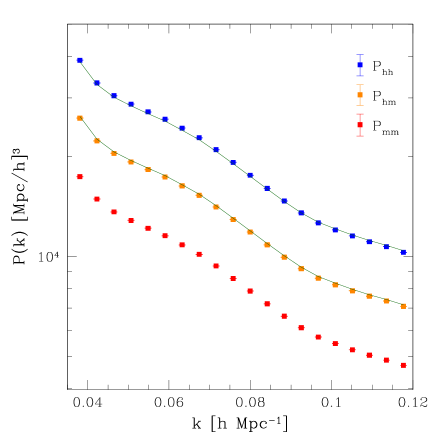
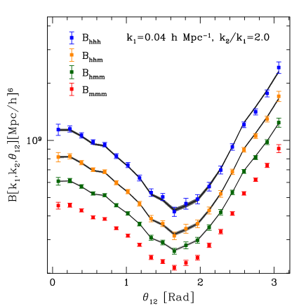
Figure 1: Power-spectra and bispectra measurements averaged over 200 ΛΛ\LambdaCDM N𝑁N-body simulations at redshift z=0𝑧0z=0. Left: Power spectra as a function of wavenumber. The blue, orange, and red symbols denote Phh,Phmsubscript𝑃hhsubscript𝑃hmP_{\rm hh},P_{\rm hm} and Pmmsubscript𝑃mmP_{\rm mm}, respectively. Right: Bispectra as a function of triangle configuration. The blue, orange, green, and red symbols represent Bhhh,Bhhm,Bhmm,Bmmmsubscript𝐡hhhsubscript𝐡hhmsubscript𝐡hmmsubscript𝐡mmmB_{\rm hhh},B_{\rm hhm},B_{\rm hmm},B_{\rm mmm}, respectively. In both panels, the errorbars show the standard error on the mean. On the other hand, the black lines denote the posterior mean for the different statistics obtained by fitting the second-order LEB to the simulation data. The shaded grey areas (which are unnoticeably narrow for the power spectrum) indicate the predictions for the models that are located within one rms value of the posterior distribution around the mean (see Β§5.3 for more details)

4 Estimating the spectra

In this section we describe how we estimate all the halo and matter polyspectra that enter the second-order LEB from the N𝑁N-body simulations at redshift z=0𝑧0z=0.

4.1 The halo auto- and cross-power and bispectra

To begin, the halo and matter density fields are interpolated onto a cubical Cartesian mesh using the cloud-in-cell (CIC) algorithm. Throughout we use mesh sizes corresponding to Ncell=10243subscript𝑁cellsuperscript10243N_{\rm cell}=1024^{3}. We then Fourier transform these grids using the Fast Fourier Transform technique and correct each mode for the CIC assignment. The three power spectra Pmmsubscript𝑃mmP_{\rm mm}, Phmsubscript𝑃hmP_{\rm hm}, Phhsubscript𝑃hhP_{\rm hh}, and the four bispectra, Bmmmsubscript𝐡mmmB_{\rm mmm}, Bhmm(s)subscriptsuperscript𝐡shmmB^{(\rm s)}_{\rm hmm}, Bhhm(s)subscriptsuperscript𝐡shhmB^{(\rm s)}_{\rm hhm}, Bhhh(s)subscriptsuperscript𝐡shhhB^{(\rm s)}_{\rm hhh}, are then estimated using the expressions:

P^α​βd​(𝐀1)subscriptsuperscript^𝑃d𝛼𝛽subscript𝐀1\displaystyle\hat{P}^{\rm d}_{\alpha\beta}({\bf k}_{1})\!\! =\displaystyle= L3N​(ki)β€‹βˆ‘iN​(ki)δα​(𝐀i)​δβ​(βˆ’π€i),superscript𝐿3𝑁subscriptπ‘˜π‘–superscriptsubscript𝑖𝑁subscriptπ‘˜π‘–subscript𝛿𝛼subscript𝐀𝑖subscript𝛿𝛽subscript𝐀𝑖\displaystyle\!\!\frac{L^{3}}{N(k_{i})}\sum_{i}^{N(k_{i})}\delta_{\alpha}({\bf k}_{i})\delta_{\beta}(-{\bf k}_{i})\;, (27)
B^α​β​γd​(𝐀1,𝐀2,ΞΈ12)subscriptsuperscript^𝐡d𝛼𝛽𝛾subscript𝐀1subscript𝐀2subscriptπœƒ12\displaystyle\hat{B}^{\rm d}_{\alpha\beta\gamma}({\bf k}_{1},{\bf k}_{2},\theta_{12})\!\! =\displaystyle= 13L6Ntriβˆ‘Ο΅β€‹(𝐀i,𝐀j)Ntriδα(𝐀i)δβ(𝐀j)Γ—\displaystyle\!\!\frac{1}{3}\frac{L^{6}}{N_{\rm tri}}\sum^{N_{\rm tri}}_{\epsilon({\bf k}_{i},{\bf k}_{j})}\delta_{\alpha}({\bf k}_{i})\delta_{\beta}({\bf k}_{j})\times (28)
×δγ​(βˆ’π€iβˆ’π€j)+2​cyc,absentsubscript𝛿𝛾subscript𝐀𝑖subscript𝐀𝑗2cyc\displaystyle\times\,\delta_{\gamma}(-{\bf k}_{i}-{\bf k}_{j})+2\,{\rm cyc}\;,

where N​(ki)𝑁subscriptπ‘˜π‘–N(k_{i}) is the number of Fourier modes in a narrow shell centred on k1subscriptπ‘˜1k_{1}, ϡ​(𝐀i,𝐀j)italic-Ο΅subscript𝐀𝑖subscript𝐀𝑗\epsilon({\bf k}_{i},{\bf k}_{j}) represents the pair of vectors which lie in thin shells centred on k1subscriptπ‘˜1k_{1} and k2subscriptπ‘˜2k_{2}, whose angular separation lies in the angular bin centred on ΞΈ12subscriptπœƒ12\theta_{12}, and Ntri≑Ntri​(ki,kj,ΞΈi​j)subscript𝑁trisubscript𝑁trisubscriptπ‘˜π‘–subscriptπ‘˜π‘—subscriptπœƒπ‘–π‘—N_{\rm tri}\equiv N_{\rm tri}(k_{i},k_{j},\theta_{ij}) is the total number of triangles with this configuration in Fourier space. The superscript β€œd” denotes that these are spectra of a discrete distribution of points (i.e. haloes) and must be corrected for shot noise. The forms of the Poissonian shot-noise corrections we adopt were presented in Pollack, Smith & Porciani (2012):

P^α​βshot​(𝐀1)subscriptsuperscript^𝑃shot𝛼𝛽subscript𝐀1\displaystyle\hat{P}^{\rm shot}_{\alpha\beta}({\bf k}_{1})\!\! =\displaystyle= δα​βKnΒ―Ξ±subscriptsuperscript𝛿K𝛼𝛽subscript¯𝑛𝛼\displaystyle\!\!\frac{\delta^{\rm K}_{\alpha\beta}}{\bar{n}_{\alpha}} (29)
B^α​β​γshot​(𝐀1,𝐀2)subscriptsuperscript^𝐡shot𝛼𝛽𝛾subscript𝐀1subscript𝐀2\displaystyle\hat{B}^{\rm shot}_{\alpha\beta\gamma}({\bf k}_{1},{\bf k}_{2})\!\! =\displaystyle= 13​δα​βKn¯α​[Pβ​γ​(𝐀1)+2​cyc]13subscriptsuperscript𝛿K𝛼𝛽subscript¯𝑛𝛼delimited-[]subscript𝑃𝛽𝛾subscript𝐀12cyc\displaystyle\frac{1}{3}\frac{\delta^{\rm K}_{\alpha\beta}}{\bar{n}_{\alpha}}\left[P_{\beta\gamma}({\bf k}_{1})+2\,{\rm cyc}\right] (30)
+13​δβ​γKn¯β​[Pγ​α​(𝐀1)+2​cyc]13subscriptsuperscript𝛿K𝛽𝛾subscript¯𝑛𝛽delimited-[]subscript𝑃𝛾𝛼subscript𝐀12cyc\displaystyle+\frac{1}{3}\frac{\delta^{\rm K}_{\beta\gamma}}{\bar{n}_{\beta}}\left[P_{\gamma\alpha}({\bf k}_{1})+2\,{\rm cyc}\right]
+13​δγ​αKn¯γ​[Pα​β​(𝐀1)+2​cyc]+δα​βK​δα​γKnΒ―Ξ±213subscriptsuperscript𝛿K𝛾𝛼subscript¯𝑛𝛾delimited-[]subscript𝑃𝛼𝛽subscript𝐀12cycsubscriptsuperscript𝛿K𝛼𝛽subscriptsuperscript𝛿K𝛼𝛾superscriptsubscript¯𝑛𝛼2\displaystyle+\frac{1}{3}\frac{\delta^{\rm K}_{\gamma\alpha}}{\bar{n}_{\gamma}}\left[P_{\alpha\beta}({\bf k}_{1})+2\,{\rm cyc}\right]+\frac{\delta^{\rm K}_{\alpha\beta}\delta^{\rm K}_{\alpha\gamma}}{\bar{n}_{\alpha}^{2}}

where nΒ―Ξ±subscript¯𝑛𝛼\bar{n}_{\alpha} denotes the mean number density of either the matter particles or the halo population.

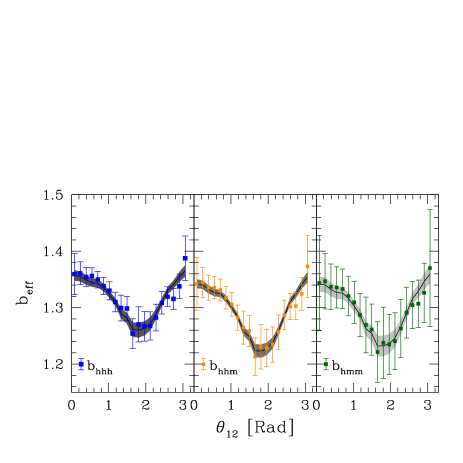
FigureΒ 1 presents the various power- and bi-spectra averaged over the 200 realizations with the corresponding standard errors on the mean. All spectra were corrected for shot noise using Eqs (29) andΒ (30). The bispectra were measured for triangle configurations with fixed lengths k1=0.04​h​Mpcβˆ’1subscriptπ‘˜10.04β„ŽsuperscriptMpc1k_{1}=0.04\,h\,{\rm Mpc}^{-1} and k2=2​k1subscriptπ‘˜22subscriptπ‘˜1k_{2}=2k_{1}, but with varying angle ΞΈ12subscriptπœƒ12\theta_{12}. We adopt the convention ΞΈ12=0subscriptπœƒ120\theta_{12}=0 for 𝐀1subscript𝐀1{\bf k}_{1} and 𝐀2subscript𝐀2{\bf k}_{2} parallel. In order to use the same range of wavenumbers, the power spectra were measured over the scale range 0.04<k<0.120.04π‘˜0.120.04<k<0.12 h​Mpcβˆ’1β„ŽsuperscriptMpc1\,h\,{\rm Mpc}^{-1}.

Refer to caption
Refer to caption
Refer to caption
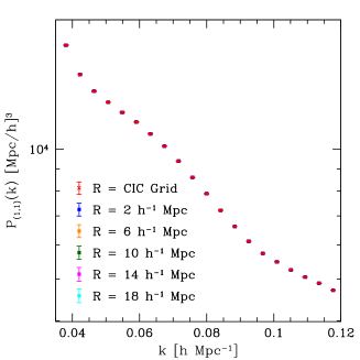
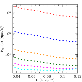
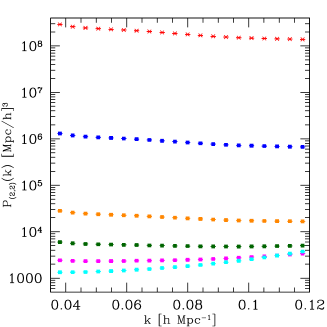
Figure 2: Measurements of the de-smoothed terms P(1,1)subscript𝑃11P_{(1,1)}, P(2,1)subscript𝑃21P_{(2,1)}, and P(2,2)subscript𝑃22P_{(2,2)} averaged over 200 N𝑁N-body simulations. We show results for a number of smoothing scales within the range 2≀R≀18​hβˆ’1​Mpc2𝑅18superscriptβ„Ž1Mpc2\leq R\leq 18\,h^{-1}{\rm Mpc} in comparison with our basic CIC grid (see the main text for more details). The errorbars denote the standard error on the mean.

4.2 Estimating P(l,m)subscriptπ‘ƒπ‘™π‘šP_{(l,m)} and B(l,m,n)(s)subscriptsuperscript𝐡sπ‘™π‘šπ‘›B^{(\rm s)}_{(l,m,n)}

The polyspectra P(l,m)subscriptπ‘ƒπ‘™π‘šP_{(l,m)} and B(l,m,n)(s)subscriptsuperscript𝐡sπ‘™π‘šπ‘›B^{(\rm s)}_{(l,m,n)} that enter the expressions for the halo power- and bi-spectra in the LEB are affected by the non-linear evolution of the matter fluctuations. While these terms are usually approximated with perturbative techniques, we measure them directly from our N𝑁N-body simulations. We do this as follows. First, we correct each Fourier mode of the mass-density field for convolution with the CIC grid. Then we multiply the result by a Gaussian smoothing function W​(k​R)=exp⁑[βˆ’(k​R)2/2]π‘Šπ‘˜π‘…superscriptπ‘˜π‘…22W(kR)=\exp\left[-(kR)^{2}/2\right] and inverse transform back to real space. Next, we generate the fields Ξ΄l​(𝐱|R)superscript𝛿𝑙conditional𝐱𝑅\delta^{l}({\bf x}|R) for the relevant values of l𝑙l and re-transform them into Fourier space. We then deconvolve these fields for the original smoothing, which means simply multiplying each Fourier mode by Wβˆ’1​(k​R)superscriptπ‘Š1π‘˜π‘…W^{-1}(kR). Finally, the required P(l,m)subscriptπ‘ƒπ‘™π‘šP_{(l,m)} and B(l,m,n)(s)subscriptsuperscript𝐡sπ‘™π‘šπ‘›B^{(\rm s)}_{(l,m,n)} terms, defined in terms of Ξ”(l)​(𝐀|R)superscriptΔ𝑙conditional𝐀𝑅\Delta^{(l)}({\bf k}|R) (see Eq. (5)), can be estimated as follows

P^(l,m)​(𝐀1)=L3N​(ki)β€‹βˆ‘iN​(ki)Ξ”(l)​(𝐀i|R)​Δ(m)​(βˆ’π€i|R),subscript^π‘ƒπ‘™π‘šsubscript𝐀1superscript𝐿3𝑁subscriptπ‘˜π‘–superscriptsubscript𝑖𝑁subscriptπ‘˜π‘–superscriptΔ𝑙conditionalsubscript𝐀𝑖𝑅superscriptΞ”π‘šconditionalsubscript𝐀𝑖𝑅\hat{P}_{(l,m)}({\bf k}_{1})=\frac{L^{3}}{N(k_{i})}\sum_{i}^{N(k_{i})}\Delta^{(l)}({\bf k}_{i}|R)\Delta^{(m)}(-{\bf k}_{i}|R)\;, (31)

and

B^(l,m,n)(s)​(𝐀1,𝐀2,ΞΈ12)subscriptsuperscript^𝐡sπ‘™π‘šπ‘›subscript𝐀1subscript𝐀2subscriptπœƒ12\displaystyle\hat{B}^{(\rm s)}_{(l,m,n)}({\bf k}_{1},{\bf k}_{2},\theta_{12}) =13L6Ntriβˆ‘Ο΅β€‹(𝐀i,𝐀j)NtriΞ”(l)(𝐀i|R)Γ—\displaystyle\!\!\!\!=\frac{1}{3}\frac{L^{6}}{N_{\rm tri}}\sum^{N_{\rm tri}}_{\epsilon({\bf k}_{i},{\bf k}_{j})}\Delta^{(l)}({\bf k}_{i}|R)\times (32)
Γ—Ξ”(m)​(𝐀j|R)​Δ(n)​(βˆ’π€iβˆ’π€j|R)+2​cyc.absentsuperscriptΞ”π‘šconditionalsubscript𝐀𝑗𝑅superscriptΔ𝑛subscript𝐀𝑖conditionalsubscript𝐀𝑗𝑅2cyc\displaystyle\!\!\!\!\!\!\!\!\!\!\!\!\!\!\!\!\!\!\!\!\!\!\!\!\!\!\!\!\!\!\!\!\times\,\Delta^{(m)}({\bf k}_{j}|R)\Delta^{(n)}(-{\bf k}_{i}-{\bf k}_{j}|R)+2\,{\rm cyc}\;.
Refer to caption
Refer to caption
Refer to caption
Refer to caption
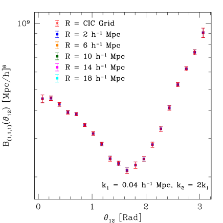
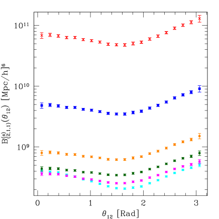
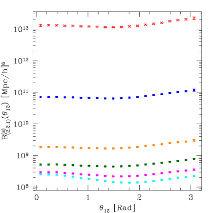
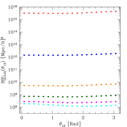
Figure 3: Same as for Figure 2 but for the bispectrum terms B(1,1,1)subscript𝐡111B_{(1,1,1)}, B(2,1,1)(s)subscriptsuperscript𝐡s211B^{(\rm s)}_{(2,1,1)}, B(2,2,1)(s)subscriptsuperscript𝐡s221B^{(\rm s)}_{(2,2,1)}, and B(2,2,2)(s)subscriptsuperscript𝐡s222B^{(\rm s)}_{(2,2,2)}.

We note that the functions P(l,m)subscriptπ‘ƒπ‘™π‘šP_{(l,m)} and B(l,m,n)(s)subscriptsuperscript𝐡sπ‘™π‘šπ‘›B^{(\rm s)}_{(l,m,n)} slowly vary with R𝑅R and so can be smoothly interpolated. Based on this knowledge, we measure the spectral functions over the range: R=[2, 18]​hβˆ’1​Mpc𝑅218superscriptβ„Ž1MpcR=\left[2,\,18\right]\,h^{-1}{\rm Mpc}, in increments of △​R=2△𝑅2\triangle R=2 hβˆ’1​Mpcsuperscriptβ„Ž1Mpc\,h^{-1}{\rm Mpc}, but including an additional measurement at R=7𝑅7R=7 hβˆ’1​Mpcsuperscriptβ„Ž1Mpc\,h^{-1}{\rm Mpc}. The lower limit was adopted because we do not wish to smooth below the Lagrangian size of haloes, which for our sample is of the order of ∼3βˆ’4​hβˆ’1​Mpcsimilar-toabsent34superscriptβ„Ž1Mpc\sim 3-4\,\,h^{-1}{\rm Mpc}. The upper bound of R=18​hβˆ’1​Mpc𝑅18superscriptβ„Ž1MpcR=18\,h^{-1}{\rm Mpc} we justify by noting that we do not want the largest kπ‘˜k-mode entering our computations of the halo power- and bi-spectra to be too heavily smoothed.

Before inspecting the functions P(l,m)subscriptπ‘ƒπ‘™π‘šP_{(l,m)} and B(l,m,n)(s)subscriptsuperscript𝐡sπ‘™π‘šπ‘›B^{(\rm s)}_{(l,m,n)}, we first report the level of non-linearity present in the smoothed matter-density field, δ​(𝐱|R)𝛿conditional𝐱𝑅\delta({\bf x}|R). We quantify this by measuring the variance of the density perturbations, Οƒ2​(R)superscript𝜎2𝑅\sigma^{2}(R) and the fraction of cells where the density contrast exceeds unity, f𝑓f, as a function of the filter scale (see Table 1). Our results show that Οƒ2​(R)<1superscript𝜎2𝑅1\sigma^{2}(R)<1 for R≳4​hβˆ’1​Mpcgreater-than-or-equivalent-to𝑅4superscriptβ„Ž1MpcR\gtrsim 4\,h^{-1}{\rm Mpc}. We therefore expect the quadratic bias model to be a poor description for smaller values of R𝑅R. However, we note that the fraction of the cells with Ξ΄β‰₯1𝛿1\delta\geq 1 is f≲0.1less-than-or-similar-to𝑓0.1f\lesssim 0.1 for all of the filter scales considered. Furthermore, in our previous work (Pollack, Smith & Porciani, 2012), we evaluated the scatter plots of Ξ΄hsubscriptπ›Ώβ„Ž\delta_{h} versus δ𝛿\delta measured from our N𝑁N-body simulations for different smoothing radii. We found that expressing Ξ΄hsubscript𝛿h\delta_{\rm h} as a polynomial function at second-order in δ𝛿\delta can describe reasonably well the mean trend of the scatter.

Table 1: Level of non-linearity in the smoothed mass-density field at redhift z=0𝑧0z=0. Column 1: filter scale, R𝑅R; Column 2: variance of density fluctuations, Οƒ2​(R)superscript𝜎2𝑅\sigma^{2}(R); Column 3: volume fraction with |δ​(R)|>1𝛿𝑅1|\delta(R)|>1, f𝑓f.
R​[hβˆ’1​Mpc]𝑅delimited-[]superscriptβ„Ž1MpcR\,[\,h^{-1}{\rm Mpc}] Οƒ2​(R)superscript𝜎2𝑅\sigma^{2}(R) 100Γ—f100𝑓100\times f
2 2.44 10.0
4 0.71 8.4
6 0.38 6.0
7 0.28 4.9
8 0.22 3.8
10 0.15 2.2
12 0.10 1.1
14 0.08 0.5
16 0.06 0.2
18 0.05 0.1
Refer to caption
Refer to caption
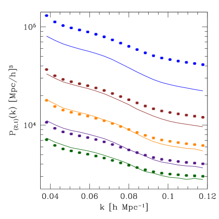
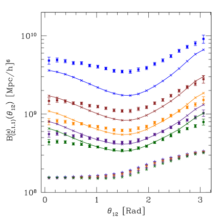
Figure 4: Left: Measurements of the P(2,1)subscript𝑃21P_{(2,1)} term from the simulations (points with errorbars) are compared with the analytical predictions from leading-order SPT (solid lines) for different filter radii (from top to bottom: R=2,4,6,8,10​hβˆ’1​Mpc𝑅246810superscriptβ„Ž1MpcR=2,4,6,8,10\,h^{-1}{\rm Mpc}). Right: Same as in the left panel but for B(2,1,1)(s)subscriptsuperscript𝐡s211B^{(\rm s)}_{(2,1,1)}. The star-shaped points represent the contribution to B(2,1,1)(s)subscriptsuperscript𝐡s211B^{(\rm s)}_{(2,1,1)} from the disconnected parts of the fourth-order correlators at tree level in SPT (i.e. cyclical products of the linear power spectrum).

4.3 Results for P(l,m)subscriptπ‘ƒπ‘™π‘šP_{(l,m)} and B(l,m,n)subscriptπ΅π‘™π‘šπ‘›B_{(l,m,n)}

FiguresΒ 2 and Β 3 show the results for the ensemble-averaged de-smoothed power and bispectra, P(l,m)subscriptπ‘ƒπ‘™π‘šP_{(l,m)} and B(l,m,n)subscriptπ΅π‘™π‘šπ‘›B_{(l,m,n)}, respectively. Focusing on the power spectrum, the panels show (from left to right) the matter power spectrum P=P(1,1)=Pmm𝑃subscript𝑃11subscript𝑃mmP=P_{(1,1)}=P_{\rm mm} followed by the terms P(2,1)subscript𝑃21P_{(2,1)}, and P(2,2)subscript𝑃22P_{(2,2)}.

For the bispectra, the panels show: the matter bispectrum B=B(1,1,1)=Bmmm𝐡subscript𝐡111subscript𝐡mmmB=B_{(1,1,1)}=B_{\rm mmm} (top left), B(2,1,1)(s)superscriptsubscript𝐡211sB_{(2,1,1)}^{\rm(s)} (top right), B(2,2,1)(s)superscriptsubscript𝐡221sB_{(2,2,1)}^{\rm(s)} (bottom left), and B(2,2,2)(s)superscriptsubscript𝐡222sB_{(2,2,2)}^{\rm(s)} (bottom right). We have restricted the triangle configurations to those which enter the auto- and cross- halo bispectra shown in Figure 1. Each panel shows six sets of points with errorbars which denote the results obtained for different smoothing scales. The red crosses denote the resulting polyspectra when no Gaussian smoothing (and de-smoothing) is applied on top of the CIC assignment.

Comparing the different panels reveals how the amplitudes of the de-smoothed quantities vary. Obviously, for the matter power and bispectra, P(1,1)subscript𝑃11P_{(1,1)} and B(1,1,1)subscript𝐡111B_{(1,1,1)}, all of the spectra overlap with the CIC result as the smoothing and the de-smoothing procedures perfectly cancel each other out. However, for the remaining P(l,m)subscriptπ‘ƒπ‘™π‘šP_{(l,m)} and B(l,m,n)subscriptπ΅π‘™π‘šπ‘›B_{(l,m,n)} functions, the de-smoothed quantities vary with the scale R𝑅R. In particular, as R𝑅R decreases, the overall amplitude of the spectra increases due to the contributions of small-scale modes. For the largest smoothing scales, the configuration dependence of the spectra is also modified. In order to gain some insight into the origin of this behaviour, let us consider, for instance, the term

P(2,1)​(𝐀)=∫d3​πͺ(2​π)3​B​(πͺ,π€βˆ’πͺ,βˆ’π€)​𝒲​(πͺ,π€βˆ’πͺ)subscript𝑃21𝐀superscriptd3πͺsuperscript2πœ‹3𝐡πͺ𝐀πͺ𝐀𝒲πͺ𝐀πͺP_{(2,1)}({\bf k})=\int\frac{{\rm d}^{3}{\bf q}}{(2\pi)^{3}}\,B({\bf q},{\bf k}-{\bf q},-{\bf k})\,\mathcal{W}({\bf q},{\bf k}-{\bf q}) (33)

where 𝒲𝒲\mathcal{W} is a generic weighting function defined as

𝒲​(𝐀1,𝐀2)=W​(k1​R)​W​(k2​R)W​(|𝐀1+𝐀2|​R).𝒲subscript𝐀1subscript𝐀2π‘Šsubscriptπ‘˜1π‘…π‘Šsubscriptπ‘˜2π‘…π‘Šsubscript𝐀1subscript𝐀2𝑅\mathcal{W}({\bf k}_{1},{\bf k}_{2})=\frac{W(k_{1}R)\,W(k_{2}R)}{W(|{\bf k}_{1}+{\bf k}_{2}|R)}\,. (34)

For Gaussian smoothing, the weighting function in Eq. (33) can be re-expressed as 𝒲​(πͺ,π€βˆ’πͺ)=exp⁑[βˆ’R2​(q2βˆ’k​q​μ)]𝒲πͺ𝐀πͺsuperscript𝑅2superscriptπ‘ž2π‘˜π‘žπœ‡\mathcal{W}({\bf q},{\bf k}-{\bf q})=\exp{\left[-R^{2}\left(q^{2}-kq\mu\right)\right]}, with ΞΌ=𝐀⋅πͺ/(k​q)πœ‡β‹…π€πͺπ‘˜π‘ž\mu={\bf k}\cdot{\bf q}/(kq) the cosine of the angle between 𝐀𝐀{\bf k} and πͺπͺ{\bf q}. The contribution to the integral from all modes with q​R≫1much-greater-thanπ‘žπ‘…1qR\gg 1 is exponentially suppressed (i.e. 𝒲β‰ͺ1much-less-than𝒲1\mathcal{W}\ll 1).

The contribution to the integral from all modes with q​R≫1much-greater-thanπ‘žπ‘…1qR\gg 1 is exponentially suppressed (i.e. 𝒲β‰ͺ1much-less-than𝒲1\mathcal{W}\ll 1). However, at fixed kπ‘˜k, 𝒲𝒲\mathcal{W} assumes values larger than unity for ΞΌ>0πœ‡0\mu>0 and q<kβ€‹ΞΌπ‘žπ‘˜πœ‡q<k\mu (independently of R𝑅R) and presents an absolute maximum for q=k/2π‘žπ‘˜2q=k/2 and ΞΌ=1πœ‡1\mu=1 where it takes the value 𝒲max=exp⁑[(k​R)2/4]subscript𝒲maxsuperscriptπ‘˜π‘…24\mathcal{W}_{\rm max}=\exp[(kR)^{2}/4]. Note that, when k​Rβ‰ͺ1much-less-thanπ‘˜π‘…1kR\ll 1, 𝒲max≃1+(k​R)2/4≃1similar-to-or-equalssubscript𝒲max1superscriptπ‘˜π‘…24similar-to-or-equals1\mathcal{W}_{\rm max}\simeq 1+(kR)^{2}/4\simeq 1 so that all configurations where 𝒲>1𝒲1\mathcal{W}>1 receive nearly the same weight. In this case, the parameter R𝑅R regulates how quickly the function 𝒲𝒲\mathcal{W} drops when qπ‘žq moves away from the region where 𝒲>1𝒲1\mathcal{W}>1. In other words, 𝒲𝒲\mathcal{W} behaves nicely as a smoothing function. This is not true, however, when k​R≫1much-greater-thanπ‘˜π‘…1kR\gg 1 and the value of 𝒲maxsubscript𝒲max\mathcal{W}_{\rm max} grows very large. In this case, P(2,1)subscript𝑃21P_{(2,1)} receives dominant contributions from a narrow shell of modes located at q≃k/2similar-to-or-equalsπ‘žπ‘˜2q\simeq k/2 and μ≲1less-than-or-similar-toπœ‡1\mu\lesssim 1. This effect is clearly seen in FigureΒ 2 for R=18𝑅18R=18 hβˆ’1​Mpcsuperscriptβ„Ž1Mpc\,h^{-1}{\rm Mpc} where the over-smoothing (i.e. the fact that k​Rπ‘˜π‘…kR is significantly larger than unity for k∼0.1similar-toπ‘˜0.1k\sim 0.1) leads to a change in shape for P(2,1)subscript𝑃21P_{(2,1)} which is particularly evident for the configurations with the largest wavenumbers.

It is interesting to investigate why, for k​Rβ‰ͺ1much-less-thanπ‘˜π‘…1kR\ll 1, the configuration dependence of P(2,1)subscript𝑃21P_{(2,1)} changes very little with R𝑅R and only the overall normalisation appears to depend on the smoothing scale. If we assume that the amplitude of the bispectrum B​(𝐀1,𝐀2,βˆ’π€1βˆ’π€2)𝐡subscript𝐀1subscript𝐀2subscript𝐀1subscript𝐀2B({\bf k}_{1},{\bf k}_{2},-{\bf k}_{1}-{\bf k}_{2}) keeps nearly constant at all scales assuming a value ≃B0similar-to-or-equalsabsentsubscript𝐡0\simeq B_{0}, Equation (33) then gives

P(2,1)​(𝐀)≃π3/2​exp⁑((k​R)2/4)R3​B0.similar-to-or-equalssubscript𝑃21𝐀superscriptπœ‹32superscriptπ‘˜π‘…24superscript𝑅3subscript𝐡0P_{(2,1)}({\bf k})\simeq\frac{\pi^{3/2}\exp{((kR)^{2}/4)}}{R^{3}}\,B_{0}\;. (35)

The first term on the right-hand-side gives the qπ‘žq-space volume over which the bispectrum is averaged to get P(2,1)subscript𝑃21P_{(2,1)}. At fixed kπ‘˜k, this expression diverges as Rβˆ’3superscript𝑅3R^{-3} when Rβ†’0→𝑅0R\to 0 and exponentially as Rβ†’βˆžβ†’π‘…R\to\infty while it shows broad minimum around k​R∼2.5similar-toπ‘˜π‘…2.5kR\sim 2.5.

Clearly, had we not smoothed the density field, the resulting P(l,m)subscriptπ‘ƒπ‘™π‘šP_{(l,m)} and B(l,m,n)subscriptπ΅π‘™π‘šπ‘›B_{(l,m,n)} would be divergent in any ΛΛ\LambdaCDM cosmology.

4.4 Modelling P(2,1)subscript𝑃21P_{(2,1)} and B(2,1,1)(s)subscriptsuperscript𝐡s211B^{\rm(s)}_{(2,1,1)} with SPT

In order to better understand what drives the amplitude and functional form of the P(l,m)subscriptπ‘ƒπ‘™π‘šP_{(l,m)} and B(l,m,n)(s)subscriptsuperscript𝐡sπ‘™π‘šπ‘›B^{\rm(s)}_{(l,m,n)} terms we have attempted to model their signal with SPT. For simplicity, we have focused on the lowest-order non-trivial terms P(2,1)subscript𝑃21P_{(2,1)} and B(2,1,1)(s)subscriptsuperscript𝐡s211B^{\rm(s)}_{(2,1,1)}.

To leading order in the perturbations, the matter bispectrum can be written as B​(𝐀1,𝐀2,𝐀3)=2​F2​(𝐀1,𝐀2)​P(0)​(k1)​P(0)​(k2)+2​cyc𝐡subscript𝐀1subscript𝐀2subscript𝐀32subscript𝐹2subscript𝐀1subscript𝐀2subscript𝑃0subscriptπ‘˜1subscript𝑃0subscriptπ‘˜22cycB({\bf k}_{1},{\bf k}_{2},{\bf k}_{3})=2\,F_{2}({\bf k}_{1},{\bf k}_{2})\,P_{(0)}(k_{1})\,P_{(0)}(k_{2})+{\rm 2\ cyc} with F2subscript𝐹2F_{2} the second-order SPT kernel (see Appendix B) and P(0)subscript𝑃0P_{(0)} the linear power spectrum. In Figure 4 (left panel) we show the results obtained after inserting this expression into Equation (33) in comparison with the P(2,1)subscript𝑃21P_{(2,1)} measurements from the N𝑁N-body simulations. The SPT-based model displays the same scaling behaviour with kπ‘˜k and R𝑅R as the data. However, for R>6​hβˆ’1​Mpc𝑅6superscriptβ„Ž1MpcR>6\,h^{-1}{\rm Mpc} the SPT predictions are accurate to better than 131313 per cent, which is still not at the level of precision required for future galaxy clustering datasets; the deviations become larger with smaller R𝑅R. It follows from the definition of the B(2,1,1)(s)subscriptsuperscript𝐡s211B^{\rm(s)}_{(2,1,1)} term that (see Appendix B for ℬ(2,1,1)(s)subscriptsuperscriptℬs211\mathcal{B}^{\rm(s)}_{(2,1,1)})

B(2,1,1)(s)subscriptsuperscript𝐡s211\displaystyle B^{\rm(s)}_{(2,1,1)}\!\!\!\!\!\! (𝐀1,𝐀2,𝐀3)=23​[P​(𝐀2)​P​(𝐀3)​𝒲​(𝐀2,𝐀3)+2​cyc]+subscript𝐀1subscript𝐀2subscript𝐀3limit-from23delimited-[]𝑃subscript𝐀2𝑃subscript𝐀3𝒲subscript𝐀2subscript𝐀32cyc\displaystyle\!\!\!\!\!\!\!\!({\bf k}_{1},{\bf k}_{2},{\bf k}_{3})=\frac{2}{3}\left[P({\bf k}_{2})P({\bf k}_{3})\mathcal{W}({\bf k}_{2},{\bf k}_{3})+2\ {\rm cyc}\right]+ (36)
+13β€‹βˆ«d3​πͺ1(2​π)3​T​(πͺ1,𝐀1βˆ’πͺ1,𝐀2,𝐀3)​𝒲​(πͺ1,𝐀1βˆ’πͺ1)13superscriptd3subscriptπͺ1superscript2πœ‹3𝑇subscriptπͺ1subscript𝐀1subscriptπͺ1subscript𝐀2subscript𝐀3𝒲subscriptπͺ1subscript𝐀1subscriptπͺ1\displaystyle+\,\,\frac{1}{3}\int\frac{{\rm d}^{3}{\bf q}_{1}}{(2\pi)^{3}}T({\bf q}_{1},{\bf k}_{1}-{\bf q}_{1},{\bf k}_{2},{\bf k}_{3})\mathcal{W}({\bf q}_{1},{\bf k}_{1}-{\bf q}_{1})
+  2​cyc,2cyc\displaystyle+\,\,{2\ \rm cyc}\;,

where T𝑇T denotes the matter trispectrum (i.e. the connected part of the 444-point correlator). The SPT contribution to lowest non-vanishing order is simply:

B(2,1,1)(s)​(𝐀1,𝐀2,𝐀3)≃23​[P(0)​(𝐀2)​P(0)​(𝐀3)​𝒲​(𝐀2,𝐀3)+2​cyc].similar-to-or-equalssubscriptsuperscript𝐡s211subscript𝐀1subscript𝐀2subscript𝐀323delimited-[]subscript𝑃0subscript𝐀2subscript𝑃0subscript𝐀3𝒲subscript𝐀2subscript𝐀32cycB^{\rm(s)}_{(2,1,1)}({\bf k}_{1},{\bf k}_{2},{\bf k}_{3})\simeq\frac{2}{3}\!\left[P_{(0)}({\bf k}_{2})P_{(0)}({\bf k}_{3})\mathcal{W}({\bf k}_{2},{\bf k}_{3})+2\ {\rm cyc}\right]\;\!. (37)

In the right panel of FigureΒ 4 we show that this approximation (star-shaped points) strongly underestimates the outcome from the N𝑁N-body simulations (solid symbols with errorbars) and does not display the same scaling behaviour with kπ‘˜k and R𝑅R as the data. A common approach performed during observational data analysis is to substitute in place of the linear power spectrum, P(0)subscript𝑃0P_{(0)}, shown in Eq. 37, the fully non-linear power spectrum, P(1,1)subscript𝑃11P_{(1,1)}. We found that performing this substitution has little effect on the resulting amplitudes, remaining roughly equivalent as the lowest nonvanishing contributions. We then go one step further and compute the next-to-leading-order corrections to B(2,1,1)(s)subscriptsuperscript𝐡s211B^{\rm(s)}_{(2,1,1)} which are of sixth-order in terms of the linear density field. This gives

B(2,1,1)(s)subscriptsuperscript𝐡s211\displaystyle B^{\rm(s)}_{(2,1,1)}\!\!\!\!\!\!\!\! (𝐀1,𝐀2,𝐀3)≃23𝒲(𝐀2,𝐀3)[P(0)(𝐀2)P(0)(𝐀3)+\displaystyle\!\!\!\!\!\!\!\!({\bf k}_{1},{\bf k}_{2},{\bf k}_{3})\simeq\frac{2}{3}\mathcal{W}({\bf k}_{2},{\bf k}_{3})\left[\frac{}{}P_{(0)}({\bf k}_{2})P_{(0)}({\bf k}_{3})+\right. (38)
+\displaystyle+ P(0)(𝐀2)P(1​ℓ)(𝐀3)+P(1​ℓ)(𝐀2)P(0)(𝐀3)]+2cyc\displaystyle\!\!\!\!\!\left.P_{(0)}({\bf k}_{2})P_{(1\ell)}({\bf k}_{3})\right.+\!\!\left.\frac{}{}P_{(1\ell)}({\bf k}_{2})P_{(0)}({\bf k}_{3})\right]+2\ {\rm cyc}
+13β€‹βˆ«d3​πͺ1(2​π)3​𝒲​(πͺ1,𝐀1βˆ’πͺ1)​T(0)​(πͺ1,𝐀1βˆ’πͺ1,𝐀2,𝐀3)13superscriptd3subscriptπͺ1superscript2πœ‹3𝒲subscriptπͺ1subscript𝐀1subscriptπͺ1subscript𝑇0subscriptπͺ1subscript𝐀1subscriptπͺ1subscript𝐀2subscript𝐀3\displaystyle\!\!\!\!\!\!\!\!\!\!\!+\,\,\frac{1}{3}\int\frac{{\rm d}^{3}{\bf q}_{1}}{(2\pi)^{3}}\mathcal{W}({\bf q}_{1},{\bf k}_{1}-{\bf q}_{1})T_{(0)}({\bf q}_{1},{\bf k}_{1}-{\bf q}_{1},{\bf k}_{2},{\bf k}_{3})
+  2​cyc,2cyc\displaystyle\!\!\!\!\!\!\!\!\!\!\!+\,\,{2\ \rm cyc}\ ,

where P(1​ℓ)subscript𝑃1β„“P_{(1\ell)} denotes the first loop correction to the power spectrum (i.e. P≃P(0)+P(1​ℓ)+…similar-to-or-equals𝑃subscript𝑃0subscript𝑃1ℓ…P\simeq P_{(0)}+P_{(1\ell)}+\dots) and the term T0subscript𝑇0T_{\rm 0} represents the tree-level contribution to the connected trispectrum. In AppendixΒ B we provide the expressions needed for evaluating all these quantities, which are de-smoothed according to Eq. (15). Our final results are shown in FigureΒ 4 (solid lines). The SPT approximation shows the correct scaling with R𝑅R, but for R>2​hβˆ’1​Mpc𝑅2superscriptβ„Ž1MpcR>2\,h^{-1}{\rm Mpc} it tends to overpredict the amplitude for collinear (i.e. θ≃0similar-to-or-equalsπœƒ0\theta\simeq 0 and θ≃πsimilar-to-or-equalsπœƒπœ‹\theta\simeq\pi) configurations. For 4<R≀8​hβˆ’1​Mpc4𝑅8superscriptβ„Ž1Mpc4<R\leq 8\,h^{-1}{\rm Mpc} it also underpredicts the amplitude for triangles in which 𝐀1subscript𝐀1{\bf k}_{1} and 𝐀2subscript𝐀2{\bf k}_{2} are nearly perpendicular. However, as R𝑅R increases the discrepancy lessens and at R=10​hβˆ’1​Mpc𝑅10superscriptβ„Ž1MpcR=10\,h^{-1}{\rm Mpc} SPT performs better. This suggests that using SPT to fit galaxy bispectra in the scale range 0.04≲k≲0.12​h​Mpcβˆ’1less-than-or-similar-to0.04π‘˜less-than-or-similar-to0.12β„ŽsuperscriptMpc10.04\lesssim k\lesssim 0.12\,h\,{\rm Mpc}^{-1} may possibly lead to seriously biased estimates for the parameters of the LEB.

Nevertheless, whilst the analytic calculations of 𝒫(2,1)subscript𝒫21{\mathcal{P}}_{(2,1)} and ℬ(2,1,1)(s)subscriptsuperscriptℬs211{\mathcal{B}}^{\rm(s)}_{(2,1,1)} are feasible, computing higher-order terms becomes increasingly challenging. However, estimating these quantities from simulations is no more demanding than measuring the low-order terms and so our approach offers a distinct advantage over the classical SPT calculations.

5 Estimation of halo bias

5.1 Bayesian parameter estimation

The second-order LEB contains three parameters: πœ½β‰‘{b1,b2,R}𝜽subscript𝑏1subscript𝑏2𝑅\bm{\theta}\equiv\{b_{1},b_{2},R\}. In this section, we use Bayesian statistics to determine their values that best represent the halo power and bispectra extracted from our simulations. For simplicity, we assume that the cosmological parameters are perfectly known and that the measurement errors are Gaussian distributed, i.e.

ℒ​(𝐱|𝜽)β„’conditional𝐱𝜽\displaystyle{\mathcal{L}}({\bf x}|\bm{\theta})\!\!\!\!\! =\displaystyle= (2​π)βˆ’N/2​|C|βˆ’1/2​eβˆ’12​[(π±βˆ’ΞΌβ€‹(𝜽))T​Cβˆ’1​(π±βˆ’ΞΌβ€‹(𝜽))]=superscript2πœ‹π‘2superscriptC12superscripte12delimited-[]superscriptπ±πœ‡πœ½TsuperscriptC1π±πœ‡πœ½absent\displaystyle\!\!\!\!\!(2\pi)^{-N/2}\,|{\textbf{{C}}}|^{-1/2}{\rm e}^{-\frac{1}{2}[({\bf x}-\mu(\bm{\theta}))^{\rm T}\textbf{{C}}^{-1}({\bf x}-\mu(\bm{\theta}))]}\;=
=\displaystyle= (2​π)βˆ’N/2​|C|βˆ’1/2​eβˆ’Ο‡2​(𝐱,𝜽)2,superscript2πœ‹π‘2superscriptC12superscriptesuperscriptπœ’2𝐱𝜽2\displaystyle\!\!\!\!\!(2\pi)^{-N/2}\,|{\textbf{{C}}}|^{-1/2}{\rm e}^{-\frac{\chi^{2}({\bf x},\bm{\theta})}{2}}\;,

where 𝐱Tsuperscript𝐱T{\bf x}^{\rm T} is the N𝑁N-dimensional vector containing the power spectra or bispectra for different configurations, μ​(𝜽)πœ‡πœ½\mu(\bm{\theta}) is the model prediction and C is the covariance matrix. In theory C is a model dependent quantity, however owing to the technical challenge of estimating this matrix and its inverse, we have decided to determine C directly from the data.

Equation (5.1) gives the likelihood of the data given the model, but what we need in order to perform parameter estimation is the posterior probability of the model parameters given the data. This can be obtained using Bayes’ theorem:

P​(𝜽|𝐱)=Π​(𝜽)​ℒ​(𝐱|𝜽)p​(𝐱),𝑃conditionalπœ½π±Ξ πœ½β„’conditionalπ±πœ½π‘π±P(\bm{\theta}|{\bf x})=\frac{\Pi(\bm{\theta})\,{\mathcal{L}}({\bf x}|\bm{\theta})}{p({\bf x})}\ , (40)

where Π​(𝜽)Π𝜽\Pi(\bm{\theta}) is the prior probability for the model parameter while the evidence,

p​(𝐱)β‰‘βˆ«Ξ β€‹(𝜽)​ℒ​(𝐱|𝜽)​d3​θ,π‘π±Ξ πœ½β„’conditional𝐱𝜽superscript𝑑3πœƒp({\bf x})\equiv\int\Pi(\bm{\theta})\,{\mathcal{L}}({\bf x}|\bm{\theta})\,d^{3}\,\theta\ , (41)

simply acts as a normalizing factor and does not influence the search for the best fit. In what follows we will always assume flat priors on the parameters, but bounded over a finite domain which is much more extended than the likelihood function. Moreover, b1subscript𝑏1b_{1} and R𝑅R will always be assumed to be positive.

5.2 Covariance matrix estimation

The sample covariance matrix

S^≑NNβˆ’1β€‹βŸ¨Ξ”β€‹π±Tβ€‹Ξ”β€‹π±βŸ©N;Ξ”β€‹π±β‰‘π±βˆ’βŸ¨π±βŸ©N,formulae-sequence^S𝑁𝑁1subscriptdelimited-βŸ¨βŸ©Ξ”superscript𝐱TΔ𝐱𝑁Δ𝐱𝐱subscriptdelimited-βŸ¨βŸ©π±π‘\widehat{{\textbf{{S}}}}\equiv\frac{N}{N-1}\langle\Delta{\bf x}^{\rm T}\Delta{\bf x}\rangle_{N}\ ;\hskip 14.22636pt\Delta{\bf x}\equiv{\bf x}-\langle{\bf x}\rangle_{N}\;, (42)

where βŸ¨β€¦βŸ©Nsubscriptdelimited-βŸ¨βŸ©β€¦π‘\langle\dots\rangle_{N} denotes the arithmetic mean over N𝑁N independent measurements, provides an unbiased estimator of the covariance matrix for the measurement errors.

However, this estimator is extremely unstable and inefficient. It generally provides matrices where the smallest eigenvalue is too small and the largest one is too big. Very large samples are thus needed to obtain accurate estimates of the covariance.

On using our ensemble of 200 simulations for both the power and the bispectra, we could measure the diagonal elements of the covariance with an accuracy of ∼10similar-toabsent10\sim 10 per cent. On the other hand, the off-diagonal elements had a much smaller absolute value and were scattering around zero with errors of the order of ∼100similar-toabsent100\sim 100 per cent. All this suggests that the covariance should be close to diagonal as expected for a Gaussian random field with infinitesimally narrow bins in kπ‘˜k-space.

Due to these large uncertainties in the off-diagonal elements, we opted for implementing a shrinkage method to better estimate the covariance matrices of our power and bispectra. Shrinkage estimation is a variance reduction technique that shrinks an empirical estimation of the covariance like S^^S\widehat{{\textbf{{S}}}} towards a theoretical model for how the covariance should be, represented by a structured matrix T (the target covariance). The shrinked estimator is given by the convex linear combination

C^=λ​T+(1βˆ’Ξ»)​S^^Cπœ†T1πœ†^S\widehat{\textbf{{C}}}=\lambda{\textbf{{T}}}+(1-\lambda)\widehat{\textbf{{S}}} (43)

where 0<Ξ»<10πœ†10<\lambda<1 is the shrinkage intensity. This ensures the resulting covariance matrix to be positive definite even if S^^S\widehat{\textbf{{S}}} is singular (because it is determined from N<dim​(𝐱)𝑁dim𝐱N<{\mathrm{dim}}({\bf x}) observations).

It has been demonstrated that shrinkage techniques provide a regularized estimate of the covariance S^^S\widehat{\textbf{{S}}} which is both more accurate and statistically efficient than either of the individual estimators S^^S\widehat{\textbf{{S}}} and T, and they do so in a systematic way (SchΓ€efer & Strimmer, 2005). Without the need for specifying an underlying probability distribution, Ledoit & Wolf (2003) provided a theorem that determines the optimal value for Ξ»πœ†\lambda through minimization of a quadratic loss function such as the mean-square error of the covariance matrix. This can be expressed in terms of the squared Frobenius norm

L​(Ξ»)πΏπœ†\displaystyle L(\lambda) =\displaystyle= β€–C^βˆ’πšΊβ€–π…πŸsubscriptsuperscriptnorm^C𝚺2𝐅\displaystyle\parallel\widehat{\textbf{{C}}}-\bf{\Sigma}\parallel^{2}_{F} (44)
=\displaystyle= ‖λ​T+(1βˆ’Ξ»)​S^βˆ’πšΊβ€–π…subscriptnormπœ†T1πœ†^SπšΊπ…\displaystyle\parallel\lambda\textbf{{T}}+(1-\lambda)\widehat{\textbf{{S}}}-\bf{\Sigma}\parallel_{F}
=\displaystyle= βˆ‘i,j=1p(λ​ti​j+(1βˆ’Ξ»)​si​jβˆ’Οƒi​j)2.superscriptsubscript𝑖𝑗1𝑝superscriptπœ†subscript𝑑𝑖𝑗1πœ†subscript𝑠𝑖𝑗subscriptπœŽπ‘–π‘—2\displaystyle\sum_{i,j=1}^{p}(\lambda t_{ij}+(1-\lambda)s_{ij}-\sigma_{ij})^{2}\ .

which gives a measure of the distance between the true population covariance, 𝚺𝚺\bf{\Sigma}, and the inferred one, namely, C^^C\widehat{\textbf{{C}}}. The key is to select a suitable target, and we assume it to be a diagonal matrix with unequal variances coinciding with the sample variances:

ti​j={si​i,if i = j0,if iΒ β‰ Β j.subscript𝑑𝑖𝑗casessubscript𝑠𝑖𝑖if i = j0if iΒ β‰ Β jt_{ij}=\begin{cases}{s}_{ii},&\text{if i = j}\\ 0,&\text{if i $\neq$ j}\end{cases}\;. (45)

Minimizing Eq. (44) gives the expression for the optimal shrinkage intensity:

Ξ»βˆ—=βˆ‘j>iVar​(si​j)βˆ‘j>i[Var​(si​j)+Οƒi​j2]=βˆ‘j>iVar​(si​j)βˆ‘j>iE​(si​j2),subscriptπœ†subscript𝑗𝑖Varsubscript𝑠𝑖𝑗subscript𝑗𝑖delimited-[]Varsubscript𝑠𝑖𝑗superscriptsubscriptπœŽπ‘–π‘—2subscript𝑗𝑖Varsubscript𝑠𝑖𝑗subscript𝑗𝑖Esuperscriptsubscript𝑠𝑖𝑗2\lambda_{*}=\frac{\sum_{j>i}{\textrm{Var}}(s_{ij})}{\sum_{j>i}[\textrm{Var}(s_{ij})+\sigma_{ij}^{2}]}=\frac{\sum_{j>i}{\textrm{Var}}(s_{ij})}{\sum_{j>i}\textrm{E}(s_{ij}^{2})}\,, (46)

where E​(…)E…{\textrm{E}}(\dots) denotes the expectation value of a random variable. Following SchΓ€efer & Strimmer (2005), we estimate the sampling variance of the elements of the sample covariance using

Var^​(si​j)=N(Nβˆ’1)3β€‹βˆ‘j=1N(Δ​𝐱jT​Δ​𝐱jβˆ’βŸ¨Ξ”β€‹π±Tβ€‹Ξ”β€‹π±βŸ©N)2.^Varsubscript𝑠𝑖𝑗𝑁superscript𝑁13superscriptsubscript𝑗1𝑁superscriptΞ”superscriptsubscript𝐱𝑗TΞ”subscript𝐱𝑗subscriptdelimited-βŸ¨βŸ©Ξ”superscript𝐱TΔ𝐱𝑁2\widehat{\textrm{Var}}(s_{ij})=\frac{N}{(N-1)^{3}}\sum_{j=1}^{N}\left(\Delta{\bf x}_{j}^{\rm T}\Delta{\bf x}_{j}-\langle\Delta{\bf x}^{\rm T}\Delta{\bf x}\rangle_{N}\right)^{2}\;. (47)

However, while these authors approximate E​(si​j2)Esuperscriptsubscript𝑠𝑖𝑗2{\mathrm{E}}(s_{ij}^{2}) in Eq. (46) with the square of the point estimate si​jsubscript𝑠𝑖𝑗s_{ij} thus overestimating Ξ»βˆ—subscriptπœ†\lambda_{*}, we adopt the square of the sample covariances si​j2superscriptsubscript𝑠𝑖𝑗2s_{ij}^{2} as a proxy for Οƒi​j2superscriptsubscriptπœŽπ‘–π‘—2\sigma_{ij}^{2} (e.g. Kwan, 2011). In all cases, we found that the optimal shrinkage intensity was roughly Ξ»^βˆ—βˆΌ0.45similar-tosubscript^πœ†0.45\hat{\lambda}_{*}\sim 0.45 for the power spectra covariance and Ξ»^βˆ—βˆΌ0.23similar-tosubscript^πœ†0.23\hat{\lambda}_{*}\sim 0.23 for the bispectra covariance, respectively. Note that the adopted algorithm only performs shrinkage of the off-diagonal elements of the covariance matrix.

5.3 Constraining the bias parameters: b1subscript𝑏1b_{1}, b2subscript𝑏2b_{2} and R𝑅R

We now determine the best-fit model parameters for the various power and bispectra that we have estimated from the simulations within the scale range 0.04<k<0.120.04π‘˜0.120.04<k<0.12 h​Mpcβˆ’1β„ŽsuperscriptMpc1\,h\,{\rm Mpc}^{-1}. We consider two second-order LEB models that differ in the polyspectra describing the non-linear matter distribution (see below for the details). In both cases, we map the likelihood function within a finite volume of the parameter space that we slice into a regular Cartesian mesh.

5.3.1 SPT tree-level model

The first model uses SPT at the lowest non-vanishing order to approximate the P(l,m)subscriptπ‘ƒπ‘™π‘šP_{(l,m)} and B(l,m,n)subscriptπ΅π‘™π‘šπ‘›B_{(l,m,n)}. This is what is most commonly done in the literature. For the power spectrum, the P(l,m)subscriptπ‘ƒπ‘™π‘šP_{(l,m)} terms expressed at tree-level of SPT are:

P(1,1)treesubscriptsuperscript𝑃tree11\displaystyle P^{\rm tree}_{(1,1)} =\displaystyle= P(0)​(k),subscript𝑃0π‘˜\displaystyle P_{(0)}(k)\;, (48)
P(i,j)treesubscriptsuperscript𝑃tree𝑖𝑗\displaystyle P^{\rm tree}_{(i,j)} =\displaystyle= 0​for​i+j>2,0for𝑖𝑗2\displaystyle 0\ {\mathrm{for}}\ i+j>2\;, (49)

where P(0)​(k)subscript𝑃0π‘˜P_{(0)}(k) denotes the linear matter power spectrum.

Thus, the bias relation is linear and carries no dependence on the filter scale, R𝑅R, and on b2subscript𝑏2b_{2}.

For the bispectrum, the evaluation of B(l,m,n)subscriptπ΅π‘™π‘šπ‘›B_{(l,m,n)} using only tree-level contributions gives:

B(1,1,1)(s),treesubscriptsuperscript𝐡stree111\displaystyle B^{\rm(s),tree}_{(1,1,1)} =\displaystyle= 2​P(0)​(k1)​P(0)​(k2)​F2​(𝐀1,𝐀2)+2​cyc,2subscript𝑃0subscriptπ‘˜1subscript𝑃0subscriptπ‘˜2subscript𝐹2subscript𝐀1subscript𝐀22cyc\displaystyle 2\,P_{(0)}(k_{1})P_{(0)}(k_{2})F_{2}({\bf k}_{1},{\bf k}_{2})+2\,{\rm cyc}\;, (50)
B(2,1,1)(s),treesubscriptsuperscript𝐡stree211\displaystyle B^{\rm(s),tree}_{(2,1,1)} =\displaystyle= 23​P(0)​(k1)​P(0)​(k2)​𝒲​(𝐀1,𝐀2)+2​cyc,23subscript𝑃0subscriptπ‘˜1subscript𝑃0subscriptπ‘˜2𝒲subscript𝐀1subscript𝐀22cyc\displaystyle\frac{2}{3}\,P_{(0)}(k_{1})P_{(0)}(k_{2})\mathcal{W}({\bf k}_{1},{\bf k}_{2})+2\,{\rm cyc}\;, (51)
B(i,j,k)(s),treesubscriptsuperscript𝐡streeπ‘–π‘—π‘˜\displaystyle B^{\rm(s),tree}_{(i,j,k)} =\displaystyle= 0​for​i+j+k>4,0forπ‘–π‘—π‘˜4\displaystyle 0\ {\mathrm{for}}\ i+j+k>4\;, (52)

where F2​(𝐀1,𝐀2)subscript𝐹2subscript𝐀1subscript𝐀2F_{2}({\bf k}_{1},{\bf k}_{2}) is the second-order mode-coupling kernel function from SPT (e.g. Bernardeau etΒ al., 2002).

5.3.2 Fully non-linear model

The second model considers the fully non-linear matter polyspectra extracted from the simulations. Note that, while evaluating the LEB when varying b1subscript𝑏1b_{1} and b2subscript𝑏2b_{2} at fixed R𝑅R is a trivial exercise, varying R𝑅R would, in theory, require recomputing all the relevant P(l,m)subscriptπ‘ƒπ‘™π‘šP_{(l,m)} and B(l,m,n)subscriptπ΅π‘™π‘šπ‘›B_{(l,m,n)}. However, as we mentioned earlier in our discussion of Fig. 3, these functions change smoothly with R𝑅R. We therefore use a cubic-spline interpolation of log⁑[P(l,m)]subscriptπ‘ƒπ‘™π‘š\log\left[P_{(l,m)}\right] and log⁑[B(l,m,n)]subscriptπ΅π‘™π‘šπ‘›\log\left[B_{(l,m,n)}\right] to model the R𝑅R-dependence of the theory. This enabled us to map the likelihood function with arbitrary resolution.

A final comment is in order regarding the details of how the fit is performed. There is some arbitrariness in defining what exactly are the β€œobservables” and what is the β€œmodel” in the simulations. For instance, we could have fit the outcome of each N𝑁N-body simulation separately using the polyspectra extracted from the very same realization. While being a valid test of the LEB, this method would have not had much in common to actual galaxy redshift surveys (or even to the SPT model discussed above), where the underlying mass distribution is unknown and needs to be modeled independently. In fact, the presence of the same noise structure in the matter and halo power and bispectra would result in overfitting. There are a couple of alternative approaches one could follow to prevent this. The first is to generate smooth versions of the P(l,m)subscriptπ‘ƒπ‘™π‘šP_{(l,m)} and B(l,m,n)subscriptπ΅π‘™π‘šπ‘›B_{(l,m,n)} terms by averaging over the entire ensemble of simulations. One can then use these β€œtheoretical models” to simultaneously fit the halo statistics extracted from all of our 200 independent realizations. The other alternative is to subdivide the total ensemble of simulations into two subsets, where one subset would be used to construct the smooth P(l,m)subscriptπ‘ƒπ‘™π‘šP_{(l,m)} and B(l,m,n)subscriptπ΅π‘™π‘šπ‘›B_{(l,m,n)} terms by averaging over the total number of simulations in the subsample and the other subset would serve as the halo statistics to be analyzed. The partition of the ensemble of realizations into two distinct subsets ensures that the β€œmodel” and β€œdata” are indeed independent. Furthermore, one can exchange the roles of β€œmodel” and β€œdata” for the two subsets and then sum the Ο‡2superscriptπœ’2\chi^{2}s obtained from the two sets of analysis. We carried out both approaches however we only report the results from averaging over the 200 simulations as the bias model constraints compared to the partitioning approach are in extremely good agreement.

5.4 Goodness of fit

In this Section we use the classic Ο‡2superscriptπœ’2\chi^{2} goodness-of-fit test to quantify how well the second-order LEB fit our simulated data. We minimise the Ο‡2superscriptπœ’2\chi^{2} function over the parameter space using the simplex method. The best-fit models determined this way basically coincide with those that minimise the Ο‡2superscriptπœ’2\chi^{2} function in the dense grid used for our Bayesian analysis. Since for all power and bispectra we have always used 20 bins in kπ‘˜k or ΞΈπœƒ\theta and the covariance matrices are full rank, the number of degrees of freedom totalled Ξ½=200β‹…20βˆ’3=3997πœˆβ‹…2002033997\nu=200\cdot 20-3=3997 for each fit.

Refer to caption
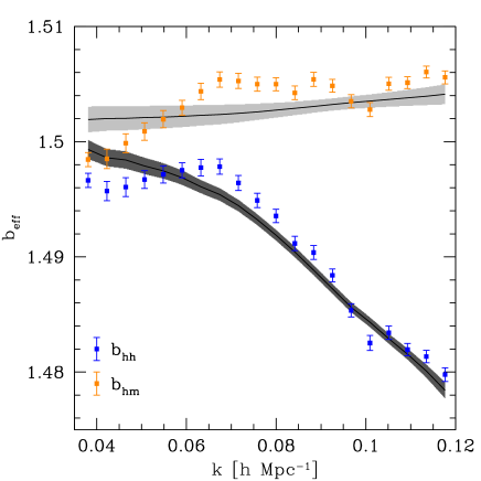
Figure 5: The effective halo-bias parameters bhm=Phm/Pmmsubscript𝑏hmsubscript𝑃hmsubscript𝑃mmb_{\rm hm}=P_{\rm hm}/P_{\rm mm} (orange symbols) and bhh=(Phh/Pmm)1/2subscript𝑏hhsuperscriptsubscript𝑃hhsubscript𝑃mm12b_{\rm hh}=(P_{\rm hh}/P_{\rm mm})^{1/2} (blue symbols) extracted from our simulations as a function of the wavenumber. The black solid lines and shaded regions indicate the mean and the rms value of the effective bias obtained by averaging the predictions of the second-order LEB over the posterior probability of the model parameters.
Refer to caption
Refer to caption
Refer to caption
Figure 6: Joint marginal probability distribution for the parameter pairs b1subscript𝑏1b_{1}–b2subscript𝑏2b_{2}, b1subscript𝑏1b_{1}–R𝑅R and b2subscript𝑏2b_{2}–R𝑅R (from left to right) obtained using the fully non-linear model for Phhsubscript𝑃hhP_{\rm hh} (black) and Phmsubscript𝑃hmP_{\rm hm} (green). Contours correspond to the 68.3 and 95.4 per cent credible intervals.

5.4.1 Power spectra

The tree-level SPT models for the halo power spectra provide very poor fits to our data. The minimum Ο‡2superscriptπœ’2\chi^{2} value is much larger than the number of degrees of freedom, reaching Ο‡min2≃7465similar-to-or-equalssubscriptsuperscriptπœ’2min7465\chi^{2}_{\rm min}\simeq 7465 for Phmsubscript𝑃hmP_{\rm hm} and Ο‡min2≃139,821similar-to-or-equalssubscriptsuperscriptπœ’2min139821\chi^{2}_{\rm min}\simeq 139,821 for Phhsubscript𝑃hhP_{\rm hh}. These results may serve as indicators that halo biasing is non-linear and/or a result of the breakdown of linear SPT. To check the latter, we refit both spectra using Equation (48) but after replacing P(1,1)treesuperscriptsubscript𝑃11treeP_{(1,1)}^{\rm tree} with the fully non-linear matter power spectrum P(1,1)subscript𝑃11P_{(1,1)}. In this case, we acquire Ο‡min2≃3903similar-to-or-equalssubscriptsuperscriptπœ’2min3903\chi^{2}_{\rm min}\simeq 3903 for Phmsubscript𝑃hmP_{\rm hm} and Ο‡min2≃4442similar-to-or-equalssubscriptsuperscriptπœ’2min4442\chi^{2}_{\rm min}\simeq 4442 for Phhsubscript𝑃hhP_{\rm hh}. This significant improvement to the tree-level results demonstrates the need to model non-linearities in the matter distribution very accurately. Using the fully non-linear model with the additional free-parameters b2subscript𝑏2b_{2} and R𝑅R only slightly improves the goodness of fit for Phmsubscript𝑃hmP_{\rm hm}, giving Ο‡min2≃3901similar-to-or-equalssubscriptsuperscriptπœ’2min3901\chi^{2}_{\rm min}\simeq 3901. On the other hand, the improvement is marked for Phhsubscript𝑃hhP_{\rm hh} for which we obtain Ο‡min2≃3915similar-to-or-equalssubscriptsuperscriptπœ’2min3915\chi^{2}_{\rm min}\simeq 3915.

It is interesting to see how the Ο‡min2subscriptsuperscriptπœ’2min\chi^{2}_{\rm min} value changes when R𝑅R is kept fixed. In this case, we find that all the fits to Phmsubscript𝑃hmP_{\rm hm} are equally good. However, for Phhsubscript𝑃hhP_{\rm hh}, the values of Ο‡min2subscriptsuperscriptπœ’2min\chi^{2}_{\rm min} undergo a sharp decrease (from 3944≲χmin2≲3921less-than-or-similar-to3944subscriptsuperscriptπœ’2minless-than-or-similar-to39213944\lesssim\chi^{2}_{\rm min}\lesssim 3921) for 2<R≲3.662𝑅less-than-or-similar-to3.662<R\lesssim 3.66 hβˆ’1​Mpcsuperscriptβ„Ž1Mpc\,h^{-1}{\rm Mpc}, then decrease slowly to the absolute minimum value at R∼13.2similar-to𝑅13.2R\sim 13.2 hβˆ’1​Mpcsuperscriptβ„Ž1Mpc\,h^{-1}{\rm Mpc} and finally begin to slowly rise again to our cutoff scale of R=18𝑅18R=18 hβˆ’1​Mpcsuperscriptβ„Ž1Mpc\,h^{-1}{\rm Mpc}. Hence, it appears that there is a range of preferred smoothing scales that best fit the simulation data for Phhsubscript𝑃hhP_{\rm hh}.

5.4.2 Bispectra

Turning now to the bispectra, we find that the fully non-linear model provides slightly better fits to the numerical data (Ο‡min2≃3906,3908similar-to-or-equalssubscriptsuperscriptπœ’2min39063908\chi^{2}_{\rm min}\simeq 3906,3908 and 391339133913 for Bhmmsubscript𝐡hmmB_{\rm hmm}, Bhhmsubscript𝐡hhmB_{\rm hhm}, and Bhhhsubscript𝐡hhhB_{\rm hhh}, respectively) than the tree-level model (Ο‡min2≃3923,3922similar-to-or-equalssubscriptsuperscriptπœ’2min39233922\chi^{2}_{\rm min}\simeq 3923,3922 and 392539253925) which, however, already supplies Ο‡min2/ν≲1less-than-or-similar-tosubscriptsuperscriptπœ’2min𝜈1\chi^{2}_{\rm min}/\nu\lesssim 1.

In all cases, if we keep R𝑅R fixed and only consider 2-parameter models, we find that the Ο‡min2subscriptsuperscriptπœ’2min\chi^{2}_{\rm min} value does not change much for 2<R<132𝑅132<R<13 hβˆ’1​Mpcsuperscriptβ„Ž1Mpc\,h^{-1}{\rm Mpc} while it rapidly grows adopting larger smoothing scales. In terms of goodness of fit, the non-linear model for Bhmmsubscript𝐡hmmB_{\rm hmm} outperforms the tree-level SPT model for all values of R𝑅R. On the other hand, when Bhhmsubscript𝐡hhmB_{\rm hhm} and Bhhhsubscript𝐡hhhB_{\rm hhh} are considered, the non-linear model gives a better fit only for R≲15less-than-or-similar-to𝑅15R\lesssim 15 hβˆ’1​Mpcsuperscriptβ„Ž1Mpc\,h^{-1}{\rm Mpc}.

5.4.3 Posterior mean

In order to give a visual impression of the best-fit models, in Figure 1 we show the posterior mean (black line) and the posterior rms error (shaded gray region) for the halo power and bispectra resulting from our fits with the fully non-linear model in comparison with the simulation data. In all cases, the models agree with the simulations remarkably well. Note that the rms error on the best-fit models for Phhsubscript𝑃hhP_{\rm hh} and Phmsubscript𝑃hmP_{\rm hm} is hardly visible on the scale of the plots.

5.5 Bias from the power spectrum

5.5.1 Effective bias

Due to its highly compressed ordinate, Figure 1 gives the false impression that Phmsubscript𝑃hmP_{\rm hm} and Phhsubscript𝑃hhP_{\rm hh} are nicely described by rescaling the matter power spectrum with constant multiplicative factors ∼1.5similar-toabsent1.5\sim 1.5 and 1.52superscript1.521.5^{2}, respectively. In order to examine the bias relation more closely as a function of scale, we introduce two effective bias coefficients by taking different ratios of the halo power spectra after111Very similar results are obtained if one averages the ratios instead of taking the ratio of the averages. averaging them over the 200 N-body simulations: bhm=⟨Phm⟩/⟨Pmm⟩subscript𝑏hmdelimited-⟨⟩subscript𝑃hmdelimited-⟨⟩subscript𝑃mmb_{\rm hm}=\langle P_{\rm hm}\rangle/\langle P_{\rm mm}\rangle and bhh=(⟨Phh⟩/⟨Pmm⟩)1/2subscript𝑏hhsuperscriptdelimited-⟨⟩subscript𝑃hhdelimited-⟨⟩subscript𝑃mm12b_{\rm hh}=(\langle P_{\rm hh}\rangle/\langle P_{\rm mm}\rangle)^{1/2}. We present our results in FigureΒ 5. The solid points with errorbars represent the effective biases estimated using the shot-noise corrected quantities of both the auto- and cross halo power spectra. We compute the 1​σ1𝜎1\sigma uncertainties via error propagation accounting for the covariance between the different observables. It can be seen that bhhsubscript𝑏hhb_{\rm hh} and bhmsubscript𝑏hmb_{\rm hm} do not perfectly match each other. On large-scales (k<0.06​h​Mpcβˆ’1π‘˜0.06β„ŽsuperscriptMpc1k<0.06\,\,h\,{\rm Mpc}^{-1}), bhhsubscript𝑏hhb_{\rm hh} keeps roughly constant while it shows a significant scale dependence for k>0.06​h​Mpcβˆ’1π‘˜0.06β„ŽsuperscriptMpc1k>0.06\,\,h\,{\rm Mpc}^{-1}, whereas bhmsubscript𝑏hmb_{\rm hm} shows the opposite trend although its scale dependence is weaker for the large scales. At k≃0.04​h​Mpcβˆ’1similar-to-or-equalsπ‘˜0.04β„ŽsuperscriptMpc1k\simeq 0.04\,\,h\,{\rm Mpc}^{-1}, bhmsubscript𝑏hmb_{\rm hm} and bhhsubscript𝑏hhb_{\rm hh} assume very similar values. However, bhm>bhhsubscript𝑏hmsubscript𝑏hhb_{\rm hm}>b_{\rm hh} for all wavenumbers. Our high-quality data also provide some hints for the presence of weak oscillatory features in the effective bias parameters on the scales of baryonic acoustic oscillations.

FigureΒ 5 also tests how the fully non-linear second-order LEB model is able to reproduce the scale-dependence of bhmsubscript𝑏hmb_{\rm hm} and bhhsubscript𝑏hhb_{\rm hh} in fine details. The black curves represent the posterior mean of the effective bias coefficients and the shaded grey regions denote the corresponding rms value of their posterior distribution. Although the models are not able to reproduce all the features which are present in the numerical data, they are in reasonable agreement with the simulations, especially for k>0.08​h​Mpcβˆ’1π‘˜0.08β„ŽsuperscriptMpc1k>0.08\,\,h\,{\rm Mpc}^{-1}. Nevertheless, we see that for both bhmsubscript𝑏hmb_{\rm hm} and bhhsubscript𝑏hhb_{\rm hh} the power spectum models actually are less accurate at small kπ‘˜k (i.e. on the large scales) in the proximity of the point where the trend from constant-to-scale dependence (and vice versa) occurs. On these scales, the models systematically overpredict the effective biases and the largest discrepancy is of the order of ∼0.3similar-toabsent0.3\sim 0.3 per cent.

Refer to caption
Figure 7: As in Figure 5 but for the effective bias parameters bhmm=Bhmm/Bmmmsubscript𝑏hmmsubscript𝐡hmmsubscript𝐡mmmb_{\rm hmm}=B_{\rm hmm}/B_{\rm mmm}, bhhm=(Bhhm/Bmmm)1/2subscript𝑏hhmsuperscriptsubscript𝐡hhmsubscript𝐡mmm12b_{\rm hhm}=(B_{\rm hhm}/B_{\rm mmm})^{1/2} and bhhh=(Bhhh/Bmmm)1/3subscript𝑏hhhsuperscriptsubscript𝐡hhhsubscript𝐡mmm13b_{\rm hhh}=(B_{\rm hhh}/B_{\rm mmm})^{1/3}.

5.5.2 Marginal credible regions

Now we compare the level of the consistency between the model-parameter constraints deriving from the fits to the halo power spectra, Phhsubscript𝑃hhP_{\rm hh} and Phmsubscript𝑃hmP_{\rm hm}. FigureΒ 6 shows (from left to right) the marginal posterior distributions for the parameter pairs b1subscript𝑏1b_{1}–b2subscript𝑏2b_{2}, b1subscript𝑏1b_{1}–R𝑅R and b2subscript𝑏2b_{2}–R𝑅R of our fully non-linear model. The black and green contours denote the 68.3%percent68.368.3\% and 95.4%percent95.495.4\% credible regions for the parameters of the LEB obtained from analyzing Phhsubscript𝑃hhP_{\rm hh} and Phmsubscript𝑃hmP_{\rm hm}, respectively. The first apparent observation is that the contours of Phmsubscript𝑃hmP_{\rm hm} and Phhsubscript𝑃hhP_{\rm hh} span different regions of the parameter space: while the Phmsubscript𝑃hmP_{\rm hm} data prefer b1≲1.5less-than-or-similar-tosubscript𝑏11.5b_{1}\lesssim 1.5 and b2≳0greater-than-or-equivalent-tosubscript𝑏20b_{2}\gtrsim 0, Phhsubscript𝑃hhP_{\rm hh} favours b1≳1.5greater-than-or-equivalent-tosubscript𝑏11.5b_{1}\gtrsim 1.5 combined with βˆ’0.15≲b2β‰²βˆ’0.2less-than-or-similar-to0.15subscript𝑏2less-than-or-similar-to0.2-0.15\lesssim b_{2}\lesssim-0.2. In other words, the second-order LEB model provides a succesful fit to Phhsubscript𝑃hhP_{\rm hh} or Phmsubscript𝑃hmP_{\rm hm} but requires two incompatible parameter sets. Improper modelling of the shot noise in Phhsubscript𝑃hhP_{\rm hh} might be the primary cause of the inconsistency (e.g. Hamaus etΒ al., 2010). Note, however, that the best-fit values for b1subscript𝑏1b_{1} and b2subscript𝑏2b_{2} that we derive from Phhsubscript𝑃hhP_{\rm hh} are in good agreement with the predictions of theories that follow the collapse of dark-matter halos (e.g. Equation (14) and (15) in Scoccimarro etΒ al., 2001). It is also worth mentioning that, for Gaussian fluctuations in the matter density, the cross-spectrum of locally-biased tracers is always exactly proportional to Pmmsubscript𝑃mmP_{\rm mm} even though this is not apparent from the mathematical formulation of the LEB (Frusciante & Sheth, 2012). The fact that our measurement of Phmsubscript𝑃hmP_{\rm hm} needs b2≃0similar-to-or-equalssubscript𝑏20b_{2}\simeq 0 might simply suggest that a similar relation holds true also in the presence of non-Gaussian perturbations (at least approximately, since bhmsubscript𝑏hmb_{\rm hm} keeps nearly constant with kπ‘˜k as shown in Fig. 5).

5.6 Bias from the bispectrum

5.6.1 Effective bias

To investigate the bias relation as a function of scale using the halo bispectra, we define a set of coefficients by taking the following ratios: bhmm=⟨Bhmm⟩200/⟨Bmmm⟩200subscript𝑏hmmsubscriptdelimited-⟨⟩subscript𝐡hmm200subscriptdelimited-⟨⟩subscript𝐡mmm200b_{\rm hmm}=\langle B_{\rm hmm}\rangle_{200}/\langle B_{\rm mmm}\rangle_{200}, bhhm=(⟨Bhhm⟩200/⟨Bmmm⟩200)1/2subscript𝑏hhmsuperscriptsubscriptdelimited-⟨⟩subscript𝐡hhm200subscriptdelimited-⟨⟩subscript𝐡mmm20012b_{\rm hhm}=(\langle B_{\rm hhm}\rangle_{200}/\langle B_{\rm mmm}\rangle_{200})^{1/2}, bhhh=(⟨Bhhh⟩200/⟨Bmmm⟩200)1/3subscript𝑏hhhsuperscriptsubscriptdelimited-⟨⟩subscript𝐡hhh200subscriptdelimited-⟨⟩subscript𝐡mmm20013b_{\rm hhh}=(\langle B_{\rm hhh}\rangle_{200}/\langle B_{\rm mmm}\rangle_{200})^{1/3}. The results are shown in Figure 7: all the effective bias coefficients present a characteristic configuration dependence and are in agreement within their 1​σ1𝜎1\sigma uncertainties (although bhhhsubscript𝑏hhhb_{\rm hhh} tends to assume slightly higher values for all triangle configurations). The posterior means of the effective bias coefficients from the fully non-linear models also closely match the data as expected from the Ο‡2superscriptπœ’2\chi^{2} test presented in Β§5.4.2. All this suggests the second-order LEB provides a suitable description of the bias relation at the three-point level.

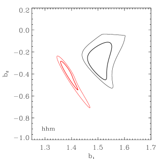
Refer to caption
Refer to caption
Refer to caption
Refer to caption
Refer to caption
Refer to caption
Refer to caption
Refer to caption
Refer to caption
Figure 8: Joint marginal probability distribution for the parameter pairs b1subscript𝑏1b_{1}–b2subscript𝑏2b_{2} (top), b1subscript𝑏1b_{1}–R𝑅R (middle) and b2subscript𝑏2b_{2}–R𝑅R (bottom) obtained fitting the data for Bhhhsubscript𝐡hhhB_{\rm hhh} (left), Bhhmsubscript𝐡hhmB_{\rm hhm} (center) and Bhmmsubscript𝐡hmmB_{\rm hmm} (right). Contours correspond to the 68.3 and 95.4 per cent credible intervals and refer to the full non-linear model (black) and to the approximation based on tree-level SPT (red).

5.6.2 Marginal credible regions

We now evaluate the consistency of the model-parameter constraints for the halo bispectra. FigureΒ 8 shows the marginal posterior distribution for the parameter pairs b1subscript𝑏1b_{1}–b2subscript𝑏2b_{2}, b1subscript𝑏1b_{1}–R𝑅R and b2subscript𝑏2b_{2}–R𝑅R, respectively. Each panel refers to a particular bispectrum, as indicated from the label in the bottom left corner. The black contours denote the 68.3%percent68.368.3\% and 95.4%percent95.495.4\% credible regions for the parameters of the fully non-linear model. The red contours, instead, indicate the corresponding regions for the SPT tree-level model described in Β§5.3.1.

The first thing that may be noticed is that the estimates for b1subscript𝑏1b_{1} and b2subscript𝑏2b_{2} from the tree-level and fully non-linear models are in disagreement: the tree-level constraints show a systematic shift, preferring lower b1subscript𝑏1b_{1} and slightly more negative b2subscript𝑏2b_{2} values. This implies that inferences made about the non-linearity of galaxy bias using the galaxy bispectrum and tree-level perturbation theory will be significantly biased. Note that this statement also applies to rather large scales k1≲0.12​h​Mpcβˆ’1less-than-or-similar-tosubscriptπ‘˜10.12β„ŽsuperscriptMpc1k_{1}\lesssim 0.12\,h\,{\rm Mpc}^{-1}. If one uses triangle configurations on smaller scales (e.g. Verde etΒ al., 2002) then the discrepancy becomes larger. Therefore, our program to use N-body simulations for determining the matter terms in the bias relation is key to correctly estimate the bias (and thus the cosmological parameters) from forthcoming observational data.

The second important point to notice is that fits to Bhhhsubscript𝐡hhhB_{\rm hhh}, Bhhmsubscript𝐡hhmB_{\rm hhm} and Bhmmsubscript𝐡hmmB_{\rm hmm} with the fully non-linear model give consistent constraints for b1subscript𝑏1b_{1}, b2subscript𝑏2b_{2} and R𝑅R. The precision with which we are able to determine the bias parameters increases as we go from Bhmmsubscript𝐡hmmB_{\rm hmm} to Bhhhsubscript𝐡hhhB_{\rm hhh}. This finding is consistent with our earlier results (Pollack, Smith & Porciani, 2012).

Note that the best-fit values for b1subscript𝑏1b_{1} appear relatively insensitive to variations in R𝑅R. One has to consider rather large smoothing scales in order to see any changes in the best-fit models. However, the best-fit solutions for b2subscript𝑏2b_{2} are strongly degenerate with R𝑅R: as R𝑅R decreases, b2subscript𝑏2b_{2} becomes less negative and tends towards zero. This owes to the fact that, on changing R𝑅R in the interval R∈[2,13]​hβˆ’1​Mpc𝑅213superscriptβ„Ž1MpcR\in[2,13]\,h^{-1}{\rm Mpc}, one can always find different combinations of b1subscript𝑏1b_{1} and b2subscript𝑏2b_{2} that fit the data with the same accuracy as previously described in 5.4. We can more directly understand the origin of the b2subscript𝑏2b_{2}–R𝑅R degeneracy as follows. Let us consider the bias model for Bhmmsubscript𝐡hmmB_{\rm hmm} since this only contains the terms ℬ(1,1,1)(s)subscriptsuperscriptℬs111{\mathcal{B}}^{\rm(s)}_{(1,1,1)} and ℬ(2,1,1)(s)subscriptsuperscriptℬs211{\mathcal{B}}^{\rm(s)}_{(2,1,1)}. As shown in the top panels of Fig. 4, the de-smoothing of ℬ(1,1,1)(s)subscriptsuperscriptℬs111{\mathcal{B}}^{\rm(s)}_{(1,1,1)} results in the matter bispectrum. However, the de-smoothing of ℬ(2,1,1)(s)subscriptsuperscriptℬs211{\mathcal{B}}^{\rm(s)}_{(2,1,1)} results in a function that carries a dependence on R𝑅R. If we take the ratio of ℬ(2,1,1)(s)subscriptsuperscriptℬs211{\mathcal{B}}^{\rm(s)}_{(2,1,1)} defined for Rasubscript𝑅aR_{\rm a} with the same function but defined for Rbsubscript𝑅bR_{\rm b}, then we will find something close to a constant for R=[4,10]​hβˆ’1​Mpc𝑅410superscriptβ„Ž1MpcR=[4,10]\,h^{-1}{\rm Mpc}. Thus we can identify the degenerate combination:

b2a=ℬ(2,1,1)(s)​(𝐀1,𝐀2,Rb)ℬ(2,1,1)(s)​(𝐀1,𝐀2,Ra)​b2bβ‰ˆA​(Ra,Rb)​b2bsuperscriptsubscript𝑏2asubscriptsuperscriptℬs211subscript𝐀1subscript𝐀2subscript𝑅bsubscriptsuperscriptℬs211subscript𝐀1subscript𝐀2subscript𝑅asuperscriptsubscript𝑏2b𝐴subscript𝑅asubscript𝑅bsuperscriptsubscript𝑏2bb_{2}^{\rm a}=\frac{{\mathcal{B}}^{\rm(s)}_{(2,1,1)}({\bf k}_{1},{\bf k}_{2},R_{\rm b})}{{\mathcal{B}}^{\rm(s)}_{(2,1,1)}({\bf k}_{1},{\bf k}_{2},R_{\rm a})}\,b_{2}^{\rm b}\approx A(R_{\rm a},R_{\rm b})\,b_{2}^{\rm b} (53)

where A​(Ra,Rb)𝐴subscript𝑅asubscript𝑅bA(R_{\rm a},R_{\rm b}) is a function that is independent of the triangle configuration. Hence, the value of b2subscript𝑏2b_{2} is correlated with the size of the smoothing scale, R𝑅R.

Refer to caption
Figure 9: Marginal probability distributions for the single bias parameters b1subscript𝑏1b_{1} (left), b2subscript𝑏2b_{2} (center) and R𝑅R (right) obtained fitting various halo statistics (from top to bottom: Phh,Phm,Bhhh,Bhhm,Bhmmsubscript𝑃hhsubscript𝑃hmsubscript𝐡hhhsubscript𝐡hhmsubscript𝐡hmmP_{\rm hh},P_{\rm hm},B_{\rm hhh},B_{\rm hhm},B_{\rm hmm}). Results obtained with the full non-linear model (black) are compared with those derived using tree-level SPT (red).

5.7 Comparing all constraints

Table 2: Posterior mean and rms error of the bias parameters b1subscript𝑏1b_{1}, b2subscript𝑏2b_{2} and R𝑅R obtained fitting various halo statistics with the full non-linear bias model.
Statistic b1Β±Οƒb1plus-or-minussubscript𝑏1subscript𝜎subscript𝑏1b_{1}\pm\sigma_{b_{1}} b2Β±Οƒb2plus-or-minussubscript𝑏2subscript𝜎subscript𝑏2b_{2}\pm\sigma_{b_{2}} RΒ±ΟƒRplus-or-minus𝑅subscriptπœŽπ‘…R\pm\sigma_{R}
(hβˆ’1​Mpcsuperscriptβ„Ž1Mpc\,h^{-1}{\rm Mpc})
Phhsubscript𝑃hhP_{\rm hh} 1.53 Β±plus-or-minus\pm 0.02 -0.18 Β±plus-or-minus\pm 0.02 12.0 Β±plus-or-minus\pm 3.1
Phmsubscript𝑃hmP_{\rm hm} 1.48 Β±plus-or-minus\pm 0.02 0.02 Β±plus-or-minus\pm 0.01 10.6 Β±plus-or-minus\pm 4.1
Bhhhsubscript𝐡hhhB_{\rm hhh} 1.49 ±plus-or-minus\pm 0.03 -0.18 ±plus-or-minus\pm 0.07 7.2 ±plus-or-minus\pm 2.6
Bhhmsubscript𝐡hhmB_{\rm hhm} 1.51 ±plus-or-minus\pm 0.03 -0.26 ±plus-or-minus\pm 0.10 7.8 ±plus-or-minus\pm 2.8
Bhmmsubscript𝐡hmmB_{\rm hmm} 1.52 ±plus-or-minus\pm 0.05 -0.31 ±plus-or-minus\pm 0.14 9.1 ±plus-or-minus\pm 3.1

In FigureΒ 9 we present the marginal posterior probabilities for the single bias parameters extracted from the various probes that we have considered. The left, central and middle columns show the results for b1subscript𝑏1b_{1}, b2subscript𝑏2b_{2} and R𝑅R, respectively. From top to bottom, the rows correspond to Phh,Phm,Bhhhsubscript𝑃hhsubscript𝑃hmsubscript𝐡hhhP_{\rm hh},P_{\rm hm},B_{\rm hhh}, Bhhm,Bhmmsubscript𝐡hhmsubscript𝐡hmmB_{\rm hhm},B_{\rm hmm}, respectively. The black curves represent the results from the fully non-linear modelling, and the red curves show the results from the tree-level perturbation theory for the bispectra. The corresponding mean and rms values of the marginal probabilities for the full non-linear model are reported in Table 2.

Considering the values for b1subscript𝑏1b_{1} from the bispectra, we see that, as noted earlier, the parameter constraints for the non-linear model are consistent with one another and are significantly different from the best-fit b1subscript𝑏1b_{1} obtained from the tree-level expressions. On comparing the bispectra results with the power-spectra results we find reasonable consistency for the non-linear modelling, whereas for the tree-level bispectrum model, the results disagree at high significance (see also Pollack, Smith & Porciani, 2012). However, the marginal distributions for b1subscript𝑏1b_{1} from Phhsubscript𝑃hhP_{\rm hh} and Phmsubscript𝑃hmP_{\rm hm} overlap very little. In fact, they exhibit opposite skewness although they are both narrow and located around b1≃1.5similar-to-or-equalssubscript𝑏11.5b_{1}\simeq 1.5. The marginal distribution for b1subscript𝑏1b_{1} computed from Phmsubscript𝑃hmP_{\rm hm} agrees remarkably well with the effective bias bhm=1.503Β±0.002subscript𝑏hmplus-or-minus1.5030.002b_{\rm hm}=1.503\pm 0.002. This is because the data require b2≃0similar-to-or-equalssubscript𝑏20b_{2}\simeq 0 in this case. On the other hand, b1>bhh=1.49Β±0.002subscript𝑏1subscript𝑏hhplus-or-minus1.490.002b_{1}>b_{\rm hh}=1.49\pm 0.002 in the marginal distribution extracted from Phhsubscript𝑃hhP_{\rm hh} which requires b2<0subscript𝑏20b_{2}<0.

Examining the results of the fully non-linear model for b2subscript𝑏2b_{2}, from the bispectra we find that the marginal posterior distributions are fairly broad and are peaked towards negative values (b2β‰ƒβˆ’0.2similar-to-or-equalssubscript𝑏20.2b_{2}\simeq-0.2 for Bhhhsubscript𝐡hhhB_{\rm hhh}, b2β‰ƒβˆ’0.3similar-to-or-equalssubscript𝑏20.3b_{2}\simeq-0.3 for Bhhmsubscript𝐡hhmB_{\rm hhm} and Bhmmsubscript𝐡hmmB_{\rm hmm}). Overall, the various bispectra give consistent constraints. Note that the sharp cutoff in the marginal distributions at b2≃0similar-to-or-equalssubscript𝑏20b_{2}\simeq 0 is due to the fact that our prior for R𝑅R does not consider values R<2​hβˆ’1​Mpc𝑅2superscriptβ„Ž1MpcR<2\,h^{-1}{\rm Mpc}. Considering the results obtained using the tree-level SPT model, we see that the distributions for b1subscript𝑏1b_{1} and b2subscript𝑏2b_{2} shift towards different values (approximately the posterior mean of the bias parameters moves by Δ​b1≃Δ​b2β‰ƒβˆ’0.15similar-to-or-equalsΞ”subscript𝑏1Ξ”subscript𝑏2similar-to-or-equals0.15\Delta b_{1}\simeq\Delta b_{2}\simeq-0.15). On comparing with the results obtained from the halo power spectra, we see that the marginal distribution for b2subscript𝑏2b_{2} extracted from Phhsubscript𝑃hhP_{\rm hh} and Phmsubscript𝑃hmP_{\rm hm} are narrowly peaked around b2βˆΌβˆ’0.18similar-tosubscript𝑏20.18b_{2}\sim-0.18 and b2∼0.02similar-tosubscript𝑏20.02b_{2}\sim 0.02, respectively.

We now turn to the question of whether there is a preferred smoothing scale for the haloes we have considered. On inspecting the bispectra, we see that the marginal distributions for R𝑅R are reasonably consistent and display a broad peak between 5 and 12 hβˆ’1​Mpcsuperscriptβ„Ž1Mpc\,h^{-1}{\rm Mpc}. The power spectra, instead, tend to prefer slighty larger values of R𝑅R: 10<R<15​hβˆ’1​Mpc10𝑅15superscriptβ„Ž1Mpc10<R<15\,h^{-1}{\rm Mpc} for Phhsubscript𝑃hhP_{\rm hh} and R>5​hβˆ’1​Mpc𝑅5superscriptβ„Ž1MpcR>5\,h^{-1}{\rm Mpc} for Phmsubscript𝑃hmP_{\rm hm}, consistent with the behaviour of the goodness of fit reported in Β§5.4. In all cases, these optimal smoothing scales correspond to a few Lagrangian radii of the halos. They are also comparable to (but a bit smaller than) the scales that we sample with the measurements of the power spectra and bispectra. Note that a sphere of radius ∼10​hβˆ’1​Mpcsimilar-toabsent10superscriptβ„Ž1Mpc\sim 10\,h^{-1}{\rm Mpc} contains ∼1.5similar-toabsent1.5\sim 1.5 halos on average so that counts in cells of this extension are subject to sizable random fluctuations that create stochasticity in the bias relation.

5.8 Cross-correlation coefficients

There are three possible explanations as to why Phmsubscript𝑃hmP_{\rm hm}, Phhsubscript𝑃hhP_{\rm hh} and the bispectra show disagreement for the full non-linear model. One, we may require higher-order terms in the bias expansion, e.g. b3subscript𝑏3b_{3} etc; two, the LEB may be wrong; three, there may be uncorrelated stochasticity in the relation between halo overdensity and mass overdensity. We shall now explore this latter possibility.

A number of studies have demonstrated, using N𝑁N-body simulations, that the relation between Ξ΄h​(𝐱|R)subscript𝛿hconditional𝐱𝑅\delta_{\rm h}({\bf x}|R) against δ​(𝐱|R)𝛿conditional𝐱𝑅\delta({\bf x}|R) contains scatter, and that this scatter depends on the scale which one uses to compute the density field (e.g. Dekel & Lahav, 1999; Seljak & Warren, 2004; Smith, Scoccimarro & Sheth, 2007; Manera & GaztaΓ±aga, 2011; Roth & Porciani, 2011; Pollack, Smith & Porciani, 2012; Chuen Chan & Scoccimarro, 2012).
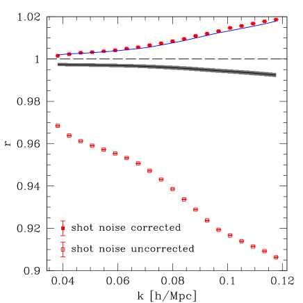
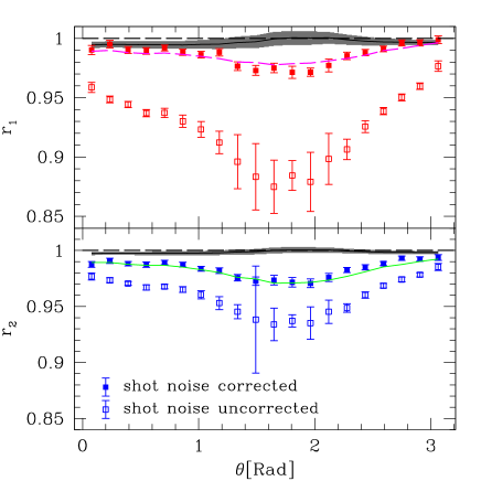
Refer to caption
Refer to caption
Figure 10: Left: Linear cross-correlation coefficient between the fluctuations in the halo and matter density, r=bhm/bhhπ‘Ÿsubscript𝑏hmsubscript𝑏hhr=b_{\rm hm}/b_{\rm hh}, for different wavenumbers. Closed and open symbols show the results obtained from the simulations when Phhsubscript𝑃hhP_{\rm hh} is and is not corrected for shot noise, respectively. The black solid line and the shaded region around it indicate the mean and the rms value of the correlation coefficient obtained by averaging the predictions of the second-order LEB over the posterior probability of the model parameters derived from a joint fit to Phhsubscript𝑃hhP_{\rm hh} and Phmsubscript𝑃hmP_{\rm hm}. The solid curve, instead, shows the values of rπ‘Ÿr that are computed using the means for Phhsubscript𝑃hhP_{\rm hh} and Phmsubscript𝑃hmP_{\rm hm} over the posterior distributions for the individual fits to Phhsubscript𝑃hhP_{\rm hh} and Phmsubscript𝑃hmP_{\rm hm}, respectively. Right: As in the left panel but for the 3-point coefficients r1subscriptπ‘Ÿ1r_{1} and r2subscriptπ‘Ÿ2r_{2} defined in Equations (58) and (59). In this case, the shaded region is obtained averaging the model over the posterior distribution for the parameters derived from a joint fit to the relevant bispectra, while the solid curve uses the different means from the fits to the individual bispectra.

Another way to explore the stochasticity is through the cross-correlation coefficient between Fourier modes. For two-point statistics this can be defined (Dekel & Lahav, 1999):

r≑P^hmP^hh​P^mm=bhmbhh.π‘Ÿsubscript^𝑃hmsubscript^𝑃hhsubscript^𝑃mmsubscript𝑏hmsubscript𝑏hhr\equiv\frac{\hat{P}_{\rm hm}}{\sqrt{\hat{P}_{\rm hh}\hat{P}_{\rm mm}}}=\frac{b_{\rm hm}}{b_{\rm hh}}\ . (54)

If Ξ΄hsuperscript𝛿h\delta^{\rm h} is a deterministic linear function of δ𝛿\delta, then r=Β±1π‘Ÿplus-or-minus1r=\pm 1. However, if there is uncorrelated random noise present, i.e. Ξ΄h​(𝐱)=b​δ​(𝐱)+ϡ​(𝐱)superscript𝛿h𝐱𝑏𝛿𝐱italic-ϡ𝐱\delta^{\rm h}({\bf x})=b\delta({\bf x})+\epsilon({\bf x}), then the halo power spectrum would be Phh​(k)=b2​Pmm​(k)+Pϡ​(k)subscript𝑃hhπ‘˜superscript𝑏2subscript𝑃mmπ‘˜subscript𝑃italic-Ο΅π‘˜P_{\rm hh}(k)=b^{2}P_{\rm mm}(k)+P_{\epsilon}(k), where PΟ΅subscript𝑃italic-Ο΅P_{\epsilon} denotes the power spectrum of the noise distribution. This leads to:

r=(1+PΟ΅Pmm)βˆ’1/2<1.π‘Ÿsuperscript1subscript𝑃italic-Ο΅subscript𝑃mm121r=\left(1+\frac{P_{\epsilon}}{P_{\rm mm}}\right)^{-1/2}<1\ . (55)

We note that non-linearity in the bias relationship will also introduce deviations of rπ‘Ÿr away from unity: consider the quadratic relation Ξ΄h​(𝐱)=b1​δ​(𝐱)+b2​δ2​(𝐱)/2subscript𝛿h𝐱subscript𝑏1𝛿𝐱subscript𝑏2superscript𝛿2𝐱2\delta_{\rm h}({\bf x})=b_{1}\delta({\bf x})+b_{2}\,\delta^{2}({\bf x})/2, then one finds that the cross-correlation can be written:

rπ‘Ÿ\displaystyle r =\displaystyle= [1+c22​𝒫(2,1)𝒫(1,1)]​[1+c2​𝒫(2,1)𝒫(1,1)+c224​𝒫(2,2)𝒫(1,1)]βˆ’1/2delimited-[]1subscript𝑐22subscript𝒫21subscript𝒫11superscriptdelimited-[]1subscript𝑐2subscript𝒫21subscript𝒫11superscriptsubscript𝑐224subscript𝒫22subscript𝒫1112\displaystyle\left[1+\frac{c_{2}}{2}\frac{\mathcal{P}_{(2,1)}}{\mathcal{P}_{(1,1)}}\right]\left[1+c_{2}\frac{\mathcal{P}_{(2,1)}}{\mathcal{P}_{(1,1)}}+\frac{c_{2}^{2}}{4}\frac{{\mathcal{P}}_{(2,2)}}{{\mathcal{P}}_{(1,1)}}\right]^{-1/2} (56)
β‰ˆ\displaystyle\approx 1βˆ’c228​𝒫(2,2)𝒫(1,1).1superscriptsubscript𝑐228subscript𝒫22subscript𝒫11\displaystyle 1-\frac{c_{2}^{2}}{8}\frac{{\mathcal{P}}_{(2,2)}}{{\mathcal{P}}_{(1,1)}}\ . (57)

where c2≑b2/b1subscript𝑐2subscript𝑏2subscript𝑏1c_{2}\equiv b_{2}/b_{1} and where the second equality follows for the case where 𝒫(2,1)β‰ͺ𝒫(1,1)much-less-thansubscript𝒫21subscript𝒫11{\mathcal{P}}_{(2,1)}\ll{\mathcal{P}}_{(1,1)} and 𝒫(2,2)β‰ͺ𝒫(1,1)much-less-thansubscript𝒫22subscript𝒫11{\mathcal{P}}_{(2,2)}\ll{\mathcal{P}}_{(1,1)}.

In this case, we see that the cross-correlation function can be either greater or less than unity depending on the sign and magnitude of c2subscript𝑐2c_{2}.

FigureΒ 10 shows the cross-correlation coefficient estimated from our ensemble of N𝑁N-body simulations along with the standard errors on the mean. The open symbols show the result before we correct Phhsubscript𝑃hhP_{\rm hh} for shot noise, the solid symbols show the result after the usual inverse number-density correction. We see that before correcting for the shot noise the function is less than 1 and decreases with scale. After the correction, rπ‘Ÿr is brought within a few percent from unity and is always larger than one. Note that the difference from unity is very significant given the numbers of realizations and the comoving volume covered by our simulations.

In order to derive rπ‘Ÿr from the fully non-linear model, we jointly fit the numerical data for Phmsubscript𝑃hmP_{\rm hm} and Phhsubscript𝑃hhP_{\rm hh}. We acknowledge that utilizing 200 simulations prevents us from accurately estimating a 40Γ—40404040\times 40 covariance matrix, in particular the cross covariances between the different spectra. Therefore, we performed the joint fit in the following manner. In order to ensure that the different spectra can be treated as independent of each other, we generated two ensembles consisting of 100 simulations each to estimate a particular spectra. We then computed a 20x20 block covariance matrix, selecting every other bin from our auto- and cross- power spectrum estimates. The off-diagonal blocks of the covariance matrix were set equal to zero when analyzing the auto-halo and cross halo-matter power spectrum. The resulting best-fit model (b1≃1.5,b2β‰ƒβˆ’0.09,R≃18formulae-sequencesimilar-to-or-equalssubscript𝑏11.5formulae-sequencesimilar-to-or-equalssubscript𝑏20.09similar-to-or-equals𝑅18b_{1}\simeq 1.5,b_{2}\simeq-0.09,R\simeq 18) does not match to the data (Ο‡min2≃2242/1997similar-to-or-equalssubscriptsuperscriptπœ’2min22421997\chi^{2}_{\rm min}\simeq 2242/1997 with a contribution of 1170 coming from Phmsubscript𝑃hmP_{\rm hm}) meaning that it is impossible to simultaneously fit Phhsubscript𝑃hhP_{\rm hh} and Phmsubscript𝑃hmP_{\rm hm} with the second-order LEB. Consequently, we find that the posterior mean of the cross-correlation coefficent, obtained by multiplying the likelihoods of the single fits to Phhsubscript𝑃hhP_{\rm hh} and Phmsubscript𝑃hmP_{\rm hm}, is always smaller than unity and does not provide a good description to the data (see the black line and the shaded region in FigureΒ 10). To investigate this further, we recompute rπ‘Ÿr using the posterior means of Phhsubscript𝑃hhP_{\rm hh} and Phmsubscript𝑃hmP_{\rm hm} shown in the left panel of FigureΒ 1. Inserting them in Equation (54), we find excellent agreement with the data (see the blue line in FigureΒ 1). As shown previously, the best-fit models for Phhsubscript𝑃hhP_{\rm hh} and Phmsubscript𝑃hmP_{\rm hm} prefer different values for b1subscript𝑏1b_{1} and b2subscript𝑏2b_{2} when analyzed independently. The joint analysis of Phmsubscript𝑃hmP_{\rm hm} and Phhsubscript𝑃hhP_{\rm hh}, in this manner, shows more clearly the inconsistency obtained when using the second-order LEB as a model for halo biasing.

One can also define cross-correlation coefficients for higher-order statistics. The second equality in Eq. (54) gives us a clear path to make this generalization. From the 3-point effective bias coefficients we may form two independent ratios:

r1subscriptπ‘Ÿ1\displaystyle r_{1} ≑\displaystyle\equiv bhmmbhhh=BhmmBmmm2/3​Bhhh1/3subscript𝑏hmmsubscript𝑏hhhsubscript𝐡hmmsuperscriptsubscript𝐡mmm23superscriptsubscript𝐡hhh13\displaystyle\frac{b_{\rm hmm}}{b_{\rm hhh}}=\frac{B_{\rm hmm}}{B_{\rm mmm}^{2/3}B_{\rm hhh}^{1/3}} (58)
r2subscriptπ‘Ÿ2\displaystyle r_{2} ≑\displaystyle\equiv bhhmbhhh=Bhhm1/2Bmmm1/6​Bhhh1/3,subscript𝑏hhmsubscript𝑏hhhsuperscriptsubscript𝐡hhm12superscriptsubscript𝐡mmm16superscriptsubscript𝐡hhh13\displaystyle\frac{b_{\rm hhm}}{b_{\rm hhh}}=\frac{B_{\rm hhm}^{1/2}}{B_{\rm mmm}^{1/6}B_{\rm hhh}^{1/3}}\ , (59)

where the dependence on the triangle configuration is understood. Note, that a third (dependent) ratio may be also computed: r3=bhmm/bhhm=r1/r2subscriptπ‘Ÿ3subscript𝑏hmmsubscript𝑏hhmsubscriptπ‘Ÿ1subscriptπ‘Ÿ2r_{3}=b_{\rm hmm}/b_{\rm hhm}=r_{1}/r_{2}. For a deterministic linear bias model with bias coefficient b𝑏b, r1=1subscriptπ‘Ÿ11r_{1}=1 and r2=sgn​(b)subscriptπ‘Ÿ2sgn𝑏r_{2}={\mathrm{sgn}}(b). Once again, additional stochasticity or non-linear biasing will alter the cross-correlation coefficients.

In the right panel of FigureΒ 10 we present the cross-correlation coefficients r1subscriptπ‘Ÿ1r_{1} and r2subscriptπ‘Ÿ2r_{2} extracted from the simulations as a function of the triangle configuration. Both functions are always a few per cent below unity even after shot-noise subtraction. In the same figure, we also plot the posterior mean and variance for the rπ‘Ÿr coefficients obtained from joint fits to two bispectra (black line and shaded region) performed in the same manner as for the power spectrum. These results are very close to unity and do not adequately describe the simulated data. In fact, the joint fits prefer less negative values for b2subscript𝑏2b_{2} than the single fits (for example, the best simultaneous fit to Bhhhsubscript𝐡hhhB_{\rm hhh} and Bhhmsubscript𝐡hhmB_{\rm hhm} gives b1≃1.50,b2β‰ƒβˆ’0.15formulae-sequencesimilar-to-or-equalssubscript𝑏11.50similar-to-or-equalssubscript𝑏20.15b_{1}\simeq 1.50,b_{2}\simeq-0.15 and R≃5.5similar-to-or-equals𝑅5.5R\simeq 5.5 with Ο‡min2/ν≃1954/1997similar-to-or-equalssubscriptsuperscriptπœ’2min𝜈19541997\chi^{2}_{\rm min}/\nu\simeq 1954/1997). On the other hand, if we compute r1subscriptπ‘Ÿ1r_{1} and r2subscriptπ‘Ÿ2r_{2} from the individual posterior means for Bhhhsubscript𝐡hhhB_{\rm hhh}, Bhhmsubscript𝐡hhmB_{\rm hhm} and Bhmmsubscript𝐡hmmB_{\rm hmm}, we get results that are in good agreement with the data. This is somewhat puzzling as the fits to the various bispectra appear to give consistent bias parameters. However, in order to test how congruous the different fits really are, we derive models for one bispectrum type (say Bhhhsubscript𝐡hhhB_{\rm hhh}) averaging over the joint posterior distribution for the bias parameters derived by fitting one of the other bispectra (Bhmmsubscript𝐡hmmB_{\rm hmm} or Bhhmsubscript𝐡hhmB_{\rm hhm}). An example is shown in FigureΒ 11: the fit based on Bhmmsubscript𝐡hmmB_{\rm hmm} matches well the data for Bhhhsubscript𝐡hhhB_{\rm hhh} for collinear triangles but systematically underestimates the halo bispectrum in all the other configurations. It is exactly in this more precise comparison that we see the failure of the non-linear local bias model when analyzing the bispectra data.
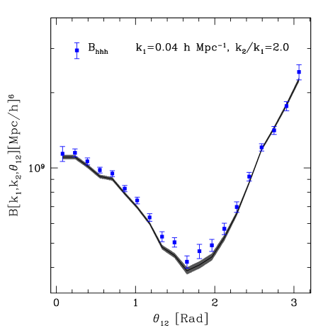
Refer to caption
Figure 11: The halo bispectrum, Bhhhsubscript𝐡hhhB_{\rm hhh}, measured from the simulations (solid symbols) is compared with the fully non-linear LEB adopting the parameters that best fit Bhmmsubscript𝐡hmmB_{\rm hmm}. The line and shaded region show the mean and rms value of the LEB model for Bhhhsubscript𝐡hhhB_{\rm hhh} averaged over the posterior distribution for b1,b2subscript𝑏1subscript𝑏2b_{1},b_{2} and R𝑅R coming from a fit to Bhmmsubscript𝐡hmmB_{\rm hmm}. This shows that the parameter sets that nicely fit Bhmmsubscript𝐡hmmB_{\rm hmm} (see Figure 1) are not able to reproduce all the features seen in Bhhhsubscript𝐡hhhB_{\rm hhh}.

6 Discussion

Our high-precision measurements of the halo-halo and halo-matter spectra and bispectra enabled us to carry out a series of consistency tests of the second-order LEB. As seen in Figure 9 and in Table 2, the marginal posterior distributions for b1subscript𝑏1b_{1} and b2subscript𝑏2b_{2} determined from Phh,Bhhh,Bhhmsubscript𝑃hhsubscript𝐡hhhsubscript𝐡hhmP_{\rm hh},B_{\rm hhh},B_{\rm hhm} and Bhmmsubscript𝐡hmmB_{\rm hmm} are all consistent with one another and, yet, are inconsistent with the constraints derived from the halo-matter cross spectrum. The primary reason is that Phmsubscript𝑃hmP_{\rm hm} requires a positive b2subscript𝑏2b_{2} that is close to 0, whereas the fits to the other spectra prefer a negative value for b2subscript𝑏2b_{2}. In terms of statistical significance, the stronger discrepancy is with Phhsubscript𝑃hhP_{\rm hh} as the posterior distributions for b2subscript𝑏2b_{2} extracted from all bispectra are rather broad. The incompatibility between the bias parameters obtained from Phhsubscript𝑃hhP_{\rm hh} and Phmsubscript𝑃hmP_{\rm hm} might indicate a breakdown in the modelling due to either incorrect shot-noise subtraction or incorrect parameterization of halo biasing. To better understand this issue, it is interesting to focus for a moment onto the shot-noise free spectra Phmsubscript𝑃hmP_{\rm hm} and Bhmmsubscript𝐡hmmB_{\rm hmm}. Comparing their mathematical expressions given in Equations (17) and (21), we see that they have the same parametric form in terms of b1subscript𝑏1b_{1} and b2subscript𝑏2b_{2}, it is only the non-linear matter terms which are different. Since we directly measure these terms from the simulations and shot-noise does not play any role here, the fact that the model-parameter constraints from Phmsubscript𝑃hmP_{\rm hm} and Bhmmsubscript𝐡hmmB_{\rm hmm} are incompatible suggests that the LEB truncated to second-order is incorrect or, at the very least, incomplete. The simplest improvement would be to consider higher-order terms in the bias expansion given in Equation (3). However, there are good reasons to believe that more sophisticated corrections are needed. Recent numerical work has provided strong evidence that dark-matter halos form out of linear density peaks (Ludlow & Porciani, 2011). This suggests that the halo bias with respect to the matter fluctuations may actually be best understood as originating in Lagrangian space (Catelan etΒ al., 1998; Catelan, Porciani & Kamionkowski, 2000). However, even the simplest local Lagrangian biasing scheme generates a non-linear, non-local and stochastic scheme in Eulerian space (Catelan etΒ al., 1998; Catelan, Porciani & Kamionkowski, 2000; Matsubara, 2011) which can be parameterized in terms of the invariants of the deformation tensor (Catelan etΒ al., 1998; Chan, Scoccimarro & Sheth, 2012; Baldauf etΒ al., 2012). Several terms should then be added to the bias expansion of the LEB and this might help bring the model-parameter constraints extracted from the different halo statistics in to better agreement. We will revisit this issue in our future work.

7 Conclusions

The use of galaxy clustering to extract information on the cosmological parameters is currently limited to very large scales where both galaxy biasing and the process of structure formation are expected to be linear and thus simple to model. Although more precise data are already available on smaller scales, they are not usually considered to avoid daunting complications in the modeling that might introduce systematic effects in the results. Pursuing the goal of extending clustering studies to smaller scales, we propose to use N-body simulations to measure the relevant statistics for the matter distribution that enter any biasing scheme.

While our framework is explicitly general, as an example, we apply it to the Eulerian local bias model truncated to quadratic order. This scheme represents the minimal theoretical model for studying three-point statistics of the galaxy distribution on large spatial separations. Its predictions are easily computed to leading order in SPT and are commonly used to interpret observational results (Verde etΒ al., 2002; Jing & BΓΆrner, 2004; Wang etΒ al., 2004; Kayo etΒ al., 2004; GaztaΓ±aga etΒ al., 2005; Hikage etΒ al., 2005; Pan & Szapudi, 2005; Kulkarni etΒ al., 2007; Nishimichi etΒ al., 2007; MarΓ­n, 2011; McBride etΒ al., 2011, 2011; Guo etΒ al., 2013; MarΓ­n etΒ al., 2013).

We use a set of 200 N𝑁N-body simulations to study the clustering properties of dark-matter halos and their relation to the underlying matter distribution with unprecedented accuracy. Our halo catalogs cover a total comoving volume of 675​hβˆ’3​Gpc3675superscriptβ„Ž3superscriptGpc3675\,h^{-3}\,{\rm Gpc}^{3}, much larger than the effective volume of the SDSS LRG sample (0.26​hβˆ’3​Gpc30.26superscriptβ„Ž3superscriptGpc30.26\,h^{-3}\,{\rm Gpc}^{3}), the BOSS BAO sample (2.4​hβˆ’3​Gpc32.4superscriptβ„Ž3superscriptGpc32.4\,h^{-3}\,{\rm Gpc}^{3}) and the planned spectroscopic survey of the Euclid satellite (19.7​hβˆ’3​Gpc319.7superscriptβ„Ž3superscriptGpc319.7\,h^{-3}\,{\rm Gpc}^{3}). We consider halos with mass M>1.11Γ—1013​hβˆ’1​MβŠ™π‘€1.11superscript1013superscriptβ„Ž1subscript𝑀direct-productM>1.11\times 10^{13}h^{-1}M_{\odot} corresponding to a number density of 3.7Γ—10βˆ’4​hβˆ’3​Mpc33.7superscript104superscriptβ„Ž3superscriptMpc33.7\times 10^{-4}\,h^{-3}\,{\rm Mpc}^{3} so that the effective volume (i.e. the actual volume weighted by the factor n¯​Phh¯𝑛subscript𝑃hh\bar{n}\,P_{\rm hh}) roughly coincides with the total volume for the wavenumbers analyzed here (0.04≲k≲0.12​h​Mpcβˆ’1less-than-or-similar-to0.04π‘˜less-than-or-similar-to0.12β„ŽsuperscriptMpc10.04\lesssim k\lesssim 0.12\,h\,{\rm Mpc}^{-1}) that match the observable scales of current and future surveys. All this allows us to measure the halo power spectrum to sub-percent accuracy (better than 0.3 per cent at k≃0.04​h​Mpcβˆ’1similar-to-or-equalsπ‘˜0.04β„ŽsuperscriptMpc1k\simeq 0.04\,h\,{\rm Mpc}^{-1}) and the halo bispectrum to a few per cent accuracy.

We make a twofold use of our simulations: to measure the moments of the non-linear matter distribution on several scales (and compare them against SPT predictions) and to test how well the LEB truncated to quadratic order fits several statistics of the halo distribution. In particular, we consider the halo power spectrum, Phhsubscript𝑃hhP_{\rm hh}, the halo-mass cross-spectrum, Phmsubscript𝑃hmP_{\rm hm}, as well as all the possible bispectra Bhhhsubscript𝐡hhhB_{\rm hhh}, Bhhmsubscript𝐡hhmB_{\rm hhm} and Bhmmsubscript𝐡hmmB_{\rm hmm}. Our main results can be summarized as follows:

  1. 1.

    In a ΛΛ\LambdaCDM model at z=0𝑧0z=0, tree-level SPT does not accurately model non-linearities in the momenta of the matter distribution on spatial scales of the order of 10βˆ’30​hβˆ’1​Mpc1030superscriptβ„Ž1Mpc10-30\,h^{-1}{\rm Mpc}.

  2. 2.

    The simple second-order LEB fits very well all halo spectra and bispectra when either N𝑁N-body simulations or tree-level SPT are used in the modelling of the clustering amplitudes for the matter distribution. However, the bias parameters derived from the models based on SPT are heavily biased with respect to the case when non-linearities are accurately modelled. This might explain why studies that interpreted different statistics of the galaxy distirbution based on SPT reached inconsistent conclusions regarding the non-linear bias of optically selected galaxies (e.g. Verde etΒ al., 2002; GaztaΓ±aga etΒ al., 2005).

  3. 3.

    The LEB models applied to counts in cells requires an optimal smoothing scale of several hβˆ’1​Mpcsuperscriptβ„Ž1Mpc\,h^{-1}{\rm Mpc} to match the halo statistics from the simulations. For our halos, this corresponds to a few Lagrangian radii but is also of the same order of the spatial scales under analysis.

  4. 4.

    Comparing the parameter constraints for the fully non-linear LEB obtained from the different spectra, we find some inconsistencies. In particular, the non-linear bias parameter extracted from the cross-spectrum Phmsubscript𝑃hmP_{\rm hm} is incompatible with the results from all the other statistics. The main difference is that Phmsubscript𝑃hmP_{\rm hm} strongly favours a positive value for b2subscript𝑏2b_{2} that is very close to zero, whereas the posterior distributions derived from all other spectra prefer a negative b2subscript𝑏2b_{2} in the range βˆ’0.3≲b2β‰²βˆ’0.2less-than-or-similar-to0.3subscript𝑏2less-than-or-similar-to0.2-0.3\lesssim b_{2}\lesssim-0.2. General agreement, instead, is found for the linear bias parameter, b1subscript𝑏1b_{1}.

  5. 5.

    Non-trivial shot-noise corrections in Phhsubscript𝑃hhP_{\rm hh} might be invoked to reconcile the bias-parameters extracted from Phmsubscript𝑃hmP_{\rm hm} and Phhsubscript𝑃hhP_{\rm hh}. However this cannot explain the differences between the constraints from the shot-noise free statistics Phmsubscript𝑃hmP_{\rm hm} and Bhmmsubscript𝐡hmmB_{\rm hmm}. This suggests that further complexity should be added to second-order LEB in order to match all halo statistics.

  6. 6.

    Analysis of the cross-correlation coefficients defined for the two-point and three-point statistics reveal further subtle inconsistencies contained in the LEB truncated to second order, suggesting it is too simple a model to describe halo bias with high accuracy.

A final remark is in order. Our numerical study is based on simulations with a fixed background cosmology and focuses on retrieving the bias parameters when the cosmological parameters are perfectly known. However, this is not the case for actual galaxy surveys where bias and cosmology are generally estimated simultaneously. To transform our method into a resourceful tool for data analysis, we will need to explore how the shapes and amplitudes of the moments of the non-linear matter density field depend on the unknown cosmological parameters without having to run an exorbitant amount of N𝑁N-body simulations (e.g. Angulo & White, 2010) – a topic we shall explore in future work.

Acknowledgements

JEP thanks Xun Shi and AndrΓ©s Balaguera-AntolΓ­nez for useful discussions. We thank V. Springel for making public GADGET-2 and for providing his B-FoF halo finder, and R.Β Scoccimarro for making public his 2LPT code. JEP and CP were partially supported by funding provided through the SFB-Transregio 33 β€œThe Dark Universe” by the Deutsche Forschungsgemeinschaft. RES acknowledges support from ERC Advanced Grant 246797 β€œGALFORMOD”.

References

  • Angulo & White (2010) Angulo R.Β E., White S.Β D.Β M., 2010, MNRAS, 405, 143
  • Baldauf etΒ al. (2012) Baldauf T., Seljak U., Desjacques V., McDonald P., 2012, PRD, 86, 083540
  • Bernardeau etΒ al. (2002) Bernardeau F., Colombi S., GaztaΓ±aga E., Scoccimarro R., 2002, Phys.Β  Rep.Β , 367, 1
  • Catelan etΒ al. (1998) Catelan P., Lucchin F., Matarrese S., Porciani C., 1998, MNRAS, 297, 692
  • Catelan, Porciani & Kamionkowski (2000) Catelan P., Porciani C., Kamionkowski M., 2000, MNRAS, 318, L39
  • Chan, Scoccimarro & Sheth (2012) Chan K.Β C., Scoccimarro R., Sheth R.Β K., 2012, PRD, 85, 083509
  • Chuen Chan & Scoccimarro (2012) Chuen Chan K., Scoccimarro R., 2012, ArXiv e-prints
  • Crocce, Pueblas & Scoccimarro (2006) Crocce M., Pueblas S., Scoccimarro R., 2006, MNRAS, 373, 369
  • Davis etΒ al. (1985) Davis M., Efstathiou G., Frenk C.Β S., White S.Β D.Β M., 1985, ApJ, 292, 371
  • Dekel & Lahav (1999) Dekel A., Lahav O., 1999, ApJ, 520, 24
  • Frusciante & Sheth (2012) Frusciante N., Sheth R.Β K., 2012, Journal of Cosmology and Astro-Particle Physics, 11, 16
  • Fry & Gaztanaga (1993) Fry J.Β N., Gaztanaga E., 1993, ApJ, 413, 447
  • GaztaΓ±aga etΒ al. (2005) GaztaΓ±aga E., Norberg P., Baugh C.Β M., Croton D.Β J., 2005, MNRAS, 364, 620
  • Guo & Jing (2009) Guo H., Jing Y.Β P., 2009, ApJ, 702, 425
  • Guo etΒ al. (2013) Guo H., Li C., Jing Y.Β P., Boerner G., 2013, ArXiv e-prints
  • Hamaus etΒ al. (2010) Hamaus N., Seljak U., Desjacques V., Smith R.Β E., Baldauf T., 2010, PRD, 82, 043515
  • Heavens, Matarrese & Verde (1998) Heavens A.Β F., Matarrese S., Verde L., 1998, MNRAS, 301, 797
  • Hikage etΒ al. (2005) Hikage C., Matsubara T., Suto Y., Park C., Szalay A.Β S., Brinkmann J., 2005, Publications of Astronomical Society of Japan, 57, 709
  • Jeong & Komatsu (2008) Jeong D., Komatsu E., 2008, ArXiv e-prints, 805
  • Jing & BΓΆrner (2004) Jing Y.Β P., BΓΆrner G., 2004, ApJ, 607, 140
  • Kayo etΒ al. (2004) Kayo I. etΒ al., 2004, Publications of Astronomical Society of Japan, 56, 415
  • Komatsu etΒ al. (2009) Komatsu E. etΒ al., 2009, ApJS, 180, 330
  • Kulkarni etΒ al. (2007) Kulkarni G.Β V., Nichol R.Β C., Sheth R.Β K., Seo H.-J., Eisenstein D.Β J., Gray A., 2007, MNRAS, 378, 1196
  • Kwan (2011) Kwan C.Β C.Β Y., 2011, eJournal Spreadsheets in Education, 4, 3, 6
  • Ledoit & Wolf (2003) Ledoit O., Wolf M., 2003, Journal of Empirical Finance, 10, 603
  • Ludlow & Porciani (2011) Ludlow A.Β D., Porciani C., 2011, MNRAS, 413, 1961
  • Manera & GaztaΓ±aga (2011) Manera M., GaztaΓ±aga E., 2011, MNRAS, 415, 383
  • MarΓ­n (2011) MarΓ­n F., 2011, ApJ, 737, 97
  • MarΓ­n etΒ al. (2013) MarΓ­n F.Β A. etΒ al., 2013, MNRAS, 432, 2654
  • Matsubara (2011) Matsubara T., 2011, PRD, 83, 083518
  • McBride etΒ al. (2011) McBride C.Β K., Connolly A.Β J., Gardner J.Β P., Scranton R., Newman J.Β A., Scoccimarro R., Zehavi I., Schneider D.Β P., 2011, ApJ, 726, 13
  • McBride etΒ al. (2011) McBride C.Β K., Connolly A.Β J., Gardner J.Β P., Scranton R., Scoccimarro R., Berlind A.Β A., MarΓ­n F., Schneider D.Β P., 2011, The Astrophysical Journal, 739, 85
  • McDonald (2006) McDonald P., 2006, PRD, 74, 103512
  • Mo, van den Bosch & White (2010) Mo H., van den Bosch F.Β C., White S., 2010, Galaxy Formation and Evolution
  • Nichol etΒ al. (2006) Nichol R.Β C. etΒ al., 2006, MNRAS, 368, 1507
  • Nishimichi etΒ al. (2007) Nishimichi T. etΒ al., 2007, Publications of Astronomical Society of Japan, 59, 1049
  • Pan & Szapudi (2005) Pan J., Szapudi I., 2005, MNRAS, 362, 1363
  • Pollack, Smith & Porciani (2012) Pollack J.Β E., Smith R.Β E., Porciani C., 2012, MNRAS, 2312
  • Porciani (2013) Porciani C., 2013, Publications of Astronomical Society of Australia, 30, 30
  • Roth & Porciani (2011) Roth N., Porciani C., 2011, MNRAS, 415, 829
  • SchΓ€efer & Strimmer (2005) SchΓ€efer J., Strimmer K., 2005, Stat. Appl. Genet. Mol. Biol., 4, 1544
  • Schmidt, Jeong & Desjacques (2012) Schmidt F., Jeong D., Desjacques V., 2012, ArXiv e-prints
  • Scoccimarro etΒ al. (2001) Scoccimarro R., Sheth R.Β K., Hui L., Jain B., 2001, ApJ, 546, 20
  • Sefusatti (2009) Sefusatti E., 2009, PRD, 80, 123002
  • Seljak & Warren (2004) Seljak U., Warren M.Β S., 2004, MNRAS, 355, 129
  • Seljak & Zaldarriaga (1996) Seljak U., Zaldarriaga M., 1996, ApJ, 469, 437
  • Sigad, Branchini & Dekel (2000) Sigad Y., Branchini E., Dekel A., 2000, ApJ, 540, 62
  • Smith (2009) Smith R.Β E., 2009, MNRAS, 1337
  • Smith, HernΓ‘ndez-Monteagudo & Seljak (2009) Smith R.Β E., HernΓ‘ndez-Monteagudo C., Seljak U., 2009, PRD, 80, 063528
  • Smith etΒ al. (2012) Smith R.Β E., Reed D.Β S., Potter D., Marian L., Crocce M., Moore B., 2012, ArXiv e-prints
  • Smith, Scoccimarro & Sheth (2007) Smith R.Β E., Scoccimarro R., Sheth R.Β K., 2007, PRD, 75, 063512
  • Smith, Sheth & Scoccimarro (2008) Smith R.Β E., Sheth R.Β K., Scoccimarro R., 2008, PRD, 78, 023523
  • Springel (2005) Springel V., 2005, MNRAS, 364, 1105
  • Szapudi & Pan (2004) Szapudi I., Pan J., 2004, ApJ, 602, 26
  • Verde etΒ al. (2002) Verde L. etΒ al., 2002, MNRAS, 335, 432
  • Wang etΒ al. (2004) Wang Y., Yang X., Mo H.Β J., van den Bosch F.Β C., Chu Y., 2004, MNRAS, 353, 287

Appendix A Spectral relationships

A.1 Relationship between 𝒫(l,m)subscriptπ’«π‘™π‘š{\mathcal{P}}_{(l,m)} and the n𝑛n-point multispectra

We now derive the relation between the functions 𝒫(l,m)subscriptπ’«π‘™π‘š{\mathcal{P}}_{(l,m)} and the multi-point matter spectra.

To begin, the functions 𝒫(l,m)subscriptπ’«π‘™π‘š{\mathcal{P}}_{(l,m)} are defined:

βŸ¨Ξ”(l)​(𝐀1|R)​Δ(m)​(𝐀2|R)⟩delimited-⟨⟩superscriptΔ𝑙conditionalsubscript𝐀1𝑅superscriptΞ”π‘šconditionalsubscript𝐀2𝑅\displaystyle\left<\Delta^{(l)}({\bf k}_{1}|R)\Delta^{(m)}({\bf k}_{2}|R)\right> ≑\displaystyle\equiv (2​π)3​δD​(𝐀1+𝐀2)​𝒫(l,m)​(𝐀1)superscript2πœ‹3superscript𝛿𝐷subscript𝐀1subscript𝐀2subscriptπ’«π‘™π‘šsubscript𝐀1\displaystyle(2\pi)^{3}\delta^{D}({\bf k}_{1}+{\bf k}_{2}){\mathcal{P}}_{(l,m)}({\bf k}_{1}) (61)
=\displaystyle= ∫∏i=1l{d3​πͺi(2​π)3}∏j=1m{d3​𝐩j(2​π)3}(2Ο€)3Ξ΄D(𝐀1βˆ’πͺ1​…​l)(2Ο€)3Ξ΄D(𝐀2βˆ’π©1​…​m)Γ—\displaystyle\int\prod_{i=1}^{l}\left\{\frac{{\rm d}^{3}{\bf q}_{i}}{(2\pi)^{3}}\right\}\prod_{j=1}^{m}\left\{\frac{{\rm d}^{3}{\bf p}_{j}}{(2\pi)^{3}}\right\}(2\pi)^{3}\delta^{D}({\bf k}_{1}-{\bf q}_{1\dots l})(2\pi)^{3}\delta^{D}({\bf k}_{2}-{\bf p}_{1\dots m})\times
Γ—βŸ¨β€‹Ξ΄~​(πͺ1|R)​…​δ~​(πͺl|R)​δ~​(𝐩1|R)​…​δ~​(𝐩m|R)⟩absentdelimited-⟨⟩absentabsent~𝛿conditionalsubscriptπͺ1𝑅…~𝛿conditionalsubscriptπͺ𝑙𝑅~𝛿conditionalsubscript𝐩1𝑅…~𝛿conditionalsubscriptπ©π‘šπ‘…\displaystyle\times\,\left<\frac{}{}\tilde{\delta}({\bf q}_{1}|R)\dots\tilde{\delta}({\bf q}_{l}|R)\tilde{\delta}({\bf p}_{1}|R)\dots\tilde{\delta}({\bf p}_{m}|R)\right>

The ensemble average of the l+mπ‘™π‘šl+m density fields may be evaluated to give:

⟨δ~​(πͺ1|R)​…​δ~​(πͺl|R)​δ~​(𝐩1|R)​…​δ~​(𝐩m|R)βŸ©β‰‘(2​π)3​δD​(πͺ1​…​l+𝐩1​…​m)​𝒫(l+m)​(πͺ1,…,πͺl,𝐩1,…,𝐩m).delimited-⟨⟩~𝛿conditionalsubscriptπͺ1𝑅…~𝛿conditionalsubscriptπͺ𝑙𝑅~𝛿conditionalsubscript𝐩1𝑅…~𝛿conditionalsubscriptπ©π‘šπ‘…superscript2πœ‹3superscript𝛿𝐷subscriptπͺ1…𝑙subscript𝐩1β€¦π‘šsubscriptπ’«π‘™π‘šsubscriptπͺ1…subscriptπͺ𝑙subscript𝐩1…subscriptπ©π‘š\left<\tilde{\delta}({\bf q}_{1}|R)\dots\tilde{\delta}({\bf q}_{l}|R)\tilde{\delta}({\bf p}_{1}|R)\dots\tilde{\delta}({\bf p}_{m}|R)\right>\equiv(2\pi)^{3}\delta^{D}({\bf q}_{1\dots l}+{\bf p}_{1\dots m}){\mathcal{P}}_{(l+m)}({\bf q}_{1},\dots,{\bf q}_{l},{\bf p}_{1},\dots,{\bf p}_{m})\ . (62)

On inserting the above definition into Eq. (61) we find

βŸ¨Ξ”(l)​(𝐀1|R)​Δ(m)​(𝐀2|R)⟩delimited-⟨⟩superscriptΔ𝑙conditionalsubscript𝐀1𝑅superscriptΞ”π‘šconditionalsubscript𝐀2𝑅\displaystyle\left<\Delta^{(l)}({\bf k}_{1}|R)\Delta^{(m)}({\bf k}_{2}|R)\right> ≑\displaystyle\equiv ∫∏i=1l{d3​πͺi(2​π)3}∏j=1m{d3​𝐩j(2​π)3}(2Ο€)3Ξ΄D(𝐀1βˆ’πͺ1​…​l)(2Ο€)3Ξ΄D(𝐀2βˆ’π©1​…​m)Γ—\displaystyle\int\prod_{i=1}^{l}\left\{\frac{{\rm d}^{3}{\bf q}_{i}}{(2\pi)^{3}}\right\}\prod_{j=1}^{m}\left\{\frac{{\rm d}^{3}{\bf p}_{j}}{(2\pi)^{3}}\right\}(2\pi)^{3}\delta^{D}({\bf k}_{1}-{\bf q}_{1\dots l})(2\pi)^{3}\delta^{D}({\bf k}_{2}-{\bf p}_{1\dots m})\times (63)
Γ—(2​π)3​δD​(πͺ1​…​l+𝐩1​…​m)​𝒫(l+m)​(πͺ1,…,πͺl,𝐩1,…,𝐩m)absentsuperscript2πœ‹3superscript𝛿𝐷subscriptπͺ1…𝑙subscript𝐩1β€¦π‘šsubscriptπ’«π‘™π‘šsubscriptπͺ1…subscriptπͺ𝑙subscript𝐩1…subscriptπ©π‘š\displaystyle\times\,(2\pi)^{3}\delta^{D}({\bf q}_{1\dots l}+{\bf p}_{1\dots m}){\mathcal{P}}_{(l+m)}({\bf q}_{1},\dots,{\bf q}_{l},{\bf p}_{1},\dots,{\bf p}_{m})

Integrating over the first two Dirac delta functions in yields:

βŸ¨Ξ”(l)​(𝐀1|R)​Δ(m)​(𝐀2|R)⟩delimited-⟨⟩superscriptΔ𝑙conditionalsubscript𝐀1𝑅superscriptΞ”π‘šconditionalsubscript𝐀2𝑅\displaystyle\left<\Delta^{(l)}({\bf k}_{1}|R)\Delta^{(m)}({\bf k}_{2}|R)\right> ≑\displaystyle\equiv (2Ο€)3Ξ΄D(𝐀1+𝐀2)∫∏i=1lβˆ’1{d3​πͺi(2​π)3}∏j=1mβˆ’1{d3​𝐩j(2​π)3}Γ—\displaystyle(2\pi)^{3}\delta^{D}({\bf k}_{1}+{\bf k}_{2})\int\prod_{i=1}^{l-1}\left\{\frac{{\rm d}^{3}{\bf q}_{i}}{(2\pi)^{3}}\right\}\prod_{j=1}^{m-1}\left\{\frac{{\rm d}^{3}{\bf p}_{j}}{(2\pi)^{3}}\right\}\times (64)
×𝒫(l+m)​(πͺ1,…,πͺlβˆ’1,𝐀1βˆ’πͺ1​…​(lβˆ’1),𝐩1,…,𝐩mβˆ’1,𝐀2βˆ’π©1​…​(mβˆ’1))absentsubscriptπ’«π‘™π‘šsubscriptπͺ1…subscriptπͺ𝑙1subscript𝐀1subscriptπͺ1…𝑙1subscript𝐩1…subscriptπ©π‘š1subscript𝐀2subscript𝐩1β€¦π‘š1\displaystyle\times\,{\mathcal{P}}_{(l+m)}({\bf q}_{1},\dots,{\bf q}_{l-1},{\bf k}_{1}-{\bf q}_{1\dots(l-1)},{\bf p}_{1},\dots,{\bf p}_{m-1},{\bf k}_{2}-{\bf p}_{1\dots(m-1)})

Hence,

𝒫(l,m)​(𝐀1)=∫∏i=1lβˆ’1{d3​πͺi(2​π)3}β€‹βˆj=1mβˆ’1{d3​𝐩j(2​π)3}​𝒫(l+m)​(πͺ1,…,πͺlβˆ’1,𝐀1βˆ’πͺ1​…​(lβˆ’1),𝐩1,…,𝐩mβˆ’1,𝐀2βˆ’π©1​…​(mβˆ’1))subscriptπ’«π‘™π‘šsubscript𝐀1superscriptsubscriptproduct𝑖1𝑙1superscriptd3subscriptπͺ𝑖superscript2πœ‹3superscriptsubscriptproduct𝑗1π‘š1superscriptd3subscript𝐩𝑗superscript2πœ‹3subscriptπ’«π‘™π‘šsubscriptπͺ1…subscriptπͺ𝑙1subscript𝐀1subscriptπͺ1…𝑙1subscript𝐩1…subscriptπ©π‘š1subscript𝐀2subscript𝐩1β€¦π‘š1{\mathcal{P}}_{(l,m)}({\bf k}_{1})=\int\prod_{i=1}^{l-1}\left\{\frac{{\rm d}^{3}{\bf q}_{i}}{(2\pi)^{3}}\right\}\prod_{j=1}^{m-1}\left\{\frac{{\rm d}^{3}{\bf p}_{j}}{(2\pi)^{3}}\right\}{\mathcal{P}}_{(l+m)}({\bf q}_{1},\dots,{\bf q}_{l-1},{\bf k}_{1}-{\bf q}_{1\dots(l-1)},{\bf p}_{1},\dots,{\bf p}_{m-1},{\bf k}_{2}-{\bf p}_{1\dots(m-1)}) (65)

Lastly, we may change integration variables in the following way: πͺ~2β†’πͺ2βˆ’πͺ1β†’subscript~πͺ2subscriptπͺ2subscriptπͺ1\tilde{{\bf q}}_{2}\rightarrow{\bf q}_{2}-{\bf q}_{1}, πͺ~3β†’πͺ3βˆ’πͺ~2β†’subscript~πͺ3subscriptπͺ3subscript~πͺ2\tilde{{\bf q}}_{3}\rightarrow{\bf q}_{3}-\tilde{{\bf q}}_{2}, …, upon which the above expression may be written as:

𝒫(l,m)​(𝐀1)=∫∏i=1lβˆ’1{d3​πͺi(2​π)3}β€‹βˆj=1mβˆ’1{d3​𝐩j(2​π)3}​𝒫(l+m)​(πͺ1,πͺ2βˆ’πͺ1,…,𝐀1βˆ’πͺlβˆ’1,𝐩1,𝐩2βˆ’π©1,…,𝐀2βˆ’π©mβˆ’1)subscriptπ’«π‘™π‘šsubscript𝐀1superscriptsubscriptproduct𝑖1𝑙1superscriptd3subscriptπͺ𝑖superscript2πœ‹3superscriptsubscriptproduct𝑗1π‘š1superscriptd3subscript𝐩𝑗superscript2πœ‹3subscriptπ’«π‘™π‘šsubscriptπͺ1subscriptπͺ2subscriptπͺ1…subscript𝐀1subscriptπͺ𝑙1subscript𝐩1subscript𝐩2subscript𝐩1…subscript𝐀2subscriptπ©π‘š1{\mathcal{P}}_{(l,m)}({\bf k}_{1})=\int\prod_{i=1}^{l-1}\left\{\frac{{\rm d}^{3}{\bf q}_{i}}{(2\pi)^{3}}\right\}\prod_{j=1}^{m-1}\left\{\frac{{\rm d}^{3}{\bf p}_{j}}{(2\pi)^{3}}\right\}{\mathcal{P}}_{(l+m)}({\bf q}_{1},{\bf q}_{2}-{\bf q}_{1},\dots,{\bf k}_{1}-{\bf q}_{l-1},{\bf p}_{1},{\bf p}_{2}-{\bf p}_{1},\dots,{\bf k}_{2}-{\bf p}_{m-1}) (66)

Terms up to and including the quadspectrum may be written:

𝒫(1,1)​(𝐀1)subscript𝒫11subscript𝐀1\displaystyle{\mathcal{P}}_{(1,1)}({\bf k}_{1}) =\displaystyle= 𝒫(2)​(𝐀1,𝐀2)=𝒫​(𝐀1)subscript𝒫2subscript𝐀1subscript𝐀2𝒫subscript𝐀1\displaystyle{\mathcal{P}}_{(2)}({\bf k}_{1},{\bf k}_{2})={\mathcal{P}}({\bf k}_{1}) (67)
𝒫(2,1)​(𝐀1)subscript𝒫21subscript𝐀1\displaystyle{\mathcal{P}}_{(2,1)}({\bf k}_{1}) =\displaystyle= ∫d3​πͺ1(2​π)3​𝒫(3)​(πͺ1,𝐀1βˆ’πͺ1,𝐀2)=∫d3​πͺ1(2​π)3​ℬ​(πͺ1,𝐀1βˆ’πͺ1,𝐀2)superscriptd3subscriptπͺ1superscript2πœ‹3subscript𝒫3subscriptπͺ1subscript𝐀1subscriptπͺ1subscript𝐀2superscriptd3subscriptπͺ1superscript2πœ‹3ℬsubscriptπͺ1subscript𝐀1subscriptπͺ1subscript𝐀2\displaystyle\int\frac{{\rm d}^{3}{\bf q}_{1}}{(2\pi)^{3}}{\mathcal{P}}_{(3)}({\bf q}_{1},{\bf k}_{1}-{\bf q}_{1},{\bf k}_{2})=\int\frac{{\rm d}^{3}{\bf q}_{1}}{(2\pi)^{3}}{\mathcal{B}}({\bf q}_{1},{\bf k}_{1}-{\bf q}_{1},{\bf k}_{2}) (68)
𝒫(3,1)​(𝐀1)subscript𝒫31subscript𝐀1\displaystyle{\mathcal{P}}_{(3,1)}({\bf k}_{1}) =\displaystyle= ∫d3​πͺ1(2​π)3​d3​πͺ2(2​π)3​𝒫(4)​(πͺ1,πͺ2βˆ’πͺ1,𝐀1βˆ’πͺ2,𝐀2)superscriptd3subscriptπͺ1superscript2πœ‹3superscriptd3subscriptπͺ2superscript2πœ‹3subscript𝒫4subscriptπͺ1subscriptπͺ2subscriptπͺ1subscript𝐀1subscriptπͺ2subscript𝐀2\displaystyle\int\frac{{\rm d}^{3}{\bf q}_{1}}{(2\pi)^{3}}\frac{{\rm d}^{3}{\bf q}_{2}}{(2\pi)^{3}}{\mathcal{P}}_{(4)}({\bf q}_{1},{\bf q}_{2}-{\bf q}_{1},{\bf k}_{1}-{\bf q}_{2},{\bf k}_{2}) (69)
𝒫(2,2)​(𝐀1)subscript𝒫22subscript𝐀1\displaystyle{\mathcal{P}}_{(2,2)}({\bf k}_{1}) =\displaystyle= ∫d3​πͺ1(2​π)3​d3​𝐩1(2​π)3​𝒫(4)​(πͺ1,𝐀1βˆ’πͺ1,𝐩1,𝐀2βˆ’π©1)superscriptd3subscriptπͺ1superscript2πœ‹3superscriptd3subscript𝐩1superscript2πœ‹3subscript𝒫4subscriptπͺ1subscript𝐀1subscriptπͺ1subscript𝐩1subscript𝐀2subscript𝐩1\displaystyle\int\frac{{\rm d}^{3}{\bf q}_{1}}{(2\pi)^{3}}\frac{{\rm d}^{3}{\bf p}_{1}}{(2\pi)^{3}}{\mathcal{P}}_{(4)}({\bf q}_{1},{\bf k}_{1}-{\bf q}_{1},{\bf p}_{1},{\bf k}_{2}-{\bf p}_{1}) (70)
𝒫(4,1)​(𝐀1)subscript𝒫41subscript𝐀1\displaystyle{\mathcal{P}}_{(4,1)}({\bf k}_{1}) =\displaystyle= ∫d3​πͺ1(2​π)3​d3​πͺ2(2​π)3​d3​πͺ3(2​π)3​𝒫(5)​(πͺ1,πͺ2βˆ’πͺ1,πͺ3βˆ’πͺ2,𝐀1βˆ’πͺ3,𝐀2)superscriptd3subscriptπͺ1superscript2πœ‹3superscriptd3subscriptπͺ2superscript2πœ‹3superscriptd3subscriptπͺ3superscript2πœ‹3subscript𝒫5subscriptπͺ1subscriptπͺ2subscriptπͺ1subscriptπͺ3subscriptπͺ2subscript𝐀1subscriptπͺ3subscript𝐀2\displaystyle\int\frac{{\rm d}^{3}{\bf q}_{1}}{(2\pi)^{3}}\frac{{\rm d}^{3}{\bf q}_{2}}{(2\pi)^{3}}\frac{{\rm d}^{3}{\bf q}_{3}}{(2\pi)^{3}}{\mathcal{P}}_{(5)}({\bf q}_{1},{\bf q}_{2}-{\bf q}_{1},{\bf q}_{3}-{\bf q}_{2},{\bf k}_{1}-{\bf q}_{3},{\bf k}_{2}) (71)
𝒫(3,2)​(𝐀1)subscript𝒫32subscript𝐀1\displaystyle{\mathcal{P}}_{(3,2)}({\bf k}_{1}) =\displaystyle= ∫d3​πͺ1(2​π)3​d3​πͺ2(2​π)3​d3​𝐩1(2​π)3​𝒫(5)​(πͺ1,πͺ2βˆ’πͺ1,𝐀1βˆ’πͺ2,𝐩1,𝐀2βˆ’π©1)superscriptd3subscriptπͺ1superscript2πœ‹3superscriptd3subscriptπͺ2superscript2πœ‹3superscriptd3subscript𝐩1superscript2πœ‹3subscript𝒫5subscriptπͺ1subscriptπͺ2subscriptπͺ1subscript𝐀1subscriptπͺ2subscript𝐩1subscript𝐀2subscript𝐩1\displaystyle\int\frac{{\rm d}^{3}{\bf q}_{1}}{(2\pi)^{3}}\frac{{\rm d}^{3}{\bf q}_{2}}{(2\pi)^{3}}\frac{{\rm d}^{3}{\bf p}_{1}}{(2\pi)^{3}}{\mathcal{P}}_{(5)}({\bf q}_{1},{\bf q}_{2}-{\bf q}_{1},{\bf k}_{1}-{\bf q}_{2},{\bf p}_{1},{\bf k}_{2}-{\bf p}_{1}) (72)

A.2 Relationship between ℬ(l,m,n)subscriptβ„¬π‘™π‘šπ‘›{\mathcal{B}}_{(l,m,n)} and the n𝑛n-point multispectra

In a similar fashion, we may now derive the relation between the functions ℬ(l,m,n)subscriptβ„¬π‘™π‘šπ‘›{\mathcal{B}}_{(l,m,n)} and the multi-point matter spectra.

To begin, the functions ℬ(l,m,n)subscriptβ„¬π‘™π‘šπ‘›{\mathcal{B}}_{(l,m,n)} are defined:

βŸ¨Ξ”(l)​(𝐀1|R)​Δ(m)​(𝐀2|R)​Δ(n)​(𝐀3|R)⟩delimited-⟨⟩superscriptΔ𝑙conditionalsubscript𝐀1𝑅superscriptΞ”π‘šconditionalsubscript𝐀2𝑅superscriptΔ𝑛conditionalsubscript𝐀3𝑅\displaystyle\left<\Delta^{(l)}({\bf k}_{1}|R)\Delta^{(m)}({\bf k}_{2}|R)\Delta^{(n)}({\bf k}_{3}|R)\right> ≑\displaystyle\equiv ∫∏i=1l{d3​πͺi(2​π)3}∏j=1m{d3​𝐩j(2​π)3}∏k=1n{d3​𝐬k(2​π)3}(2Ο€)3Ξ΄D(𝐀1βˆ’πͺ1​…​l)(2Ο€)3Γ—\displaystyle\int\prod_{i=1}^{l}\left\{\frac{{\rm d}^{3}{\bf q}_{i}}{(2\pi)^{3}}\right\}\prod_{j=1}^{m}\left\{\frac{{\rm d}^{3}{\bf p}_{j}}{(2\pi)^{3}}\right\}\prod_{k=1}^{n}\left\{\frac{{\rm d}^{3}{\bf s}_{k}}{(2\pi)^{3}}\right\}(2\pi)^{3}\delta^{D}({\bf k}_{1}-{\bf q}_{1\dots l})(2\pi)^{3}\times (73)
Γ—Ξ΄D​(𝐀2βˆ’π©1​…​m)​(2​π)3​δD​(𝐀3βˆ’π¬1​…​n)β€‹βŸ¨β€‹Ξ΄~​(πͺ1|R)​…​δ~​(πͺl|R)​δ~​(𝐩1|R)​…​δ~​(𝐩m|R)​δ~​(𝐬1|R)​…​δ~​(𝐬n|R)⟩absentsuperscript𝛿𝐷subscript𝐀2subscript𝐩1β€¦π‘šsuperscript2πœ‹3superscript𝛿𝐷subscript𝐀3subscript𝐬1…𝑛delimited-⟨⟩absentabsent~𝛿conditionalsubscriptπͺ1𝑅…~𝛿conditionalsubscriptπͺ𝑙𝑅~𝛿conditionalsubscript𝐩1𝑅…~𝛿conditionalsubscriptπ©π‘šπ‘…~𝛿conditionalsubscript𝐬1𝑅…~𝛿conditionalsubscript𝐬𝑛𝑅\displaystyle\times\delta^{D}({\bf k}_{2}-{\bf p}_{1\dots m})(2\pi)^{3}\delta^{D}({\bf k}_{3}-{\bf s}_{1\dots n})\left<\frac{}{}\tilde{\delta}({\bf q}_{1}|R)\dots\tilde{\delta}({\bf q}_{l}|R)\tilde{\delta}({\bf p}_{1}|R)\dots\tilde{\delta}({\bf p}_{m}|R)\tilde{\delta}({\bf s}_{1}|R)\dots\tilde{\delta}({\bf s}_{n}|R)\right>

The ensemble average of the l+m+nπ‘™π‘šπ‘›l+m+n density fields may be evaluated to give:

⟨δ~​(πͺ1|R)​…​δ~​(πͺl|R)​δ~​(𝐩1|R)​…​δ~​(𝐩m|R)​δ~​(𝐬1|R)​…​δ~​(𝐬n|R)⟩delimited-⟨⟩~𝛿conditionalsubscriptπͺ1𝑅…~𝛿conditionalsubscriptπͺ𝑙𝑅~𝛿conditionalsubscript𝐩1𝑅…~𝛿conditionalsubscriptπ©π‘šπ‘…~𝛿conditionalsubscript𝐬1𝑅…~𝛿conditionalsubscript𝐬𝑛𝑅\displaystyle\left<\tilde{\delta}({\bf q}_{1}|R)\dots\tilde{\delta}({\bf q}_{l}|R)\tilde{\delta}({\bf p}_{1}|R)\dots\tilde{\delta}({\bf p}_{m}|R)\tilde{\delta}({\bf s}_{1}|R)\dots\tilde{\delta}({\bf s}_{n}|R)\right> ≑\displaystyle\equiv (2Ο€)3Ξ΄D(πͺ1​…​l+𝐩1​…​m+𝐬1​…​n)Γ—\displaystyle(2\pi)^{3}\delta^{D}({\bf q}_{1\dots l}+{\bf p}_{1\dots m}+{\bf s}_{1\dots n})\times (74)
×𝒫(l+m+n)​(πͺ1,…,πͺl,𝐩1,…,𝐩m,𝐬1,…,𝐬n).absentsubscriptπ’«π‘™π‘šπ‘›subscriptπͺ1…subscriptπͺ𝑙subscript𝐩1…subscriptπ©π‘šsubscript𝐬1…subscript𝐬𝑛\displaystyle\times{\mathcal{P}}_{(l+m+n)}({\bf q}_{1},\dots,{\bf q}_{l},{\bf p}_{1},\dots,{\bf p}_{m},{\bf s}_{1},\dots,{\bf s}_{n})\ .

On inserting the above definition into Eq. (73) we find

βŸ¨Ξ”(l)​(𝐀1|R)​Δ(m)​(𝐀2|R)​Δ(n)​(𝐀3|R)⟩delimited-⟨⟩superscriptΔ𝑙conditionalsubscript𝐀1𝑅superscriptΞ”π‘šconditionalsubscript𝐀2𝑅superscriptΔ𝑛conditionalsubscript𝐀3𝑅\displaystyle\left<\Delta^{(l)}({\bf k}_{1}|R)\Delta^{(m)}({\bf k}_{2}|R)\Delta^{(n)}({\bf k}_{3}|R)\right> ≑\displaystyle\equiv ∫∏i=1l{d3​πͺi(2​π)3}∏j=1m{d3​𝐩j(2​π)3}∏k=1n{d3​𝐬k(2​π)3}(2Ο€)12Ξ΄D(𝐀1βˆ’πͺ1​…​l)Ξ΄D(𝐀2βˆ’π©1​…​m)Γ—\displaystyle\int\prod_{i=1}^{l}\left\{\frac{{\rm d}^{3}{\bf q}_{i}}{(2\pi)^{3}}\right\}\prod_{j=1}^{m}\left\{\frac{{\rm d}^{3}{\bf p}_{j}}{(2\pi)^{3}}\right\}\prod_{k=1}^{n}\left\{\frac{{\rm d}^{3}{\bf s}_{k}}{(2\pi)^{3}}\right\}(2\pi)^{12}\delta^{D}({\bf k}_{1}-{\bf q}_{1\dots l})\delta^{D}({\bf k}_{2}-{\bf p}_{1\dots m})\times (75)
Γ—Ξ΄D​(𝐀3βˆ’π¬1​…​n)​δD​(πͺ1​…​l+𝐩1​…​m+𝐬1​…​n)​𝒫(l+m+n)​(πͺ1,…,πͺl,𝐩1,…,𝐩m,𝐬1,…,𝐬n)absentsuperscript𝛿𝐷subscript𝐀3subscript𝐬1…𝑛superscript𝛿𝐷subscriptπͺ1…𝑙subscript𝐩1β€¦π‘šsubscript𝐬1…𝑛subscriptπ’«π‘™π‘šπ‘›subscriptπͺ1…subscriptπͺ𝑙subscript𝐩1…subscriptπ©π‘šsubscript𝐬1…subscript𝐬𝑛\displaystyle\times\delta^{D}({\bf k}_{3}-{\bf s}_{1\dots n})\delta^{D}({\bf q}_{1\dots l}+{\bf p}_{1\dots m}+{\bf s}_{1\dots n}){\mathcal{P}}_{(l+m+n)}({\bf q}_{1},\dots,{\bf q}_{l},{\bf p}_{1},\dots,{\bf p}_{m},{\bf s}_{1},\dots,{\bf s}_{n})

On integrating over the first three Dirac delta functions gives:

βŸ¨Ξ”(l)​(𝐀1|R)​Δ(m)​(𝐀2|R)​Δ(n)​(𝐀3|R)⟩delimited-⟨⟩superscriptΔ𝑙conditionalsubscript𝐀1𝑅superscriptΞ”π‘šconditionalsubscript𝐀2𝑅superscriptΔ𝑛conditionalsubscript𝐀3𝑅\displaystyle\left<\Delta^{(l)}({\bf k}_{1}|R)\Delta^{(m)}({\bf k}_{2}|R)\Delta^{(n)}({\bf k}_{3}|R)\right> ≑\displaystyle\equiv (2Ο€)3Ξ΄D(𝐀1+𝐀2+𝐀3)∫∏i=1l{d3​πͺi(2​π)3}∏j=1m{d3​𝐩j(2​π)3}∏k=1n{d3​𝐬k(2​π)3}Γ—\displaystyle(2\pi)^{3}\delta^{D}({\bf k}_{1}+{\bf k}_{2}+{\bf k}_{3})\int\prod_{i=1}^{l}\left\{\frac{{\rm d}^{3}{\bf q}_{i}}{(2\pi)^{3}}\right\}\prod_{j=1}^{m}\left\{\frac{{\rm d}^{3}{\bf p}_{j}}{(2\pi)^{3}}\right\}\prod_{k=1}^{n}\left\{\frac{{\rm d}^{3}{\bf s}_{k}}{(2\pi)^{3}}\right\}\times (76)
×𝒫(l+m+n)​(πͺ1,…,𝐀1βˆ’πͺ1​…​lβˆ’1,𝐩1,…,𝐀2βˆ’π©1​…​mβˆ’1,𝐬1,…,𝐀3βˆ’π¬1​…​nβˆ’1)absentsubscriptπ’«π‘™π‘šπ‘›subscriptπͺ1…subscript𝐀1subscriptπͺ1…𝑙1subscript𝐩1…subscript𝐀2subscript𝐩1β€¦π‘š1subscript𝐬1…subscript𝐀3subscript𝐬1…𝑛1\displaystyle\times{\mathcal{P}}_{(l+m+n)}({\bf q}_{1},\dots,{\bf k}_{1}-{\bf q}_{1\dots l-1},{\bf p}_{1},\dots,{\bf k}_{2}-{\bf p}_{1\dots m-1},{\bf s}_{1},\dots,{\bf k}_{3}-{\bf s}_{1\dots n-1})

As for the power spectrum, we may change integration variables in the following way, πͺ~2β†’πͺ2βˆ’πͺ1β†’subscript~πͺ2subscriptπͺ2subscriptπͺ1\tilde{{\bf q}}_{2}\rightarrow{\bf q}_{2}-{\bf q}_{1}, πͺ~3β†’πͺ3βˆ’πͺ~2β†’subscript~πͺ3subscriptπͺ3subscript~πͺ2\tilde{{\bf q}}_{3}\rightarrow{\bf q}_{3}-\tilde{{\bf q}}_{2}, …. After which we find,

ℬ(l,m,n)​(𝐀1,𝐀2,𝐀3)subscriptβ„¬π‘™π‘šπ‘›subscript𝐀1subscript𝐀2subscript𝐀3\displaystyle{\mathcal{B}}_{(l,m,n)}({\bf k}_{1},{\bf k}_{2},{\bf k}_{3}) =\displaystyle= ∫∏i=1lβˆ’1{d3​πͺi(2​π)3}β€‹βˆj=1mβˆ’1{d3​𝐩j(2​π)3}β€‹βˆk=1nβˆ’1{d3​𝐬k(2​π)3}superscriptsubscriptproduct𝑖1𝑙1superscriptd3subscriptπͺ𝑖superscript2πœ‹3superscriptsubscriptproduct𝑗1π‘š1superscriptd3subscript𝐩𝑗superscript2πœ‹3superscriptsubscriptproductπ‘˜1𝑛1superscriptd3subscriptπ¬π‘˜superscript2πœ‹3\displaystyle\int\prod_{i=1}^{l-1}\left\{\frac{{\rm d}^{3}{\bf q}_{i}}{(2\pi)^{3}}\right\}\prod_{j=1}^{m-1}\left\{\frac{{\rm d}^{3}{\bf p}_{j}}{(2\pi)^{3}}\right\}\prod_{k=1}^{n-1}\left\{\frac{{\rm d}^{3}{\bf s}_{k}}{(2\pi)^{3}}\right\} (77)
×𝒫(l+m+n)​(πͺ1,πͺ2βˆ’πͺ1,…,𝐀1βˆ’πͺlβˆ’1,𝐩1,𝐩2βˆ’π©1,…,𝐀2βˆ’π©mβˆ’1,𝐬1,𝐬2βˆ’π¬1,…,𝐀3βˆ’π¬nβˆ’1).absentsubscriptπ’«π‘™π‘šπ‘›subscriptπͺ1subscriptπͺ2subscriptπͺ1…subscript𝐀1subscriptπͺ𝑙1subscript𝐩1subscript𝐩2subscript𝐩1…subscript𝐀2subscriptπ©π‘š1subscript𝐬1subscript𝐬2subscript𝐬1…subscript𝐀3subscript𝐬𝑛1\displaystyle\times{\mathcal{P}}_{(l+m+n)}({\bf q}_{1},{\bf q}_{2}-{\bf q}_{1},\dots,{\bf k}_{1}-{\bf q}_{l-1},{\bf p}_{1},{\bf p}_{2}-{\bf p}_{1},\dots,{\bf k}_{2}-{\bf p}_{m-1},{\bf s}_{1},{\bf s}_{2}-{\bf s}_{1},\dots,{\bf k}_{3}-{\bf s}_{n-1})\ .

A.3 Proof of the symmetry of 𝒫(l,m)subscriptπ’«π‘™π‘š{\mathcal{P}}_{(l,m)}

We now prove that the spectra 𝒫(l,m)subscriptπ’«π‘™π‘š{\mathcal{P}}_{(l,m)} are symmetric in their indices mπ‘šm and l𝑙l:

𝒫(l,m)=𝒫(m,l).subscriptπ’«π‘™π‘šsubscriptπ’«π‘šπ‘™{\mathcal{P}}_{(l,m)}={\mathcal{P}}_{(m,l)}. (78)

Consider Eq. (66), on relabelling the variables 𝐩i=πͺl+iβˆ’1subscript𝐩𝑖subscriptπͺ𝑙𝑖1{\bf p}_{i}={\bf q}_{l+i-1}, and writing P(l+m)=P(m+l)subscriptπ‘ƒπ‘™π‘šsubscriptπ‘ƒπ‘šπ‘™P_{(l+m)}=P_{(m+l)}, we find,

𝒫(l,m)​(𝐀1)=∫{d3​πͺ1(2​π)3}​…​{d3​πͺl+mβˆ’2(2​π)3}​𝒫(m+l)​(πͺ1,…,𝐀1βˆ’πͺlβˆ’1,πͺl,…,𝐀2βˆ’πͺl+mβˆ’2)subscriptπ’«π‘™π‘šsubscript𝐀1superscriptd3subscriptπͺ1superscript2πœ‹3…superscriptd3subscriptπͺπ‘™π‘š2superscript2πœ‹3subscriptπ’«π‘šπ‘™subscriptπͺ1…subscript𝐀1subscriptπͺ𝑙1subscriptπͺ𝑙…subscript𝐀2subscriptπͺπ‘™π‘š2{\mathcal{P}}_{(l,m)}({\bf k}_{1})=\int\left\{\frac{{\rm d}^{3}{\bf q}_{1}}{(2\pi)^{3}}\right\}\dots\left\{\frac{{\rm d}^{3}{\bf q}_{l+m-2}}{(2\pi)^{3}}\right\}{\mathcal{P}}_{(m+l)}({\bf q}_{1},\dots,{\bf k}_{1}-{\bf q}_{l-1},{\bf q}_{l},\dots,{\bf k}_{2}-{\bf q}_{l+m-2}) (79)

On changing the integration variables to 𝐩i=βˆ’πͺisubscript𝐩𝑖subscriptπͺ𝑖{\bf p}_{i}=-{\bf q}_{i}, we find

𝒫(l,m)​(𝐀1)=∫d3​𝐩1(2​π)3​…​d3​𝐩l+mβˆ’2(2​π)3​𝒫(m+l)​(βˆ’π©1,…,𝐀1+𝐩lβˆ’1,βˆ’π©l,…,𝐀2+𝐩l+mβˆ’2).subscriptπ’«π‘™π‘šsubscript𝐀1superscriptd3subscript𝐩1superscript2πœ‹3…superscriptd3subscriptπ©π‘™π‘š2superscript2πœ‹3subscriptπ’«π‘šπ‘™subscript𝐩1…subscript𝐀1subscript𝐩𝑙1subscript𝐩𝑙…subscript𝐀2subscriptπ©π‘™π‘š2{\mathcal{P}}_{(l,m)}({\bf k}_{1})=\int\frac{{\rm d}^{3}{\bf p}_{1}}{(2\pi)^{3}}\dots\frac{{\rm d}^{3}{\bf p}_{l+m-2}}{(2\pi)^{3}}{\mathcal{P}}_{(m+l)}(-{\bf p}_{1},\dots,{\bf k}_{1}+{\bf p}_{l-1},-{\bf p}_{l},\dots,{\bf k}_{2}+{\bf p}_{l+m-2})\ . (80)

Parity invariance of the n𝑛n-point correlation functions means that 𝒫n​(𝐩1,…,𝐩n)=𝒫n​(βˆ’π©1,…,βˆ’π©n)subscript𝒫𝑛subscript𝐩1…subscript𝐩𝑛subscript𝒫𝑛subscript𝐩1…subscript𝐩𝑛{\mathcal{P}}_{n}({\bf p}_{1},\dots,{\bf p}_{n})={\mathcal{P}}_{n}(-{\bf p}_{1},\dots,-{\bf p}_{n}) (for a proof see Smith, Sheth & Scoccimarro, 2008). Under parity invariance, we find

𝒫(l,m)​(𝐀1)=∫{d3​𝐩1(2​π)3}​…​{d3​𝐩l+mβˆ’2(2​π)3}​𝒫(m+l)​(𝐩1,…,βˆ’π€1βˆ’π©lβˆ’1,𝐩l,…,βˆ’π€2βˆ’π©l+mβˆ’2).subscriptπ’«π‘™π‘šsubscript𝐀1superscriptd3subscript𝐩1superscript2πœ‹3…superscriptd3subscriptπ©π‘™π‘š2superscript2πœ‹3subscriptπ’«π‘šπ‘™subscript𝐩1…subscript𝐀1subscript𝐩𝑙1subscript𝐩𝑙…subscript𝐀2subscriptπ©π‘™π‘š2{\mathcal{P}}_{(l,m)}({\bf k}_{1})=\int\left\{\frac{{\rm d}^{3}{\bf p}_{1}}{(2\pi)^{3}}\right\}\dots\left\{\frac{{\rm d}^{3}{\bf p}_{l+m-2}}{(2\pi)^{3}}\right\}{\mathcal{P}}_{(m+l)}({\bf p}_{1},\dots,-{\bf k}_{1}-{\bf p}_{l-1},{\bf p}_{l},\dots,-{\bf k}_{2}-{\bf p}_{l+m-2})\ . (81)

We may switch 𝐀1=βˆ’π€2subscript𝐀1subscript𝐀2{\bf k}_{1}=-{\bf k}_{2} and 𝐀2=βˆ’π€1subscript𝐀2subscript𝐀1{\bf k}_{2}=-{\bf k}_{1},

𝒫(l,m)​(𝐀1)=∫{d3​𝐩1(2​π)3}​…​{d3​𝐩l+mβˆ’2(2​π)3}​𝒫(m+l)​(𝐩1,…,𝐀2βˆ’π©lβˆ’1,𝐩l,…,𝐀1βˆ’π©l+mβˆ’2).subscriptπ’«π‘™π‘šsubscript𝐀1superscriptd3subscript𝐩1superscript2πœ‹3…superscriptd3subscriptπ©π‘™π‘š2superscript2πœ‹3subscriptπ’«π‘šπ‘™subscript𝐩1…subscript𝐀2subscript𝐩𝑙1subscript𝐩𝑙…subscript𝐀1subscriptπ©π‘™π‘š2{\mathcal{P}}_{(l,m)}({\bf k}_{1})=\int\left\{\frac{{\rm d}^{3}{\bf p}_{1}}{(2\pi)^{3}}\right\}\dots\left\{\frac{{\rm d}^{3}{\bf p}_{l+m-2}}{(2\pi)^{3}}\right\}{\mathcal{P}}_{(m+l)}({\bf p}_{1},\dots,{\bf k}_{2}-{\bf p}_{l-1},{\bf p}_{l},\dots,{\bf k}_{1}-{\bf p}_{l+m-2})\ . (82)

Next we may rearrange the arguments of the n𝑛n-point spectra, since it is totally symmetric under exchange symmetry: 𝒫n​(𝐩1,…,𝐩n)=𝒫n​(𝐩i,…,𝐩1,…,𝐩n)subscript𝒫𝑛subscript𝐩1…subscript𝐩𝑛subscript𝒫𝑛subscript𝐩𝑖…subscript𝐩1…subscript𝐩𝑛{\mathcal{P}}_{n}({\bf p}_{1},\dots,{\bf p}_{n})={\mathcal{P}}_{n}({\bf p}_{i},\dots,{\bf p}_{1},\dots,{\bf p}_{n}), whereupon

𝒫(l,m)​(𝐀1)=∫{d3​𝐩1(2​π)3}​…​{d3​𝐩l+mβˆ’2(2​π)3}​𝒫(m+l)​(𝐩l,…,𝐀1βˆ’π©l+mβˆ’2,𝐩1,…,𝐀2βˆ’π©lβˆ’1).subscriptπ’«π‘™π‘šsubscript𝐀1superscriptd3subscript𝐩1superscript2πœ‹3…superscriptd3subscriptπ©π‘™π‘š2superscript2πœ‹3subscriptπ’«π‘šπ‘™subscript𝐩𝑙…subscript𝐀1subscriptπ©π‘™π‘š2subscript𝐩1…subscript𝐀2subscript𝐩𝑙1{\mathcal{P}}_{(l,m)}({\bf k}_{1})=\int\left\{\frac{{\rm d}^{3}{\bf p}_{1}}{(2\pi)^{3}}\right\}\dots\left\{\frac{{\rm d}^{3}{\bf p}_{l+m-2}}{(2\pi)^{3}}\right\}{\mathcal{P}}_{(m+l)}({\bf p}_{l},\dots,{\bf k}_{1}-{\bf p}_{l+m-2},{\bf p}_{1},\dots,{\bf k}_{2}-{\bf p}_{l-1})\ . (83)

Finally on changing variables 𝐩l+iβˆ’1=πͺisubscript𝐩𝑙𝑖1subscriptπͺ𝑖{\bf p}_{l+i-1}={\bf q}_{i}, we obtain

𝒫(l,m)​(𝐀1)=∫∏i=1mβˆ’1{d3​πͺi(2​π)3}β€‹βˆj=1lβˆ’1{d3​𝐩j(2​π)3}​𝒫(m+l)​(πͺ1,…,𝐀1βˆ’πͺmβˆ’1,𝐩1,…,𝐀2βˆ’π©lβˆ’1)=𝒫(m,l)​(𝐀1),subscriptπ’«π‘™π‘šsubscript𝐀1superscriptsubscriptproduct𝑖1π‘š1superscriptd3subscriptπͺ𝑖superscript2πœ‹3superscriptsubscriptproduct𝑗1𝑙1superscriptd3subscript𝐩𝑗superscript2πœ‹3subscriptπ’«π‘šπ‘™subscriptπͺ1…subscript𝐀1subscriptπͺπ‘š1subscript𝐩1…subscript𝐀2subscript𝐩𝑙1subscriptπ’«π‘šπ‘™subscript𝐀1{\mathcal{P}}_{(l,m)}({\bf k}_{1})=\int\prod_{i=1}^{m-1}\left\{\frac{{\rm d}^{3}{\bf q}_{i}}{(2\pi)^{3}}\right\}\prod_{j=1}^{l-1}\left\{\frac{{\rm d}^{3}{\bf p}_{j}}{(2\pi)^{3}}\right\}{\mathcal{P}}_{(m+l)}({\bf q}_{1},\dots,{\bf k}_{1}-{\bf q}_{m-1},{\bf p}_{1},\dots,{\bf k}_{2}-{\bf p}_{l-1})={\mathcal{P}}_{(m,l)}({\bf k}_{1})\ , (84)

and this completes the proof of Eq. (78).

Appendix B Modelling B(2,1,1)(s)subscriptsuperscript𝐡s211B^{\rm(s)}_{(2,1,1)} with perturbation theory

In order to better understand what drives the amplitude and functional form of the B(l,m,n)(s)subscriptsuperscript𝐡sπ‘™π‘šπ‘›B^{\rm(s)}_{(l,m,n)} we have attempted to model the signal with standard perturbation theory techniques. Rather than modelling all of the spectra, we have focused on the lowest order non-trivial term B(2,1,1)subscript𝐡211B_{(2,1,1)}.

To begin, consider again Eq. (24), this came from:

βŸ¨Ξ”(2)​(𝐀1|R)​Δ(1)​(𝐀2|R)​Δ(1)​(𝐀3|R)⟩=∫d3​πͺ1(2​π)3​d3​πͺ2(2​π)3​(2​π)3​δD​(𝐀1βˆ’πͺ1βˆ’πͺ2)β€‹βŸ¨Ξ΄~​(πͺ1|R)​δ~​(πͺ2|R)​δ~​(𝐀2|R)​δ~​(𝐀3|R)⟩delimited-⟨⟩superscriptΞ”2conditionalsubscript𝐀1𝑅superscriptΞ”1conditionalsubscript𝐀2𝑅superscriptΞ”1conditionalsubscript𝐀3𝑅superscriptd3subscriptπͺ1superscript2πœ‹3superscriptd3subscriptπͺ2superscript2πœ‹3superscript2πœ‹3superscript𝛿𝐷subscript𝐀1subscriptπͺ1subscriptπͺ2delimited-⟨⟩~𝛿conditionalsubscriptπͺ1𝑅~𝛿conditionalsubscriptπͺ2𝑅~𝛿conditionalsubscript𝐀2𝑅~𝛿conditionalsubscript𝐀3𝑅\left<\Delta^{(2)}({\bf k}_{1}|R)\Delta^{(1)}({\bf k}_{2}|R)\Delta^{(1)}({\bf k}_{3}|R)\right>=\int\frac{{\rm d}^{3}{\bf q}_{1}}{(2\pi)^{3}}\frac{{\rm d}^{3}{\bf q}_{2}}{(2\pi)^{3}}(2\pi)^{3}\delta^{D}({\bf k}_{1}-{\bf q}_{1}-{\bf q}_{2})\left<\tilde{\delta}({\bf q}_{1}|R)\tilde{\delta}({\bf q}_{2}|R)\tilde{\delta}({\bf k}_{2}|R)\tilde{\delta}({\bf k}_{3}|R)\right> (85)

The above ensemble averaged product can be broken into connected and disconnected terms. Hence:

⟨δ~​(πͺ1|R)​…​δ~​(πͺ4|R)⟩delimited-⟨⟩~𝛿conditionalsubscriptπͺ1𝑅…~𝛿conditionalsubscriptπͺ4𝑅\displaystyle\left<\tilde{\delta}({\bf q}_{1}|R)\dots\tilde{\delta}({\bf q}_{4}|R)\right> =\displaystyle= ⟨δ~​(πͺ1|R)​…​δ~​(πͺ4|R)⟩c+⟨δ~​(πͺ1|R)​δ~​(πͺ2|R)βŸ©β€‹βŸ¨Ξ΄~​(πͺ3|R)​δ~​(πͺ4|R)⟩subscriptdelimited-⟨⟩~𝛿conditionalsubscriptπͺ1𝑅…~𝛿conditionalsubscriptπͺ4𝑅𝑐delimited-⟨⟩~𝛿conditionalsubscriptπͺ1𝑅~𝛿conditionalsubscriptπͺ2𝑅delimited-⟨⟩~𝛿conditionalsubscriptπͺ3𝑅~𝛿conditionalsubscriptπͺ4𝑅\displaystyle\left<\tilde{\delta}({\bf q}_{1}|R)\dots\tilde{\delta}({\bf q}_{4}|R)\right>_{c}+\left<\tilde{\delta}({\bf q}_{1}|R)\tilde{\delta}({\bf q}_{2}|R)\right>\left<\tilde{\delta}({\bf q}_{3}|R)\tilde{\delta}({\bf q}_{4}|R)\right> (86)
+⟨δ~​(πͺ1|R)​δ~​(πͺ3|R)βŸ©β€‹βŸ¨Ξ΄~​(πͺ2|R)​δ~​(πͺ4|R)⟩+⟨δ~​(πͺ1|R)​δ~​(πͺ4|R)βŸ©β€‹βŸ¨Ξ΄~​(πͺ2|R)​δ~​(πͺ3|R)⟩delimited-⟨⟩~𝛿conditionalsubscriptπͺ1𝑅~𝛿conditionalsubscriptπͺ3𝑅delimited-⟨⟩~𝛿conditionalsubscriptπͺ2𝑅~𝛿conditionalsubscriptπͺ4𝑅delimited-⟨⟩~𝛿conditionalsubscriptπͺ1𝑅~𝛿conditionalsubscriptπͺ4𝑅delimited-⟨⟩~𝛿conditionalsubscriptπͺ2𝑅~𝛿conditionalsubscriptπͺ3𝑅\displaystyle+\left<\tilde{\delta}({\bf q}_{1}|R)\tilde{\delta}({\bf q}_{3}|R)\right>\left<\tilde{\delta}({\bf q}_{2}|R)\tilde{\delta}({\bf q}_{4}|R)\right>+\left<\tilde{\delta}({\bf q}_{1}|R)\tilde{\delta}({\bf q}_{4}|R)\right>\left<\tilde{\delta}({\bf q}_{2}|R)\tilde{\delta}({\bf q}_{3}|R)\right>

If we consider the disconnected terms, these may be written in terms of power spectra (c.f.Β Eq. (6)). We note that the first disconnected term is vanishing unless 𝐀1subscript𝐀1{\bf k}_{1} is the null vector. The remaining terms are:

⟨δ~​(πͺ1|R)​…​δ~​(πͺ4|R)⟩delimited-⟨⟩~𝛿conditionalsubscriptπͺ1𝑅…~𝛿conditionalsubscriptπͺ4𝑅\displaystyle\left<\tilde{\delta}({\bf q}_{1}|R)\dots\tilde{\delta}({\bf q}_{4}|R)\right> =\displaystyle= (2​π)3​δD​(πͺ1​…​4)​𝒯​(πͺ1,πͺ2,πͺ3,πͺ4)superscript2πœ‹3superscript𝛿𝐷subscriptπͺ1…4𝒯subscriptπͺ1subscriptπͺ2subscriptπͺ3subscriptπͺ4\displaystyle(2\pi)^{3}\delta^{D}({\bf q}_{1\dots 4}){\mathcal{T}}({\bf q}_{1},{\bf q}_{2},{\bf q}_{3},{\bf q}_{4}) (87)
+(2​π)3​𝒫​(q1)​P​(q2)​[Ξ΄D​(πͺ1+πͺ3)​δD​(πͺ2+πͺ4)+Ξ΄D​(πͺ1+πͺ4)​δD​(πͺ2+πͺ3)]superscript2πœ‹3𝒫subscriptπ‘ž1𝑃subscriptπ‘ž2delimited-[]superscript𝛿𝐷subscriptπͺ1subscriptπͺ3superscript𝛿𝐷subscriptπͺ2subscriptπͺ4superscript𝛿𝐷subscriptπͺ1subscriptπͺ4superscript𝛿𝐷subscriptπͺ2subscriptπͺ3\displaystyle+(2\pi)^{3}{\mathcal{P}}(q_{1})P(q_{2})\left[\delta^{D}({\bf q}_{1}+{\bf q}_{3})\delta^{D}({\bf q}_{2}+{\bf q}_{4})+\delta^{D}({\bf q}_{1}+{\bf q}_{4})\delta^{D}({\bf q}_{2}+{\bf q}_{3})\right]

On inserting the above expression into Eq. (85) and computing the integral over πͺ2subscriptπͺ2{\bf q}_{2}, we find:

ℬ(2,1,1)(s)=23​[𝒫​(𝐀2)​𝒫​(𝐀3)+2​cyc]+13β€‹βˆ«d3​πͺ1(2​π)3​[𝒯​(πͺ1,𝐀1βˆ’πͺ1,𝐀2,𝐀3)+2​cyc],subscriptsuperscriptℬs21123delimited-[]𝒫subscript𝐀2𝒫subscript𝐀32cyc13superscriptd3subscriptπͺ1superscript2πœ‹3delimited-[]𝒯subscriptπͺ1subscript𝐀1subscriptπͺ1subscript𝐀2subscript𝐀32cyc{\mathcal{B}}^{\rm(s)}_{(2,1,1)}=\frac{2}{3}\left[{\mathcal{P}}({\bf k}_{2}){\mathcal{P}}({\bf k}_{3})+2\,{\rm cyc}\right]+\frac{1}{3}\int\frac{{\rm d}^{3}{\bf q}_{1}}{(2\pi)^{3}}\left[{\mathcal{T}}({\bf q}_{1},{\bf k}_{1}-{\bf q}_{1},{\bf k}_{2},{\bf k}_{3})+{2\,\rm cyc}\right]\ , (88)

where we have factored out the Dirac delta. The power spectrum and trispectrum may be evaluated using standard Eulerian perturbation theory (for a review see Bernardeau etΒ al., 2002). The important results that we will need are that

At one loop level we have

ℬ(2,1,1)(s)subscriptsuperscriptℬs211\displaystyle{\mathcal{B}}^{\rm(s)}_{(2,1,1)} =\displaystyle= 23​[𝒫(0)​(𝐀2)​𝒫(0)​(𝐀3)+2​cyc]+23​[𝒫(0)​(𝐀2)​𝒫(1​ℓ)​(𝐀3)+𝒫(1​ℓ)​(𝐀2)​𝒫(0)​(𝐀3)+2​cyc]23delimited-[]subscript𝒫0subscript𝐀2subscript𝒫0subscript𝐀32cyc23delimited-[]subscript𝒫0subscript𝐀2subscript𝒫1β„“subscript𝐀3subscript𝒫1β„“subscript𝐀2subscript𝒫0subscript𝐀32cyc\displaystyle\frac{2}{3}\left[{\mathcal{P}}_{(0)}({\bf k}_{2}){\mathcal{P}}_{(0)}({\bf k}_{3})+2\,{\rm cyc}\right]+\frac{2}{3}\left[{\mathcal{P}}_{(0)}({\bf k}_{2}){\mathcal{P}}_{(1\ell)}({\bf k}_{3})+{\mathcal{P}}_{(1\ell)}({\bf k}_{2}){\mathcal{P}}_{(0)}({\bf k}_{3})+2\,{\rm cyc}\right] (89)
+13β€‹βˆ«d3​πͺ1(2​π)3​[𝒯​(πͺ1,𝐀1βˆ’πͺ1,𝐀2,𝐀3)+2​cyc].13superscriptd3subscriptπͺ1superscript2πœ‹3delimited-[]𝒯subscriptπͺ1subscript𝐀1subscriptπͺ1subscript𝐀2subscript𝐀32cyc\displaystyle+\frac{1}{3}\int\frac{{\rm d}^{3}{\bf q}_{1}}{(2\pi)^{3}}\left[{\mathcal{T}}({\bf q}_{1},{\bf k}_{1}-{\bf q}_{1},{\bf k}_{2},{\bf k}_{3})+{2\,\rm cyc}\right]\ .

The function 𝒫(0)subscript𝒫0{\mathcal{P}}_{(0)} denotes the smoothed linear matter power spectrum and 𝒫(1​ℓ)subscript𝒫1β„“{\mathcal{P}}_{(1\ell)} denotes the β€˜1-loop’ correction. The 1-Loop term may be written as the

𝒫1​ℓ​(𝐀)=𝒫22​(𝐀)+𝒫13​(𝐀)subscript𝒫1ℓ𝐀subscript𝒫22𝐀subscript𝒫13𝐀\mathcal{P}_{1\ell}({\bf k})=\mathcal{P}_{22}({\bf k})+\mathcal{P}_{13}({\bf k}) (90)

where the loop integrals are …

𝒫13​(k)subscript𝒫13π‘˜\displaystyle\mathcal{P}_{13}(k) =\displaystyle= 𝒫11​(k)​k3252​(2​π)2β€‹βˆ«0βˆžπ‘‘x​x2​𝒫11​(x​k)​{βˆ’42​x2+100βˆ’158x2+12x4+3x​(1βˆ’x2)3​(7​x2+2)​log⁑[x+1|xβˆ’1|]};subscript𝒫11π‘˜superscriptπ‘˜3252superscript2πœ‹2superscriptsubscript0differential-dπ‘₯superscriptπ‘₯2subscript𝒫11π‘₯π‘˜42superscriptπ‘₯2100158superscriptπ‘₯212superscriptπ‘₯43π‘₯superscript1superscriptπ‘₯237superscriptπ‘₯22π‘₯1π‘₯1\displaystyle\frac{\mathcal{P}_{11}(k)k^{3}}{252(2\pi)^{2}}\int_{0}^{\infty}dx\,x^{2}\mathcal{P}_{11}(xk)\left\{-42x^{2}+100-\frac{158}{x^{2}}+\frac{12}{x^{4}}+\frac{3}{x}(1-x^{2})^{3}(7x^{2}+2)\log\left[\frac{x+1}{|x-1|}\right]\right\}; (91)
𝒫22​(k)subscript𝒫22π‘˜\displaystyle\mathcal{P}_{22}(k) =\displaystyle= 2β€‹βˆ«0∞d​q(2​π)2​q2​𝒫11​(q)β€‹βˆ«βˆ’11𝑑μ​𝒫11​(kβ€‹Οˆβ€‹(x,ΞΌ))​{57+12β€‹ΞΌβˆ’xΟˆβ€‹(x,ΞΌ)​[xΟˆβ€‹(x,ΞΌ)+Οˆβ€‹(x,ΞΌ)x]+27​[ΞΌβˆ’xΟˆβ€‹(x,ΞΌ)]2}2,2superscriptsubscript0π‘‘π‘žsuperscript2πœ‹2superscriptπ‘ž2subscript𝒫11π‘žsuperscriptsubscript11differential-dπœ‡subscript𝒫11π‘˜πœ“π‘₯πœ‡superscript5712πœ‡π‘₯πœ“π‘₯πœ‡delimited-[]π‘₯πœ“π‘₯πœ‡πœ“π‘₯πœ‡π‘₯27superscriptdelimited-[]πœ‡π‘₯πœ“π‘₯πœ‡22\displaystyle 2\int_{0}^{\infty}\frac{dq}{(2\pi)^{2}}q^{2}\mathcal{P}_{11}(q)\int_{-1}^{1}d\mu\mathcal{P}_{11}(k\psi(x,\mu))\left\{\frac{5}{7}+\frac{1}{2}\frac{\mu-x}{\psi(x,\mu)}\left[\frac{x}{\psi(x,\mu)}+\frac{\psi(x,\mu)}{x}\right]+\frac{2}{7}\left[\frac{\mu-x}{\psi(x,\mu)}\right]^{2}\right\}^{2}\ , (92)

where x=q/kπ‘₯π‘žπ‘˜x=q/k and where ψ2​(x,ΞΌ)=1+x2βˆ’2​x​μsuperscriptπœ“2π‘₯πœ‡1superscriptπ‘₯22π‘₯πœ‡\psi^{2}(x,\mu)=1+x^{2}-2x\mu.

The connected tree-level contribution to the trispectrum is given by:

𝒯​(πͺ1,πͺ2,πͺ3,πͺ4)=4​𝒯2211​(πͺ1,πͺ2,πͺ3,πͺ4)+6​𝒯3111​(πͺ1,πͺ2,πͺ3,πͺ4)𝒯subscriptπͺ1subscriptπͺ2subscriptπͺ3subscriptπͺ44subscript𝒯2211subscriptπͺ1subscriptπͺ2subscriptπͺ3subscriptπͺ46subscript𝒯3111subscriptπͺ1subscriptπͺ2subscriptπͺ3subscriptπͺ4\mathcal{T}({\bf q}_{1},{\bf q}_{2},{\bf q}_{3},{\bf q}_{4})=4\mathcal{T}_{2211}({\bf q}_{1},{\bf q}_{2},{\bf q}_{3},{\bf q}_{4})+6\mathcal{T}_{3111}({\bf q}_{1},{\bf q}_{2},{\bf q}_{3},{\bf q}_{4}) (93)

where the two types of term are:

𝒯2211​(πͺ1,πͺ2,πͺ3,πͺ4)subscript𝒯2211subscriptπͺ1subscriptπͺ2subscriptπͺ3subscriptπͺ4\displaystyle\mathcal{T}_{2211}({\bf q}_{1},{\bf q}_{2},{\bf q}_{3},{\bf q}_{4}) =\displaystyle= 𝒫1​𝒫2​[​𝒫13​F2​(πͺ1,βˆ’πͺ13)​F2​(πͺ2,πͺ13)+𝒫14​F2​(πͺ1,βˆ’πͺ14)​F2​(πͺ2,πͺ14)]subscript𝒫1subscript𝒫2delimited-[]absentabsentsubscript𝒫13subscript𝐹2subscriptπͺ1subscriptπͺ13subscript𝐹2subscriptπͺ2subscriptπͺ13subscript𝒫14subscript𝐹2subscriptπͺ1subscriptπͺ14subscript𝐹2subscriptπͺ2subscriptπͺ14\displaystyle\mathcal{P}_{1}\mathcal{P}_{2}\left[\frac{}{}\mathcal{P}_{13}F_{2}({\bf q}_{1},-{\bf q}_{13})F_{2}({\bf q}_{2},{\bf q}_{13})+\mathcal{P}_{14}F_{2}({\bf q}_{1},-{\bf q}_{14})F_{2}({\bf q}_{2},{\bf q}_{14})\right] (94)
+𝒫1​𝒫3​[​𝒫12​F2​(πͺ1,βˆ’πͺ12)​F2​(πͺ3,πͺ12)+𝒫14​F2​(πͺ1,βˆ’πͺ14)​F2​(πͺ3,πͺ14)]subscript𝒫1subscript𝒫3delimited-[]absentabsentsubscript𝒫12subscript𝐹2subscriptπͺ1subscriptπͺ12subscript𝐹2subscriptπͺ3subscriptπͺ12subscript𝒫14subscript𝐹2subscriptπͺ1subscriptπͺ14subscript𝐹2subscriptπͺ3subscriptπͺ14\displaystyle+\mathcal{P}_{1}\mathcal{P}_{3}\left[\frac{}{}\mathcal{P}_{12}F_{2}({\bf q}_{1},-{\bf q}_{12})F_{2}({\bf q}_{3},{\bf q}_{12})+\mathcal{P}_{14}F_{2}({\bf q}_{1},-{\bf q}_{14})F_{2}({\bf q}_{3},{\bf q}_{14})\right]
+𝒫1​𝒫4​[​𝒫12​F2​(πͺ1,βˆ’πͺ12)​F2​(πͺ4,πͺ12)+𝒫13​F2​(πͺ1,βˆ’πͺ13)​F2​(πͺ4,πͺ13)]subscript𝒫1subscript𝒫4delimited-[]absentabsentsubscript𝒫12subscript𝐹2subscriptπͺ1subscriptπͺ12subscript𝐹2subscriptπͺ4subscriptπͺ12subscript𝒫13subscript𝐹2subscriptπͺ1subscriptπͺ13subscript𝐹2subscriptπͺ4subscriptπͺ13\displaystyle+\mathcal{P}_{1}\mathcal{P}_{4}\left[\frac{}{}\mathcal{P}_{12}F_{2}({\bf q}_{1},-{\bf q}_{12})F_{2}({\bf q}_{4},{\bf q}_{12})+\mathcal{P}_{13}F_{2}({\bf q}_{1},-{\bf q}_{13})F_{2}({\bf q}_{4},{\bf q}_{13})\right]
+𝒫2​𝒫3​[​𝒫21​F2​(πͺ2,βˆ’πͺ21)​F2​(πͺ3,πͺ21)+𝒫24​F2​(πͺ2,βˆ’πͺ24)​F2​(πͺ3,πͺ24)]subscript𝒫2subscript𝒫3delimited-[]absentabsentsubscript𝒫21subscript𝐹2subscriptπͺ2subscriptπͺ21subscript𝐹2subscriptπͺ3subscriptπͺ21subscript𝒫24subscript𝐹2subscriptπͺ2subscriptπͺ24subscript𝐹2subscriptπͺ3subscriptπͺ24\displaystyle+\mathcal{P}_{2}\mathcal{P}_{3}\left[\frac{}{}\mathcal{P}_{21}F_{2}({\bf q}_{2},-{\bf q}_{21})F_{2}({\bf q}_{3},{\bf q}_{21})+\mathcal{P}_{24}F_{2}({\bf q}_{2},-{\bf q}_{24})F_{2}({\bf q}_{3},{\bf q}_{24})\right]
+𝒫2​𝒫4​[​𝒫21​F2​(πͺ2,βˆ’πͺ21)​F2​(πͺ4,πͺ21)+𝒫23​F2​(πͺ2,βˆ’πͺ23)​F2​(πͺ4,πͺ23)]subscript𝒫2subscript𝒫4delimited-[]absentabsentsubscript𝒫21subscript𝐹2subscriptπͺ2subscriptπͺ21subscript𝐹2subscriptπͺ4subscriptπͺ21subscript𝒫23subscript𝐹2subscriptπͺ2subscriptπͺ23subscript𝐹2subscriptπͺ4subscriptπͺ23\displaystyle+\mathcal{P}_{2}\mathcal{P}_{4}\left[\frac{}{}\mathcal{P}_{21}F_{2}({\bf q}_{2},-{\bf q}_{21})F_{2}({\bf q}_{4},{\bf q}_{21})+\mathcal{P}_{23}F_{2}({\bf q}_{2},-{\bf q}_{23})F_{2}({\bf q}_{4},{\bf q}_{23})\right]
+𝒫3​𝒫4​[​𝒫31​F2​(πͺ3,βˆ’πͺ31)​F2​(πͺ4,πͺ31)+𝒫32​F2​(πͺ3,βˆ’πͺ32)​F2​(πͺ4,πͺ32)],subscript𝒫3subscript𝒫4delimited-[]absentabsentsubscript𝒫31subscript𝐹2subscriptπͺ3subscriptπͺ31subscript𝐹2subscriptπͺ4subscriptπͺ31subscript𝒫32subscript𝐹2subscriptπͺ3subscriptπͺ32subscript𝐹2subscriptπͺ4subscriptπͺ32\displaystyle+\mathcal{P}_{3}\mathcal{P}_{4}\left[\frac{}{}\mathcal{P}_{31}F_{2}({\bf q}_{3},-{\bf q}_{31})F_{2}({\bf q}_{4},{\bf q}_{31})+\mathcal{P}_{32}F_{2}({\bf q}_{3},-{\bf q}_{32})F_{2}({\bf q}_{4},{\bf q}_{32})\right]\,,

and

𝒯3111​(πͺ1,πͺ2,πͺ3,πͺ4)=F3​(πͺ1,πͺ2,πͺ3)​𝒫1​𝒫2​𝒫3+F3​(πͺ2,πͺ3,πͺ4)​𝒫2​𝒫3​𝒫4+F3​(πͺ3,πͺ4,πͺ1)​𝒫3​𝒫4​𝒫1+F3​(πͺ4,πͺ1,πͺ2)​𝒫4​𝒫1​𝒫2,subscript𝒯3111subscriptπͺ1subscriptπͺ2subscriptπͺ3subscriptπͺ4subscript𝐹3subscriptπͺ1subscriptπͺ2subscriptπͺ3subscript𝒫1subscript𝒫2subscript𝒫3subscript𝐹3subscriptπͺ2subscriptπͺ3subscriptπͺ4subscript𝒫2subscript𝒫3subscript𝒫4subscript𝐹3subscriptπͺ3subscriptπͺ4subscriptπͺ1subscript𝒫3subscript𝒫4subscript𝒫1subscript𝐹3subscriptπͺ4subscriptπͺ1subscriptπͺ2subscript𝒫4subscript𝒫1subscript𝒫2\mathcal{T}_{3111}({\bf q}_{1},{\bf q}_{2},{\bf q}_{3},{\bf q}_{4})=F_{3}({\bf q}_{1},{\bf q}_{2},{\bf q}_{3})\mathcal{P}_{1}\mathcal{P}_{2}\mathcal{P}_{3}+F_{3}({\bf q}_{2},{\bf q}_{3},{\bf q}_{4})\mathcal{P}_{2}\mathcal{P}_{3}\mathcal{P}_{4}+F_{3}({\bf q}_{3},{\bf q}_{4},{\bf q}_{1})\mathcal{P}_{3}\mathcal{P}_{4}\mathcal{P}_{1}+F_{3}({\bf q}_{4},{\bf q}_{1},{\bf q}_{2})\mathcal{P}_{4}\mathcal{P}_{1}\mathcal{P}_{2}\,, (95)

where 𝒫i≑𝒫lin​(πͺi)subscript𝒫𝑖subscript𝒫linsubscriptπͺ𝑖\mathcal{P}_{i}\equiv\mathcal{P}_{\rm{lin}}({\bf q}_{i}), 𝒫i​j≑𝒫lin​(|πͺi+πͺj|)subscript𝒫𝑖𝑗subscript𝒫linsubscriptπͺ𝑖subscriptπͺ𝑗\mathcal{P}_{ij}\equiv\mathcal{P}_{\rm{lin}}(|{\bf q}_{i}+{\bf q}_{j}|) and πͺi​j≑πͺi+πͺjsubscriptπͺ𝑖𝑗subscriptπͺ𝑖subscriptπͺ𝑗{\bf q}_{ij}\equiv{\bf q}_{i}+{\bf q}_{j}. The calculation of the second-order coupling functions is straightforward. The result is

F2(s)​(πͺ1,πͺ2)superscriptsubscript𝐹2ssubscriptπͺ1subscriptπͺ2\displaystyle F_{2}^{\rm(s)}({\bf q}_{1},{\bf q}_{2}) =\displaystyle= 514​[α​(πͺ1,πͺ2)+α​(πͺ2,πͺ1)]+27​β​(πͺ1,πͺ2);514delimited-[]𝛼subscriptπͺ1subscriptπͺ2𝛼subscriptπͺ2subscriptπͺ127𝛽subscriptπͺ1subscriptπͺ2\displaystyle\frac{5}{14}\left[\alpha({\bf q}_{1},{\bf q}_{2})+\alpha({\bf q}_{2},{\bf q}_{1})\right]+\frac{2}{7}\beta({\bf q}_{1},{\bf q}_{2})\ ; (96)
G2(s)​(πͺ1,πͺ2)superscriptsubscript𝐺2ssubscriptπͺ1subscriptπͺ2\displaystyle G_{2}^{\rm(s)}({\bf q}_{1},{\bf q}_{2}) =\displaystyle= 314​[α​(πͺ1,πͺ2)+α​(πͺ2,πͺ1)]+47​β​(πͺ1,πͺ2);314delimited-[]𝛼subscriptπͺ1subscriptπͺ2𝛼subscriptπͺ2subscriptπͺ147𝛽subscriptπͺ1subscriptπͺ2\displaystyle\frac{3}{14}\left[\alpha({\bf q}_{1},{\bf q}_{2})+\alpha({\bf q}_{2},{\bf q}_{1})\right]+\frac{4}{7}\beta({\bf q}_{1},{\bf q}_{2})\ ; (97)
F3(s)​(πͺ1,πͺ2,πͺ3)superscriptsubscript𝐹3ssubscriptπͺ1subscriptπͺ2subscriptπͺ3\displaystyle F_{3}^{\rm(s)}({{\bf q}_{1}},{{\bf q}_{2}},{{\bf q}_{3}}) =\displaystyle= 754​[​α​(πͺ1,πͺ23)​F2(s)​(πͺ2,πͺ3)+α​(πͺ2,πͺ13)​F2(s)​(πͺ1,πͺ3)+α​(πͺ3,πͺ12)​F2(s)​(πͺ1,πͺ2)]754delimited-[]absentabsent𝛼subscriptπͺ1subscriptπͺ23superscriptsubscript𝐹2ssubscriptπͺ2subscriptπͺ3𝛼subscriptπͺ2subscriptπͺ13superscriptsubscript𝐹2ssubscriptπͺ1subscriptπͺ3𝛼subscriptπͺ3subscriptπͺ12superscriptsubscript𝐹2ssubscriptπͺ1subscriptπͺ2\displaystyle\frac{7}{54}\left[\frac{}{}\alpha({{\bf q}_{1}},{\bf q}_{23})F_{2}^{\rm(s)}({{\bf q}_{2}},{{\bf q}_{3}})+\alpha({{\bf q}_{2}},{\bf q}_{13})F_{2}^{\rm(s)}({{\bf q}_{1}},{{\bf q}_{3}})+\alpha({{\bf q}_{3}},{\bf q}_{12})F_{2}^{\rm(s)}({{\bf q}_{1}},{{\bf q}_{2}})\right] (98)
+454​[​β​(πͺ1,πͺ23)​G2(s)​(πͺ2,πͺ3)+β​(πͺ2,πͺ13)​G2(s)​(πͺ1,πͺ3)+β​(πͺ3,πͺ12)​G2(s)​(πͺ1,πͺ2)]454delimited-[]absentabsent𝛽subscriptπͺ1subscriptπͺ23superscriptsubscript𝐺2ssubscriptπͺ2subscriptπͺ3𝛽subscriptπͺ2subscriptπͺ13superscriptsubscript𝐺2ssubscriptπͺ1subscriptπͺ3𝛽subscriptπͺ3subscriptπͺ12superscriptsubscript𝐺2ssubscriptπͺ1subscriptπͺ2\displaystyle+\frac{4}{54}\left[\frac{}{}\beta({{\bf q}_{1}},{\bf q}_{23})G_{2}^{\rm(s)}({{\bf q}_{2}},{{\bf q}_{3}})+\beta({{\bf q}_{2}},{\bf q}_{13})G_{2}^{\rm(s)}({{\bf q}_{1}},{{\bf q}_{3}})+\beta({{\bf q}_{3}},{\bf q}_{12})G_{2}^{\rm(s)}({{\bf q}_{1}},{{\bf q}_{2}})\right]
+754​[​α​(πͺ12,πͺ3)​G2(s)​(πͺ1,πͺ2)+α​(πͺ13,πͺ2)​G2(s)​(πͺ1,πͺ3)+α​(πͺ23,πͺ1)​G2(s)​(πͺ2,πͺ3)].754delimited-[]absentabsent𝛼subscriptπͺ12subscriptπͺ3superscriptsubscript𝐺2ssubscriptπͺ1subscriptπͺ2𝛼subscriptπͺ13subscriptπͺ2superscriptsubscript𝐺2ssubscriptπͺ1subscriptπͺ3𝛼subscriptπͺ23subscriptπͺ1superscriptsubscript𝐺2ssubscriptπͺ2subscriptπͺ3\displaystyle+\frac{7}{54}\left[\frac{}{}\alpha({\bf q}_{12},{{\bf q}_{3}})G_{2}^{\rm(s)}({{\bf q}_{1}},{{\bf q}_{2}})+\alpha({\bf q}_{13},{{\bf q}_{2}})G_{2}^{\rm(s)}({{\bf q}_{1}},{{\bf q}_{3}})+\alpha({\bf q}_{23},{{\bf q}_{1}})G_{2}^{\rm(s)}({{\bf q}_{2}},{{\bf q}_{3}})\right]\,.

where we introduced the two fundamental mode coupling functions

α​(πͺ1,πͺ2)=(πͺ1+πͺ2)β‹…πͺ1πͺ12;β​(πͺ1,πͺ2)=|πͺ1+πͺ2|2​(πͺ1β‹…πͺ2)2​πͺ12​πͺ22.formulae-sequence𝛼subscriptπͺ1subscriptπͺ2β‹…subscriptπͺ1subscriptπͺ2subscriptπͺ1superscriptsubscriptπͺ12𝛽subscriptπͺ1subscriptπͺ2superscriptsubscriptπͺ1subscriptπͺ22β‹…subscriptπͺ1subscriptπͺ22superscriptsubscriptπͺ12superscriptsubscriptπͺ22\alpha({\bf q}_{1},{\bf q}_{2})=\frac{({\bf q}_{1}+{\bf q}_{2})\cdot{\bf q}_{1}}{{\bf q}_{1}^{2}}\ ;\hskip 28.45274pt\beta({{\bf q}_{1}},{{\bf q}_{2}})=\frac{|{{\bf q}_{1}}+{{\bf q}_{2}}|^{2}({{\bf q}_{1}}\cdot{{\bf q}_{2}})}{2{\bf q}_{1}^{2}{\bf q}_{2}^{2}}\,. (99)

We then proceeded with integrating as in equation (24) taking care to cut the integral off at scales that exceed twice the filter radius.