Running Couplings in Quantum Theory of Gravity Coupled with Gauge Fields

Abstract

In this paper we study the coupled system of non-abelian gauge fields with higher-derivative gravity. Charge renormalization is investigated in this coupled system. It is found that the leading term in the gauge coupling beta function comes due to interaction of gauge fields with gravitons. This is shown to be a universal quantity in the sense that it doesn’t depend on the gauge coupling and the gauge group, but may depend on the other couplings of the action (gravitational and matter). The coupled system is studied at one-loop. It is found that the leading term of gauge beta function is zero at one-loop in four dimensions. The effect of gauge fields on the running of gravitational couplings is investigated. The coupled system of gauge field with higher-derivative gravity is shown to satisfy unitarity when quantum corrections are taken in to account. Moreover, it is found that Newton constant goes to zero at short distances. In this renormalizable and unitary theory of gauge field coupled with higher-derivative gravity, the leading term of the gauge beta function, found to be universal for all gauge groups, is further studied in more detail by isolating it in the context of abelian gauge theories coupled with gravity in four dimensions. Using self-duality of abelian gauge theories in four dimensions, this term of the gauge beta function is shown to be zero to all loops. This is found to be independent of the gravity action, regularization scheme and gauge fixing condition. An explicit one-loop computation for arbitrary gravity action further demonstrates the vanishing of this term in the gauge beta function in four dimensions, independent of the regularization scheme and gauge fixing condition. Consequences of this are discussed.

I Introduction

Matter that has been observed so far can be very well described theoretically using the standard model of particle physics, which has been very accurately tested in accelerator experiments. With the discovery of a scalar particle at 125 GeV (expected so far to be Higgs particle), the standard model of particle physics is seen as an ultimate theory of nature which is capable of describing it to very high energies, may be all the way up to Planck scale EliasMiro ; Degrassi ; Masina . It theoretically describes three of the four known forces of nature: Electromagnetic, Weak and Strong forces. These forces are described using the gauge fields whose quanta acts as force carriers between matter. The gauge fields describing the electromagnetic force is abelian in nature, while the gauge fields describing the weak and strong forces are non-abelian in nature. All gauge fields couple with matter but in case of non-abelian gauge theories, the fields also have self coupling. The strength of these couplings are described using parameters, which in a quantum theory changes with energy scale (a generic feature of any quantum field theory), meaning that at different energy scales the strength of interaction is different, unlike in classical theories where strength of interactions remain fixed. Witnessing such theoretically predicted running of coupling parameters experimentally further justifies the methods and tools used to study quantum field theories. This running of gauge couplings can be extrapolated to very high energies as standard model of particle physics remains well defined all the way up to Planck scale. It is found that for non-abelian gauge couplings the running is such that the coupling parameter tends to zero at high enough energies (called asymptotic freedom), while for abelian gauge coupling the running leads to a singularity at a particular energy at which the coupling blows up (Landau singularity).

Theoretically these phenomenas can be studied in perturbation theory using Feynman path-integrals, which are sum over the phase-space configuration - each configuration being weighed by a phase. Perturbative quantum field theories can be studied very accurately using the path-integral techniques as long as the running coupling parameter remains small, in which case the observables obtained can be reliably estimated. In Standard Model (SM), perturbation theory is well defined all the way up to Planck scale, as the Landau singularity of the abelian gauge coupling (which is a source of worry) occurs way beyond the Planck scale EliasMiro ; Degrassi ; Masina . On the other hand non-abelian gauge coupling witnesses asymptotic freedom in the high energy regime thereby guaranteeing the validity of perturbation theory. The problem with abelian gauge coupling is evaded in Grand Unified Theories (GUT) by considering a bigger symmetry group of the matter fields GUT ; GUTunity ; SUSYunity . In these scenarios there is enhanced symmetry at high energy scales greater than $10^{16}$ GeV, which breaks down at $10^{16}$ GeV to the known standard model symmetry group. This scenario overcomes the problem of Landau singularity in a very elegant way by unifying all the standard model gauge couplings at $10^{16}$ GeV GUT ; GUTunity ; SUSYunity . However in the absence of such enhanced symmetry groups (as there is no experimental signature so far confirming this possibility), problem of Landau singularity for abelian gauge coupling persist and it appears as a blot on the beautiful theory of standard model. Moreover in the absence of GUT scenarios, standard model ultimately enters a non-perturbative domain, as the abelian gauge coupling becomes large near the Landau pole signaling the breakdown of the perturbation theory. GUT scenarios may seem elegant and beautiful solution to overcome the problem, but it not a necessity. In its absence the validity of the SM is limited and the perturbative path-integral is well defined only up to finite albeit larger than Plank energy scale.

Gravitational attractive force between two particles (charged or uncharged) becomes comparable to the electromagnetic, weak or strong force at the Planck scale. So far in studying SM, we have ignored gravitational interactions all the way up to Planck scale. This is justified as gravitational force is quite weak compared to other three forces at scales below Planck energy. But certainly it should not be ignored near or at Planck scale, where gravitational effects are significantly important and would contribute equally to any of the quantum effects taking place at that energy scale. Also, the standard model experiments that are performed today are local events, where background curvature is irrelevant, as its effects are negligible. However parts of background spacetime, where curvature blows up, curvature effects become large and cannot be ignored. These occur near the singularities like the one in black holes. Places like these with large curvature, leads to particle creation. This is analogous to the Schwinger mechanism Schwinger1 witnessed when strong electric field results in particle pair creation. A correct theoretical description of this is achieved when the full SM coupled with Einstein-Hilbert gravity is studied. Studying quantum matter fields on curved background provides an insight in to how the the standard model phenomenas will get corrected when background curvature is taken in to account? Due to back reaction such effects will also modify the background gravitational field and leads to higher-derivative type gravitational interactions, signaling the non-renormalizabilty of the SM on a curved background. Still, such studies are important in their own light. In a complete quantum picture it is required that all fields present in the theory be quantized. This when attempted over the coupled system of SM with Einstein-Hilbert gravity leads to plague of ultraviolet divergences, where at each order of perturbation theory new counter-terms appear which cannot be absorbed in the previous ones, indicating one to conclude that the coupled system is non-renormalizable. However, it is not a completely devastating situation, as one can still study in this coupled system how the low energy physics gets modified due to quantum nature of the gravitational field and whether such corrections will have any observable consequences? This is the attitude taken towards these studies which goes under the name of Effective Field Theory Donoghue1 ; Donoghue2 ; Donoghue3 . However such effects cannot be trusted at very high energies (like Planck scale), where a knowledge of sensible quantum gravity is required.

Running of standard model couplings is one place where effects are quantum gravity are likely to affect their behavior, because the presence of new degree of freedom in the system modifies the behavior of running couplings, as the virtual particles of these new species are generated whose contributions are not negligible near Planck energy scale. In case of gauge theories, such contributions are expected to arise and may modify the high energy behavior of running gauge couplings namely asymptotic freedom and Landau singularity. This effect if present will be hardly noticeable at low energies due to Planck mass suppression, but would certainly affect the delicate unification of the gauge couplings at GUT scale in the supersymmetric GUT theories GUT ; GUTunity ; SUSYunity . Such unifications being very delicate and sensitive to input parameters, are very easily affected due to any minor modification to the gauge beta functions coming due to quantum gravity effects. If the presence of virtual graviton were to spoil the unification in such a manner, then it is very disturbing as the unification of Standard model gauge couplings is a necessary prediction coming out from any realistic GUT theories. In the absence of GUT (which is not a necessity to solve the problems of SM), the running of abelian gauge coupling can’t be extrapolated to very high energies as it runs in to problem (Landau singularity). On the other hand in the case of non-abelian gauge couplings the running can be extrapolated to arbitrarily high energies. It is difficult to conceive that such runnings remains unaffected even at very high energies for example Planck scale, where quantum gravity effects are important. It therefore becomes crucial to examine and study how such runnings gets altered under the influence of quantum gravity effects?

Effects of quantum gravity on the running of standard model couplings have been studied in the past. This has been mostly done in the context of standard model of particle physics coupled with Einstein-Hilbert (EH) gravity thooft1 ; Deser1 ; Deser2 ; Deser3 ; Deser4 ; Deser5 ; Deser6 . This is a non-renormalizable system, thus any computation that has been done in this context is studied within the framework of Effective field theory Donoghue1 ; Donoghue2 ; Donoghue3 . Effects of quantum gravity on the renormalization of charge were first discussed in Deser1 ; Deser4 ; Deser5 ; Deser6 within perturbation theory using $4-\epsilon$ dimensional regularization scheme thooft2 , and concluded that at one-loop there are no quantum gravity correction to the beta function of the gauge couplings. This result was often suspected to be a consequence of the massless nature of graviton and gluons/photons, and the way dimensional regularization handles the quadratic divergences. This problem was re-examined by using a momentum cutoff with a $R_{\xi}$ type of gauge fixing condition at one-loop in Robinson . They came to the conclusion that the beta function of the gauge coupling gets a nonzero quantum gravity correction signaling asymptotic freedom of all gauge couplings even those which hits Landau singularity at high energies. This also showed that the coupling vanishes as power law as opposed to logarithmic well before Planck energies. The authors used momentum cutoff as it is able to see quadratic divergences present in the theory, which dimensional regularization misses in four dimensions.

However this result came under criticism and was re-studied by several authors using various ways in different gauge choices or regularization scheme and refuted the result of Robinson . The investigations which find that there is no quantum gravity correction to charge renormalization are the following: using momentum cutoff and a harmonic type gauge fixing condition, quadratic divergences were studied in Pietrykowski ; using dimensional regularization with a gauge independent formulation of effective action in Vilkovisky1984 ; Toms:2007 ; in Rodigast2008 the problem was studied using feynman diagram technique within both momentum and dimensional regularization scheme; using functional renormalization group by choosing a symmetry preserving gauge condition and a regulator for cutting off modes under the functional trace in Folkerts . The literature which finds a non-zero quantum gravity correction to the running of gauge coupling are the following: using loop-regularization in TangWu1 ; in the presence of cosmological constant using gauge independent formulation of effective action (Vilkowisky-DeWitt technique) in Vilkovisky1984 ; TomsCosmo1 ; TomsCosmo2 it was found that a nonzero contribution is achieved which is proportional to cosmological constant; using Vilkowisky-DeWitt technique quadratic divergences were studied in TomsQuad1 ; TomsQuad2 ; using functional renormalization group equation in Daum . In Robinson ; Pietrykowski ; Toms:2007 ; Rodigast2008 ; TangWu1 ; TomsCosmo1 ; TomsCosmo2 ; TomsQuad1 ; TomsQuad2 the study of the charge renormalization was done in the context of EH gravity in the spirit of effective field theory Donoghue1 ; Donoghue2 ; Donoghue3 , as the coupled system is non-renormalizable. Any results obtained from this can only be trusted at low energies as EH gravity is a low energy limit of any fundamental theory of quantum gravity. In Daum ; Folkerts however Functional renormalization group has been used to study the problem in the spirit of asymptotic safety scenario Weinberg ; AS_rev1 ; AS_rev2 ; AS_rev3 ; AS_rev4 .

In all these cases however it is not possible to give a proper meaning to the quantum corrections to the couplings, as in these cases the theory is non-renormalizable and has quadratic divergences Donoghue4 . These ambiguities don’t occur in systems which are free of quadratic divergences and are renormalizable. One such system is fourth order higher-derivative gravity which is renormalizable to all loops Stelle , and has recently been shown to be unitary NarainA1 ; NarainA2 . The first signature which provided the motivation for studying higher-derivative gravity came when quantum matter fields were studied on a curved background. It was realized that at one-loop four kind of divergences appear Utiyama1962 : $\sqrt{-g}$, $\sqrt{-g}R$, $\sqrt{-g}R_{\mu\nu}R^{\mu\nu}$ and $\sqrt{-g}R^{2}$, where $R_{\mu\nu}$ is the Ricci tensor of the background metric and $R$ is the corresponding Ricci scalar. This not only showed that the coupled system is non-renormalizable but also gave an important hint that perhaps considering a quantum theory of fourth order higher-derivative gravity coupled with matter will be more reasonable system to study as it may turn out to be completely renormalizable to all loops. However historically things went around a slightly different direction. A quantum theory of Einstein-Hilbert gravity was first studied. This was also necessary, after all its a theory of classical gravity and describes a large number of phenomenas very accurately. It was found in an one-loop study that the quantum theory of pure EH gravity is renormalizable on-shell thooft1 . In the same paper it was also noticed that the theory is non-renormalizable even at one-loop when matter is included. This was further confirmed in Deser1 ; Deser2 ; Deser3 ; Deser4 ; Deser5 ; Deser6 . This was somewhat expected as the gravitational coupling parameter, Newton’s constant $G$ has negative mass dimensions, but a thorough study was needed to explicitly check the renormalizability of the system. A two loop analysis of EH gravity assured the non-renormalizability of the theory Goroff1 ; Goroff2 ; vandeVen . Such discouragements gave boost as to modify the gravity action in order to have a better ultraviolet behavior of theory. Indeed it was found in Stelle that when EH-gravity action is augmented with fourth order higher-derivative terms, then the action is perturbatively renormalizable to all loops in four spacetime dimensions. The higher derivative gravity action that was considered in Stelle , in arbitrary space-time dimensions is given by,

$$S_{\rm GR}=\int\frac{{\rm d}^{d}x\sqrt{-g}}{16\pi G}\biggl{[}-R-\frac{1}{M^{2}}\left(R_{\mu\nu}R^{\mu\nu}-\frac{d}{4(d-1)}R^{2}\right)+\frac{(d-2)\omega}{4(d-1)M^{2}}R^{2}\biggr{]}\,,$$ (1)

where $G$ is the Newton’s constant, $M$ has dimensions of $mass$ while $\omega$ is dimensionless. Here the action is written in $d$-spacetime dimensions, for $2\leq d\leq 4$. The most general fourth order derivative action that can be written includes term: Ricci scalar $R$, Weyl-square term $C_{{\mu\nu}\rho\sigma}C^{{\mu\nu}\rho\sigma}$, Ricci scalar square term $R^{2}$ and Gauss-Bonnet term. However for the dimensions under consideration, the Gauss-Bonnet term is topological and is not relevant in perturbative studies. This implies that one can re-express the $R_{{\mu\nu}\rho\sigma}R^{{\mu\nu}\rho\sigma}$ as a combination of $R_{\mu\nu}R^{\mu\nu}$ and $R^{2}$, thereby allowing one to rewrite $C_{{\mu\nu}\rho\sigma}C^{{\mu\nu}\rho\sigma}$ as a combination of $R_{\mu\nu}R^{\mu\nu}$ and $R^{2}$ (modulo factor of spacetime dimensions $d$), which is the second term in eq. (1). The $d$-dependent coefficient in front of $R^{2}$ term is chosen for later convenience, as in the propagator it produces pole at mass $M/\sqrt{\omega}$.

The action given in eq. (1), although is renormalizable in four spacetime dimensions to all loops, but suffers from a serious problem of unitarity Stelle . This can be seen by writing the propagator of the theory. In the Landau gauge the metric propagator of the theory consist of three kind of terms: there is a massive spin-2 propagation with a pole at mass $M$; there is a massive scalar propagation with a pole at mass $M/\sqrt{\omega}$; and the usual massless propagator for the graviton. The massive spin-2 propagator has five degrees of freedom and is called $M$-mode, while the massive scalar propagation has one degree of freedom and is called ‘Riccion’. The massless graviton has two degrees of freedom. The propagator of the $M$-mode has a negative residue and is responsible for breaking the unitarity of theory Julve ; Salam .

Recently, higher-derivative gravity has been investigated in four dimensions NarainA1 ; NarainA2 . There using the one-loop beta function of the gravitational couplings, it is shown that in a certain domain of coupling parameters space the mass of the spin-2 mode (which has negative norm) runs in such a way so that it is always above the energy scale, as a result the propagator of $M$-mode never witnesses the pole. This has useful consequences: one, there is never enough energy to create this particle, so it never goes on-shell; second when it appears off-shell it doesn’t contribute to the imaginary part of scattering amplitude (Cutkosky cut). In this way the theory remains unitary once the quantum corrections are taken into account, a feature which is absent in classical theory and at tree level. Furthermore, the authors of NarainA1 ; NarainA2 also found that $G$ remains small for all energies and hence in the perturbative domain. It vanishes at some finite energy albeit larger than the Planck energy. Therefore in this context the question of charge renormalization of gauge theories is raised within the perturbation theory to all orders in the Feynman loop expansion. The coupled system of higher-derivative gravity with the gauge fields is also renormalizable to all loops Fradkin ; Moriya . This being free of quadratic divergences evades the criticism raised in Donoghue4 . Recently gauge fields coupled with higher-derivative gravity has been studied in NAgauge , where it was found that the leading contribution to the gauge coupling beta function in Feynman perturbation theory comes entirely due to quantum gravity effects and is seen to vanish to all loops. In NAgauge we wrote that the proof holds only on-shell, however the proof is valid even off-shell. Here in this paper we study the coupled system of gauge field with higher-derivative gravity in more detail. We study the unitarity of the coupled system and investigate the vanishing of the leading quantum gravity contribution in the gauge beta function to all loops off-shell.

In section II we discuss the generic structure of the gauge coupling beta function for any gauge field coupled with gravity. In section III, we build up the formalism and do a one-loop computation for the quantum gravity correction to the gauge beta function. Here we show that ‘$a$’ term is zero to one-loop in higher derivative gravity, thereby computing the finite terms at one-loop for the abelian gauge fields. In section IV, we study the gauge contribution to the beta function of gravitational couplings and investigate the behavior of running gravitational couplings and unitarity of the coupled system. In section V we use symmetry arguments to study the ‘$a$’ term of the gauge beta function to all loops. In section VI, we do one-loop computation to compute the quantum gravity contribution to gauge beta function for arbitrary gravity action. We conclude in section VII, with a discussion and implication of results.

II Gauge Beta Function Structure

Generically, in Feynman path-integral study of gauge field coupled with gravity, the beta function of the gauge coupling in perturbation theory is lead by a term called “$a$” to all loops. This is the dominant contribution for small gauge couplings and is universally the same for all gauge theories coupled with gravity, including abelian gauge theories, but depends on parameters present in pure gravity sector (in the presence of matter fields, this term also depends upon the information content of the matter sector), but it is independent of the gauge coupling. Being the dominant term for small gauge coupling, it can potentially overpower the asymptotic freedom of non-abelian gauge couplings, as was also demonstrated in Robinson ; TomsQuad1 ; TomsQuad2 . In the following we define the ‘$a$’ term more precisely, and show in section V that it vanishes to all loops.

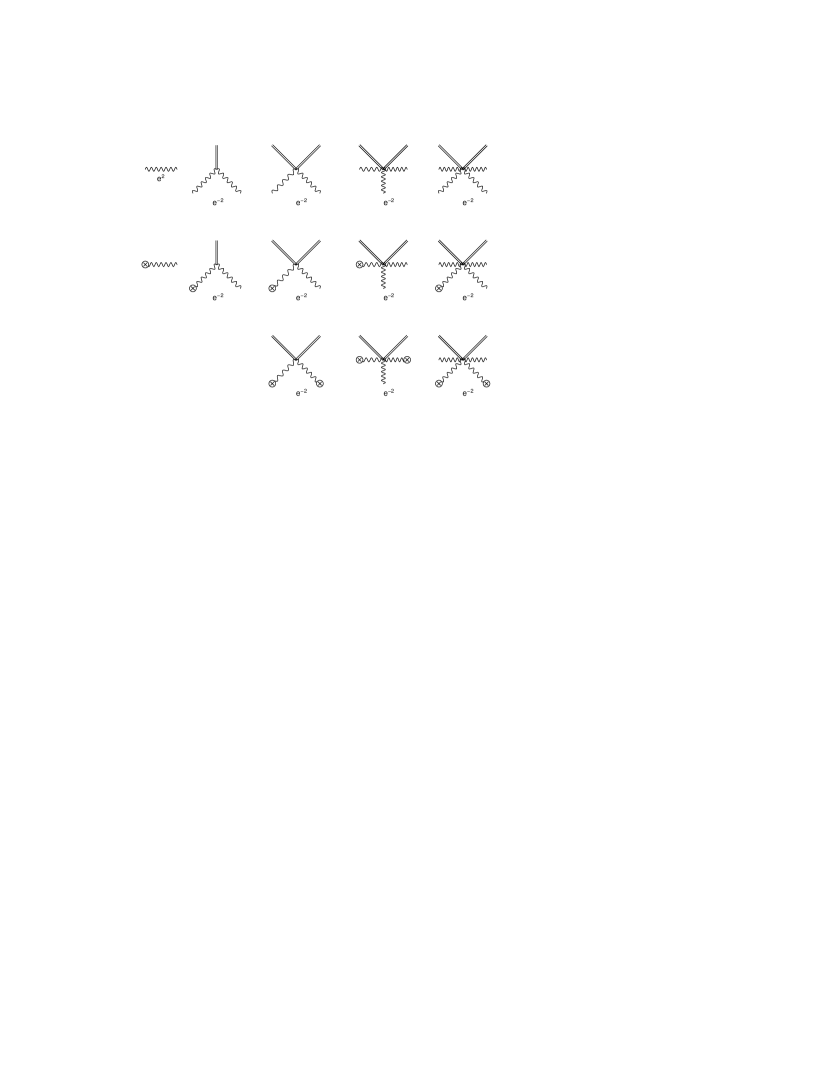
Figure 1: Propagator of gauge field and vertices involving interaction of gauge field (wavy line) with the metric fluctuations (double line). The propagator (first graph) goes like $e^{2}$, while the vertices goes like $1/e^{2}$.

The non-abelian gauge field action is given by,

$$S_{\rm gauge}=-\frac{1}{4e^{2}}\int{\rm d}^{4}x\sqrt{-g}g^{\mu\alpha}g^{\nu\beta}F_{{\mu\nu}}^{a}F_{\alpha\beta}^{a}\,,$$ (2)

where $e$ is the $SU(N)$-gauge coupling, $F_{\mu\nu}^{a}=\partial_{\mu}A_{\nu}^{a}-\partial_{\nu}A_{\mu}^{a}+f^{abc}A_{\mu}^{b}A_{\nu}^{c}$, $A_{\mu}^{a}$ is the gauge vector potential and $f^{abc}$ are the structure constants. Defining quantum theory using the Feynman path-integral for the coupled action of gravity and gauge field given by eq. (1 and 2), we use background field method to do the gauge fixing. In our case where the gravity action is renormalizable and unitary, such a background gauge fixing guarantees a gauge invariant effective action in dimensional regularization scheme thooft2 ; DeWitt1 ; DeWitt2 ; DeWitt3 ; Abbott . The running of gauge coupling constant satisfies the following generic equation,

$$\frac{{\rm d}}{{\rm d}t}\left(\frac{1}{e^{2}}\right)=\frac{a(M^{2}G,\omega,\cdots)}{e^{2}}+b(e^{2},M^{2}G,\omega,\cdots)\,,$$ (3)

where $t=\ln(\mu/\mu_{0})$, the function ‘$a$’ is independent of $e^{2}$ (the gauge coupling), but depends on the other couplings of the action (gravitational and matter sector couplings). It dependence on the gauge group comes implicitly through the dependence of other coupling on the number of generators of the group. The ‘$b$’-term on the other hand depends on all the couplings present in the theory and the gauge group. The ‘dots’ in the definition of ‘$a$’ and ‘$b$’ indicate the dependence on the matter couplings. For small coupling this definition of the beta function is particularly useful as by construction $b$ is a regular function of $e^{2}$ at $e^{2}=0$ in Feynman perturbation theory.

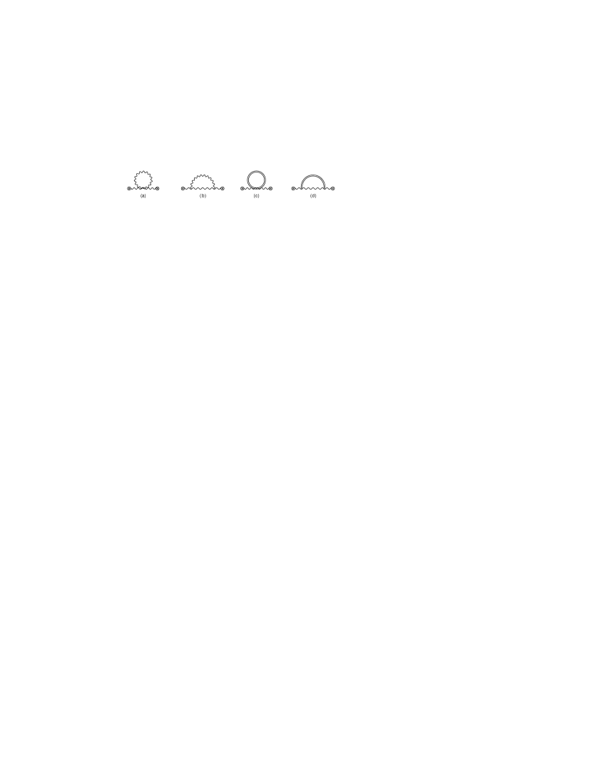
Figure 2: One loop contribution to the running of gauge coupling. The Feynman diagrams (a) and (b) represent the contribution to the running of gauge coupling due to self interaction of the gauge fields (only for non-abelian gauge theories). The diagrams (c) and (d) are one-loop quantum gravity contribution to the gauge coupling (for all gauge theories). Here black dots represent the bare vertices, while wavy lines attached to circle with a cross represent external legs.

From the gauge field action given in eq. (2), we can apply the background field formalism to obtain the propagator of the fluctuating gauge field and the various vertices involving interaction of metric fluctuation with both the background gauge field and the gauge field fluctuation (written in appendix B). As this formalism is explicitly gauge invariant in the background field by construction, therefore the gauge coupling and the wave-function renormalization are the same in this approach. This also means that in this picture one would only have to consider the two-point green function of the background field DeWitt3 ; Abbott . We therefore consider vertices with at most two background gauge field lines. The set of vertices and propagator for the gauge field are depicted in the Fig. 1. Counting the powers of $e^{2}$, it is easy to realize that the propagator for the gauge fluctuation field is proportional to $e^{2}$, while the background gauge field line carries no power of $e^{2}$. All the vertices are proportional to $1/e^{2}$. From the vertices in Fig. 1, we note that any vertex which involve only two gauge field line (either background or fluctuation field) depicts interactions where gravity couples with gauge field purely due to its energy, while any vertex involving more than two gauge field line (either background or fluctuation field) are interaction where there is also charge interactions.

In this formalism at one-loop there are four diagrams that give contribution to the running of gauge coupling: the first two diagrams come because of self interaction between gluons and are only present for non-abelian gauge fields, the other two diagrams give quantum gravity contribution to the running gauge coupling, as shown in Fig. 2. The first two diagrams are only present for non-abelian gauge fields, while the other two diagrams are present for all gauge fields. Studying the $e^{2}$ dependence of the diagrams we notice that both the one-loop diagrams that give quantum gravity contribution to the running of gauge coupling are proportional to $1/e^{2}$, thereby contributing to ‘$a$’ term alone in eq. (3).

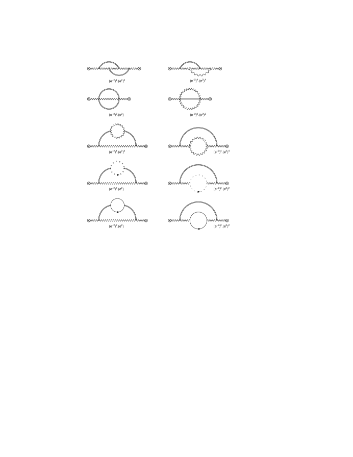
Figure 3: Various Feynman diagrams in the perturbation theory of gauge field coupled with gravity. First column contains diagrams contributing to ‘$a$’-term, while second column contain diagrams contributing to ‘$b$’-term. All diagrams containing 3- or 4-gluon vertex give contributions to ‘$b$’-term of the beta function. Matter loops attached to gluon line contributes to ‘$b$-term, while the one attached to the graviton line contributes to ‘$a$’-term. There are two kinds of ghost: gravitational ghost (which interact with only background and fluctuating metric field) and gauge field ghosts (which interact with background metric, background and fluctuating gauge field line). Gravity ghost contribute to ‘$a$’-term, while gauge field ghost contribute to ‘$b$’-term.

Now we study the nature of ‘$a$’-term to all loops. Here the task is simplified by being in background field formalism where one only has to consider two point correlation function of the background gauge field. We notice that any diagram involving a vertex with three- or four-gluon exchange will only contribute to the ‘$b$’-term of the gauge beta function. This is easily verified by counting the powers of $e^{2}$. For example an inclusion of 3- or 4-gluon vertex in any diagram contributing to the ‘$a$’-term (meaning that it goes like $1/e^{2}$), will result in an increase in the power of $e^{2}$ by at least one factor of $e^{2}$, meaning such diagram will eventually contribute to ‘$b$’-term. This observations can be more clearly checked from the Fig. 3, where appearance of 3- or 4- gluon vertex in a diagram shows that it gives contribution to ‘$b$’-term. So effectively one can ignore these kind of diagrams, this is equivalent to ignoring the three and four gluon terms in the expansion of $F^{a}_{\mu\nu}F^{a{\mu\nu}}$, which is like considering $N^{2}-1$ abelian gauge fields. Diagrams arising from these terms will necessarily contribute to ‘$a$’ term alone, and will be same that is obtained in $U(1)$ gauge field case.

Regarding matter it should be noticed that their interaction with the gauge fields (both background and fluctuation) arise via the kinetic term of the matter fields, where gauge covariant derivative is introduced in order to preserve the gauge invariance of the matter action. Such interaction terms don’t carry any power of $e^{2}$. Matter fields also interact with metric fluctuation. Due to non-linearity of the gravity, such interaction terms are infinite in number. Matter field contribute to the gauge beta function through the loops. When matter field loop is attached to the gauge field line, then it contributes to the ‘$b$’-term, however when it is attached to the internal graviton line, then it contributes to the ‘$a$’-term. For example any diagram contributing to the ‘$a$’-term will still contribute to ‘$a$’-term when matter loop is attached or inserted in a graviton line. This is because vertices involving interaction of matter with graviton don’t carry any power of $e^{2}$. But on other hand when matter loop is inserted/attached to gluon line then the power of $e^{2}$ increase by one. This is because although the new vertices added don’t carry any power of $e^{2}$, but insertion of such loops splits the gluon propagator in two, thereby increasing the power of $e^{2}$ by one. Such modified diagrams will then contribute to ‘$b$’-term. This can be further verified by examining the two-loop graphs given in Fig. 3.

The case of ghost field is a bit different. There are two kind of ghost: gravitational and gauge ghosts. These two ghosts are not independent and mix with each other. This is due to the fact that the gauge field undergoes both deffeomorphism and gauge transformation. This mixing looks problematic but is actually innocuous, as it never contributes to any feynman diagram. This will become more clear later in the section of gauge fixing and ghosts III.1. As a result the gravity and gauge field ghost become independent. Gravity ghosts only interact either with the background metric or with the metric fluctuation field, as a result of which their presence doesn’t alter the power of $e^{2}$ of the diagram. Gauge field ghost on the other hand interacts with the background metric, background gauge field and the gauge fluctuation field. All these interactions don’t carry any powers of $e^{2}$. This means that when ghost loops are inserted in the gauge field line of the diagrams, they tend to increase the power of $e^{2}$ by one. Thus any diagram which was originally contributing to ‘$a$’-term alone, after the inclusion of the gauge field ghost loop will contribute to ‘$b$’-term. This can be further verified by examining the two loop graphs involving the ghost loops depicted in Fig. 3.

These arguments tell that gauge field ghosts when present in the diagrams will always contribute to the ‘$b$’-term of the gauge beta function. On the other hand in the case of matter fields, when the loop is attached to the graviton line then it contributes to ‘$a$’-term, while when it is attached to the gluon line, it contributes to the ‘$b$’-term. Focusing just on the diagrams contributing to ‘$a$’-term alone, is equivalent to considering parts of matter action which doesn’t depend on the gauge field. This is same as saying that one is considering uncharged fields. Thus to sum up, the kind of terms of the total matter action (gauge field action plus the matter action) that contribute to the ‘$a$’-term alone to all loops are: for gauge field action, terms which don’t have 3- or 4-gluon interactions; for the matter action, terms which are independent of the gauge field (same as considering uncharged field). In Fig. 3, although we have demonstrated only up to two loops, but this argument is valid to all loops as discussed in previous paragraphs. However ‘$a$’ term is independent of the gauge coupling $e^{2}$, but can depend upon the gauge group (number of generators of gauge group) via the gravitational and matter couplings dependence on the gauge group. The universality is a manifestation of the fact that the metric fluctuations interact universally to all gauge fields via its energy.

The formal solution of eq. (3) can be written as,

$$\frac{1}{e^{2}}=e^{\int_{0}^{t}a\,{\rm d}t^{\prime}}\biggl{(}\frac{1}{e_{0}^{2}}+\int_{0}^{t}{\rm d}t^{\prime}\,b\,e^{-\int_{0}^{t^{\prime}}a\,{\rm d}t^{\prime\prime}}\biggr{)}$$ (4)

It is evident that for small $e^{2}$ the running of $e^{2}$ depends more dramatically on the sign of $a$. If $a$ is negative then $e^{2}$ diverges as $e^{|a|t}$ for large $t$. If $a$ is positive, then for large $t$, $e^{2}$ vanishes faster than $e^{-|a|t}$ as considered in Robinson ; TomsQuad1 ; TomsQuad2 . If $a=0$, then the standard behavior of the running of gauge coupling qualitatively holds. The above equation is valid to any order in the loop expansion. So the qualitative behavior of $e^{2}$ namely asymptotic freedom can remain unaltered if $a=0$ to all loops. This was examined and studied in NAgauge and found that $a=0$ to all loops off-shell (mistakenly written on-shell, but proof is valid off-shell), while explicitly showing that it is zero at one-loop off-shell (independent of gravity action, regularization scheme and gauge fixing condition). Here we study the coupled system in more detail addressing the ‘$a$’-term to all loops off-shell and will also study the unitarity of the coupled system.

III Effective Action

In this section we study the coupling of higher derivative gravity with gauge field, to compute the quantum gravity correction to the running of gauge couplings. To begin with we consider the path-integral of the coupled gravity and gauge action given in eq. (1 and 2) respectively. This is given by,

$$Z=\int\,{\cal D}\gamma_{\mu\nu}{\cal D}A_{\mu}^{a}\exp\biggl{[}i\biggl{(}S_{\rm GR}+S_{\rm gauge}\biggr{)}\biggr{]}\,,$$ (5)

where $S_{\rm GR}$ is the higher derivative gravity action given in eq. (1), $S_{\rm gauge}$ is the gauge field action given in eq. (2).

We study the deffeomorphism invariant gravity action and gauge invariant gauge field action using background field method DeWitt3 ; Abbott . This has an advantage as by construction it preserves the background gauge field invariance of the effective action. In this formalism the quantum fields of gravity and gauge theory are decomposed into a background and a fluctuation. Keeping the background fixed, the invariance of the fluctuation field of the full action is broken by constraining the fluctuation fields. This procedure results in the generation of certain auxiliary fields called ghosts. The overall resulting action after applying the constraint in the presence of ghost still possess invariance over the background metric and the background gauge field, thereby producing a background gauge invariant effective action.

Writing the quantum metric $\gamma_{\mu\nu}$ as $\bar{g}_{\mu\nu}+h_{\mu\nu}$, where $\bar{g}_{\mu\nu}$ is some arbitrary fixed background and $h_{\mu\nu}$ is the metric fluctuation, we expand the full action in powers of $h_{\mu\nu}$. As the background metric is fixed, therefore the path-integration measure over the quantum metric $\gamma_{\mu\nu}$ gets replaced by the measure over the fluctuation field $h_{\mu\nu}$. Integrating over the fluctuation field $h_{\mu\nu}$ completely also implies that they will only appear as virtual particles inside the loop and never as external legs. Effective action computed after the path-integration over the fluctuation field $h_{\mu\nu}$ being completely deffeomorphism invariant in the background metric, allows one to choose a particular background metric in order to simplify the computation. In particular choosing $\bar{g}_{\mu\nu}=\eta_{\mu\nu}+H_{\mu\nu}$ (while still keeping $H_{\mu\nu}$ generic), allows one to use the methodology and formalism of the flat spacetime quantum field theory. In this way of working it is possible to attribute particle notions to the fields $H_{\mu\nu}$ and $h_{\mu\nu}$, where $h_{\mu\nu}$ will behave as a virtual particle, while $H_{\mu\nu}$ will act as a external particle corresponding to $h_{\mu\nu}$, exactly as is the case in flat spacetime QFT for usual scalar or spinor fields. Attributing particle notions to the fluctuation field $h_{\mu\nu}$ and $H_{\mu\nu}$ allows one to also consider scattering matrix amplitudes. Looking from a different angle it is quickly realized that expanding the gravity action around a flat spacetime and calling the perturbations around it to be $h_{\mu\nu}^{\prime}$, one obtains a highly nonlinear gauge theory in the field $h_{\mu\nu}^{\prime}$. Treating this gauge theory along the lines of background field method, where now the quantum field $h_{\mu\nu}^{\prime}$ is written as $H_{\mu\nu}+h_{\mu\nu}$, allows one to quickly see that this is a flat spacetime QFT with $H_{\mu\nu}$ as an external leg and $h_{\mu\nu}$ as the internal line. Integrating over the fluctuation field $h_{\mu\nu}$, gives one an effective action as a functional of $H_{\mu\nu}$ field, which is the effective action for an arbitrary background expanded about flat spacetime.

In this language one can setup Feynman perturbation theory by expanding the original action of gravity and matter in powers of $h_{\mu\nu}$ and $H_{\mu\nu}$. This series of terms will contain propagator of the $h_{\mu\nu}$ field and various vertices involving interactions of external field $H_{\mu\nu}$ with internal field line $h_{\mu\nu}$. This is the expanded bare action of the theory and carries infinite number of vertices due to nonlinear nature of gravitational field. However, as we still have background gauge invariance, therefore one only needs to do the expansion of the bare action only up to certain finite order in $H_{\mu\nu}$. This means that for studying the behavior of term linear in Ricci scalar curvature under quantum corrections, it is sufficient to expand the bare action up to linear order in $H_{\mu\nu}$, and for studying the behavior of terms quadratic in curvature it is sufficient to expand the bare action up to quadratic in $H_{\mu\nu}$. Such expansion provide all the vertices that will be relevant for study of these kind of terms. This is the privilege of background field method.

For a one-loop computation on the other hand it is sufficient to expand the bare action up to second order in $h_{\mu\nu}$. This although finite in the order of $h_{\mu\nu}$, but is infinite in order of $H_{\mu\nu}$. The restriction on the order of $H_{\mu\nu}$ comes from the requirement of the kind of term that is to be investigated in the effective action. For example probing the issues related to cosmological constant, it is sufficient to put $H_{\mu\nu}=0$ i.e. truncating the series at zeroth order in $H_{\mu\nu}$. Similarly exploring the Ricci scalar term of the effective action demands to consider term up to linear in $H_{\mu\nu}$ and so forth. Investigating quantum gravity contribution to charge renormalization will demand accordingly to consider terms up to zeroth order in $H_{\mu\nu}$, i.e. putting $H_{\mu\nu}=0$.

III.1 Gauge Fixing and Ghosts

The path integration over the gauge and gravitational fields is not well defined. This is due to fact that for certain field configurations the integrand of the functional integral is unity, thereby implying a diverging path integral. This is because gauge and deffeomorphism transformation allows to choose field configurations for which the action is zero. Besides this, the measure of the functional integral over the gauge field is also ill defined, due to over counting of gauge orbits. Both these problems are evaded by constraining both the gauge and metric field thereby breaking the gauge and deffeomorphism invariance of the path integral. This procedure of breaking the invariance of the path integral is echoed by giving rise to ghosts, which is elegantly studied through the methodology of Faddeev-Popov Faddeev .

However, in this style of obtaining the effective action it is difficult to see the invariance, once path integration is performed. This is overcome by using background field method, which explicitly assures the invariance of effective action in the background fields. In this picture the path integral is over the fluctuation fields $h_{\mu\nu}$ and ${\cal A}_{\mu}^{a}$. Gauge fixing of the path integral is done in such a way so that it breaks the invariance over the fluctuation fields, while still preserving the residual invariance over the background fields. In the following we will discuss in detail how the background gauge fixing is done for this coupled system of gauge and gravity fields.

The coupled action of gauge and gravity field being deffeomorphism invariant in the field variables implies, that for an arbitrary vector field $\epsilon^{\rho}$, the action should be invariant under the following transformation of the metric field variable,

$$\delta_{D}\gamma_{\mu\nu}={\cal L}_{\epsilon}\gamma_{\mu\nu}=\epsilon^{\rho}\partial_{\rho}\gamma_{\mu\nu}+\gamma_{\mu\rho}\partial_{\nu}\epsilon^{\rho}+\gamma_{\nu\rho}\partial_{\mu}\epsilon^{\rho}\,,$$ (6)

where ${\cal L}_{\epsilon}\gamma_{\mu\nu}$ is the Lie derivative of the quantum metric $\gamma_{\mu\nu}$ along the vector field $\epsilon^{\rho}$. This metric field when decomposed in to a background ($\bar{g}_{\mu\nu}$) and fluctuation ($h_{\mu\nu}$), allows one to obtain the transformation of the tensor field $h_{\mu\nu}$ while keeping the background fixed. This will imply the following transformation of $h_{\mu\nu}$.

$$\delta_{D}h_{\mu\nu}=\bar{\nabla}_{\mu}\epsilon_{\nu}+\bar{\nabla}_{\nu}\epsilon_{\mu}+\epsilon^{\rho}\bar{\nabla}_{\rho}h_{\mu\nu}+h_{\mu\rho}\bar{\nabla}_{\nu}\epsilon^{\rho}+h_{\nu\rho}\bar{\nabla}_{\mu}\epsilon^{\rho}\,,$$ (7)

where $\bar{\nabla}$ is the covariant derivative whose connection is constructed using the background metric. This is the full transformation of the tensor field $h_{\mu\nu}$. Ignoring terms which are linear in $h_{\mu\nu}$ allows one to investigate only one-loop effects, while they are kept in the complete analysis involving higher-loop studies.

The gauge field action given in eq. (2) on the other hand has two kind of invariances: deffeomorphism invariance and local gauge invariance. For an arbitrary vector field $\epsilon^{\rho}$ and a color vector field $\lambda^{a}$, gauge field action is invariant under the following transformation of the gauge field $A_{\mu}^{a}$.

$${\rm Diff:}\,\,\Rightarrow\,\, \delta_{D}A_{\mu}^{a}={\cal L}_{\epsilon}A_{\mu}^{a}=\epsilon^{\rho}\partial_{\rho}A_{\mu}^{a}+A^{a}_{\rho}\partial_{\mu}\epsilon^{\rho}\,,$$

$${\rm Gauge:}\,\,\Rightarrow\,\, \delta_{g}A_{\mu}^{a}=\partial_{\mu}\lambda^{a}-f^{abc}\lambda^{b}A_{\mu}^{c}\,.$$ (8)

Decomposing the gauge field in to a background $\bar{A}_{\mu}^{a}$ and a fluctuation ${\cal A}_{\mu}^{a}$, implies the following transformation of the fluctuating field ${\cal A}_{\mu}^{a}$ while keeping the background fixed.

$$\delta{\cal A}_{\mu}^{a}=\epsilon^{\rho}\bar{\nabla}_{\rho}\bar{A}_{\mu}^{a}+\bar{A}_{\rho}^{a}\bar{\nabla}_{\mu}\epsilon^{\rho}+\epsilon^{\rho}\bar{\nabla}_{\rho}{\cal A}_{\mu}^{a}+{\cal A}_{\rho}^{a}\bar{\nabla}_{\mu}\epsilon^{\rho}+\bar{\nabla}_{\mu}\lambda^{a}+f^{abc}\bar{A}_{\mu}^{b}\lambda^{c}+f^{abc}{\cal A}_{\mu}^{a}\lambda^{c}\,,$$ (9)

where the first four terms on the rhs of the equality denote the transformation of the fluctuation field ${\cal A}_{\mu}^{a}$ under the deffeomorphism, while the last three terms denote the transformation under the $SU(N)$ gauge group (for abelian gauge fields, the terms proportional to structure constants will be absent). This is the complete transformation of the fluctuation field ${\cal A}_{\mu}^{a}$, under which the gauge field action will be invariant. This invariance of the action under the transformation of the fluctuation field is broken by choosing an appropriate gauge fixing condition for breaking the deffoemorphism and gauge invariance of the action. Choosing a gauge fixing action which is invariant under the background gauge transformation but breaks the invariance under the transformation of the fluctuation field, further assures the preservation of background gauge invariance of the effective action.

The gauge fixing action chosen for fixing the invariance under the transformation of the metric fluctuation field is given by,

$$S^{\rm gravity}_{GF}=\frac{1}{32\pi G\alpha}\int{\rm d}^{d}x\sqrt{-\bar{g}}\biggl{(}\bar{\nabla}^{\rho}h_{\rho\mu}-\frac{1+\rho}{d}\bar{\nabla}_{\mu}h\biggr{)}\,Y^{\mu\nu}\,\biggl{(}\bar{\nabla}^{\sigma}h_{\sigma\nu}-\frac{1+\rho}{d}\bar{\nabla}_{\nu}h\biggr{)}\,.$$ (10)

where $\alpha$ and $\rho$ are gauge parameters, while $Y_{\mu\nu}$ is either a constant or some differential operator depending upon the gravity theory under consideration. In the case of higher-derivative gravity like the one described by action in eq. (1), we consider higher-derivative type gauge fixing by taking $Y_{\mu\nu}=(-\bar{g}_{\mu\nu}\bar{\Box}+\beta\bar{\nabla}_{\mu}\bar{\nabla}_{\nu})$, where $\Box=\bar{\nabla}_{\mu}\bar{\nabla}^{\mu}$. Similarly the fluctuating gauge field is constrained by choosing the following gauge fixing action,

$$S^{\rm gauge}_{GF}=\frac{1}{2\xi}\left(-\frac{1}{e^{2}}\right)\int{\rm d}^{d}x\sqrt{-\bar{g}}\left(\textbf{D}_{\mu}\mathcal{A}^{a\mu}\right)^{2}\,,$$ (11)

where $\xi$ is a gauge parameter. Here D is the covariant derivative constructed with background metric and the background gauge field. Its action on the fluctuation gauge field is given by,

$$\textbf{D}_{\mu}{\cal A}_{\nu}^{a}=\partial_{\mu}{\cal A}_{\nu}^{a}-\bar{\Gamma}_{\mu}{}^{\alpha}{}_{\nu}{\cal A}_{\alpha}^{a}+f^{abc}\bar{A}_{\mu}^{b}{\cal A}_{\nu}^{c}\,.$$ (12)

The ghost action for these gauge fixing conditions can be obtained by using the Faddeev-Popov trick Faddeev . Calling in general the gauge fixing condition for gravitational field $h_{\mu\nu}$ to be $F_{1\mu}=0$, while the gauge fixing condition for the fluctuating gauge field ${\cal A}_{\mu}^{a}$ to be $F_{2}^{a}=0$ (in the present case we have $F_{1\mu}=\bar{\nabla}^{\rho}h_{\rho\mu}-\frac{1+\rho}{d}\bar{\nabla}_{\mu}h$ and $F_{2}^{a}=\textbf{D}_{\mu}\mathcal{A}^{a\mu}$), we introduce them in the path integral of the fluctuating fields by multiplying it with unity in the following form.

$$1=\int{\cal D}F^{\epsilon\lambda}_{1\mu}{\cal D}F_{2}^{a\epsilon\lambda}\left(\det Y\right)^{\frac{1}{2}}\exp\biggl{[}\frac{i}{32\pi G\alpha}\int{\rm d}^{d}x\sqrt{-\bar{g}}F^{\epsilon\lambda}_{1\mu}Y^{\mu\nu}F^{\epsilon\lambda}_{1\nu}+\frac{i}{2\xi e^{2}}\int{\rm d}^{d}x\sqrt{-\bar{g}}F_{2}^{a\epsilon\lambda}F^{\epsilon\lambda}_{2a}\biggr{]}\,,$$ (13)

where $F_{1\mu}^{\epsilon\lambda}$ and $F_{2}^{a\epsilon\lambda}$ are the gauge transformed $F_{1\mu}$ and $F_{2}^{a}$ respectively. If $Y^{\mu\nu}$ did not contain any derivatives, then this determinant would be trivial, however it will not be so if $Y^{\mu\nu}$ contains derivative operators, which is the case in higher-derivative gravity. The original path integral (without gauge fixing) being invariant under transformation eq. (7 and 9) of the fluctuation fields $h_{\mu\nu}$ and ${\cal A}_{\mu}^{a}$, implies that the integration variable $h_{\mu\nu}$ and ${\cal A}_{\mu}^{a}$ can be changed to transformed fields $h_{\mu\nu}^{\epsilon}$ and ${\cal A}_{\mu}^{a\epsilon\lambda}$. This transformation don’t give rise to any non-trivial jacobians in the path-integral measure of the gauge and gravity field. Writing the measure over $F^{\epsilon\lambda}_{1\mu}$ and $F_{2}^{a\epsilon\lambda}$, as measure over the transformation variables $\epsilon^{\rho}$ and $\lambda^{a}$, introduces a non-trivial jacobian in the path integral. This is the Faddeev-Popov determinant and is worked out as follows.

$$dF_{1\mu}^{\epsilon\lambda}=\frac{\partial F_{1\mu}}{\partial\epsilon^{\rho}}d\epsilon^{\rho}+\frac{\partial F_{1\mu}}{\partial\lambda^{b}}d\lambda^{b}\,,$$

$$dF_{2}^{a\epsilon\lambda}=\frac{\partial F_{2}^{a}}{\partial\epsilon^{\rho}}d\epsilon^{\rho}+\frac{\partial F_{2}^{a}}{\partial\lambda^{b}}d\lambda^{b}\,.$$ (14)

This means that the measure ${\cal D}F_{1\mu}^{\epsilon\lambda}{\cal D}F_{2}^{a\epsilon\lambda}$ transforms as,

$${\cal D}F_{1\mu}^{\epsilon\lambda}{\cal D}F_{2}^{a\epsilon\lambda}=\det\left(\large\begin{array}[]{c c}\frac{\partial F_{1\mu}}{\partial\epsilon^{\rho}}&\frac{\partial F_{1\mu}}{\partial\lambda^{b}}\\ &\\ \frac{\partial F_{2}^{a}}{\partial\epsilon^{\rho}}&\frac{\partial F_{2}^{a}}{\partial\lambda^{b}}\end{array}\right){\cal D}\epsilon^{\rho}{\cal D}\lambda^{b}\,.$$ (15)

In the background field formalism, this jacobian consist of background covariant derivative, background and fluctuation fields. As the determinant is independent of the transformation parameters $\epsilon^{\rho}$ and $\lambda^{a}$, therefore it can be taken out of the functional integral over $\epsilon^{\rho}$ and $\lambda^{a}$. Changing the integration variable from $h_{\mu\nu}^{\epsilon}$ and ${\cal A}_{\mu}^{a\epsilon\lambda}$ to $h_{\mu\nu}$ and ${\cal A}_{\mu}^{a}$ respectively, and ignoring the infinite constant generated by integrating over $\epsilon^{\rho}$ and $\lambda^{a}$, gives us the gauge fixed path integral including the determinants.

These functional determinants can be exponentiated by making use of appropriate auxiliary fields. Writing the functional determinant $(\det Y)^{1/2}$ as a product of two determinants $(\det\,Y)\times(\det\,Y)^{-1/2}$, allows us to combine the former with the Faddeev-Popov determinant in eq. (15), which is then exponentiated by making use of anti-commuting auxiliary fields, while the later determinant $(\det\,Y)^{-1/2}$ is exponentiated by making use of commuting auxiliary fields. The former auxiliary fields are known as Feddeev-Popov ghosts, while the auxiliary field in the later case is known as Neilsen-Kallosh ghosts Kallosh ; Nielsen . The path integral of the full ghost sector is given by,

$$\int{\cal D}\bar{C}_{\mu}{\cal D}C_{\nu}{\cal D}\bar{c}^{a}{\cal D}c^{b}{\cal D}\theta_{\alpha}\,\,\exp\biggl{[}-i\int{\rm d}^{d}x\sqrt{-\bar{g}}\,\left(\begin{array}[]{c c}\bar{C}_{\mu}&\bar{c}^{a}\end{array}\right)\cdot$$ (17)

$$\left(\begin{array}[]{c c}Y^{\mu\nu}\,\partial F_{1\nu}/\partial\epsilon^{\rho}&Y^{\mu\nu}\partial F_{1\nu}/\partial\lambda^{b}\\ &\\ \partial F_{2}^{a}/\partial\epsilon^{\rho}&\partial F_{2}^{a}/\partial\lambda^{b}\end{array}\right)\cdot\left(\begin{array}[]{c}C^{\rho}\\ c^{b}\end{array}\right)-\frac{i}{2}\int{\rm d}^{d}x\sqrt{-\bar{g}}\,\theta_{\alpha}Y^{\alpha\beta}\theta_{\beta}\biggr{]}\,,$$ (23)

where $\bar{C}_{\mu}$ and $C_{\nu}$ are anti-commuting fields arising from the gauge fixing in the gravitational sector, while $\bar{c}^{a}$ and $c^{b}$ are anti-commuting fields arising from the gauge fixing in the gauge field sector and $\theta_{\mu}$ is the commuting ghost arising due to fact that $Y_{\mu\nu}$ contains derivatives. It is crucial to note here that in the coupled system of gauge field with gravity, there will always be mixing between the gravitational and gauge ghosts. The mixing term $Y^{\mu\nu}\partial F_{1\nu}/\partial\lambda^{b}$ will arise, if we choose a gauge fixing condition for the gravitational field $h_{\mu\nu}$ such that it also contain terms involving gauge fluctuation field ${\cal A}_{\mu}^{a}$. In the absence of such term, this mixing term will be always zero. However, the mixing term $\partial F_{2}^{a}/\partial\epsilon^{\rho}$ will be always non-zero, as the gauge fluctuation field ${\cal A}_{\mu}^{a}$ undergoes both deffeomorphism and gauge transformation.

In the case when $F_{1\mu}$ and $F_{2}^{a}$ are given as in eq. (10) and (11) respectively, the Faddev-Popov ghost action is given by,

$$S^{FP}_{\rm gh}=-\int{\rm d}^{d}x\sqrt{-\bar{g}}\biggl{[}\bar{C}_{\mu}X^{\mu}_{1\rho}C^{\rho}+\bar{c}^{a}X^{a}_{2\rho}C^{\rho}+\bar{c}^{a}X_{3}^{ab}c^{b}\,,\biggr{]}\,,$$ (24)

where,

$$X^{\mu}_{1\rho} = (\bar{g}^{\mu\nu}\bar{\Box}+\beta\bar{\nabla}^{\mu}\bar{\nabla}^{\nu})\biggl{[}\bar{\nabla}_{\rho}\bar{\nabla}_{\nu}+\bar{g}_{\nu\rho}\Box-\frac{2(1+\rho)}{d}\bar{\nabla}_{\nu}\bar{\nabla}_{\rho}+\bar{\nabla}_{\rho}h_{\sigma\nu}\bar{\nabla}^{\sigma}+\bar{\nabla}^{\sigma}\bar{\nabla}_{\rho}h_{\sigma\nu}$$ (25)

$$+\bar{\nabla}^{\sigma}h_{\nu\rho}\bar{\nabla}_{\sigma}+h_{\nu\rho}\bar{\Box}+\bar{\nabla}^{\sigma}h_{\sigma\rho}\bar{\nabla}_{\nu}+h_{\sigma\rho}\bar{\nabla}^{\sigma}\bar{\nabla}_{\nu}$$

$$-\frac{1+\rho}{d}\biggl{(}\bar{\nabla}_{\rho}h\bar{\nabla}_{\nu}+\bar{\nabla}_{\nu}\bar{\nabla}_{\rho}h+2\bar{\nabla}_{\nu}h_{\sigma\rho}\bar{\nabla}^{\sigma}+2h_{\sigma\rho}\bar{\nabla}_{\nu}\bar{\nabla}^{\sigma}\biggr{)}\biggr{]}\,,$$

$$X^{a}_{2\rho} = \bar{\nabla}_{\rho}\bar{A}_{\sigma}^{a}\bar{\nabla}^{\sigma}+\bar{\nabla}^{\sigma}\bar{\nabla}_{\rho}\bar{A}_{\sigma}^{a}+\bar{\nabla}^{\sigma}\bar{A}_{\rho}^{a}\bar{\nabla}_{\sigma}+\bar{A}^{a}\rho\bar{\Box}+\bar{\nabla}_{\rho}{\cal A}^{a}_{\sigma}\bar{\nabla}^{\sigma}+\bar{\nabla}_{\sigma}\bar{\nabla}_{\rho}{\cal A}^{a\sigma}+\bar{\nabla}^{\sigma}{\cal A}^{a}_{\rho}\bar{\nabla}_{\sigma}$$ (26)

$$+{\cal A}^{a}_{\rho}\bar{\Box}+f^{abc}\bar{A}^{b\sigma}\bar{\nabla}\bar{A}^{c}_{\sigma}+f^{abc}\bar{A}^{b\sigma}\bar{A}^{c}_{\rho}\bar{\nabla}_{\sigma}+f^{abc}\bar{A}^{b\sigma}\bar{\nabla}_{\rho}{\cal A}^{c}_{\sigma}+f^{abc}\bar{A}^{b\sigma}{\cal A}^{c}_{\rho}\bar{\nabla}_{\sigma}\,,$$

$$X_{3}^{ab} = \delta^{ab}\bar{\Box}-f^{abc}\bar{\nabla}^{\sigma}\bar{A}^{c}_{\sigma}-2f^{abc}\bar{A}^{c}_{\sigma}\bar{\nabla}^{\sigma}-f^{abc}\bar{\nabla}^{\sigma}{\cal A}^{c}_{\sigma}-f^{abc}{\cal A}^{c}_{\sigma}\bar{\nabla}^{\sigma}$$ (27)

$$+f^{aec}f^{cdb}\bar{A}^{e\sigma}\bar{A}^{d}_{\sigma}+f^{aec}f^{cdb}\bar{A}^{e\sigma}{\cal A}^{d}_{\sigma}\,.$$

It should be noted that for the kind of gauge fixing condition considered here in eq. (10) and (11), only the mixing term $\partial F_{2}^{a}/\partial\epsilon^{\rho}$ is non-zero, while the other mixing term $Y^{\mu\nu}\partial F_{1\nu}/\partial\lambda^{b}$ is zero. This means that there is no interaction between gravitational ghost $\bar{C}_{\mu}$ and gauge ghost $c^{a}$. This has an important consequence. This will imply that in this kind of gauge fixing, there will not be any closed loop Feynman diagram with one line in the loop to be gravitational ghost, while the other gauge ghost. Therefore, the presence of mixing term becomes completely innocuous. Had the other mixing term in the Faddeev-Popov determinant $Y^{\mu\nu}\partial F_{1\nu}/\partial\lambda^{b}$ been nonzero, then we will have interaction term in the ghost action involving $\bar{C}_{\mu}$ and $c^{a}$. In such cases there will graphs involving loop with one gravitational ghost and one gauge ghost.

III.2 Gravitational Field Propagator

The propagator of the fluctuating quantum field $h_{\mu\nu}$ is given is obtained by expanding the bare gravitational action eq. (1) up to second order in $h_{\mu\nu}$ around flat spacetime background. This is given by,

$$\delta^{2}S_{\rm GR}=\int\frac{{\rm d}^{d}x}{32\pi G}\biggl{[}-h\partial_{\mu}\partial_{\nu}h^{\mu\nu}+\frac{1}{2}h\Box h-\partial_{\nu}h^{\mu\nu}\partial_{\rho}h^{\rho}_{\mu}-\frac{1}{2}h_{\mu\nu}\Box h^{\mu\nu}$$

$$-\frac{1}{2M^{2}}(\partial_{\rho}\partial_{\nu}h^{\rho}_{\mu}+\partial_{\rho}\partial_{\mu}h^{\rho}_{\nu}-\partial_{\mu}\partial_{\nu}h-\Box h_{\mu\nu})(\partial^{\sigma}\partial^{\nu}h_{\sigma}^{\mu}+\partial^{\sigma}\partial^{\mu}h_{\sigma}^{\nu}-\partial^{\mu}\partial^{\nu}h-\Box h^{{\mu\nu}})$$

$$+\frac{2}{M^{2}}\frac{d+(d-2)\omega}{4d(d-1)}(\partial_{\mu}\partial_{\nu}h^{\mu\nu}-\Box h)(\partial_{\alpha}\partial_{\beta}h^{\alpha\beta}-\Box h)\biggr{]}\,.$$ (28)

By making use of the complete set of orthogonal projectors in flat space for the symmetric rank-2 tensor field (see appendix A), this can be re-written in momentum space in term of projectors,

$$\delta^{2}S_{\rm GR}=\frac{1}{32\pi G}\int\frac{{\rm d}^{d}q}{(2\pi)^{d}}h_{{\mu\nu}}\biggl{[}-\frac{q^{2}}{2M^{2}}(q^{2}-M^{2})P_{2}^{{\mu\nu}\rho\sigma}+\frac{(d-2)\omega}{2M^{2}}q^{2}\left(q^{2}-\frac{M^{2}}{\omega}\right)P_{s}^{{\mu\nu}\rho\sigma}\biggr{]}h_{\rho\sigma}\,.$$ (29)

The gauge fixing action eq. (10), with flat spacetime as the background can also be written in the language of projectors as follows,

$$S_{\rm GF}=\frac{1}{32\pi G\alpha}\int\frac{{\rm d}^{d}q}{(2\pi)^{d}}h_{{\mu\nu}}\,q^{4}\,\biggl{[}-\frac{1}{2}P_{1}^{{\mu\nu}\rho\sigma}+\frac{1-\beta}{d^{2}}\biggl{\{}(1+\rho)^{2}(d-1)P_{s}^{{\mu\nu}\rho\sigma}$$

$$+(d-1-\rho)^{2}P_{w}^{{\mu\nu}\rho\sigma}-\sqrt{d-1}(1+\rho)(d-1-\rho)\left(P_{sw}^{{\mu\nu}\rho\sigma}+P_{ws}^{{\mu\nu}\rho\sigma}\right)\biggr{\}}\biggr{]}h_{\rho\sigma}\,.$$ (30)

Writing the gauge fixing action in terms of projectors is advantageous. It shows that it only give contribution to the longitudinal modes of the field, and not to the transverse spin-2 projector. This is expected as the spin-2 component is gauge invariant under the diffeomorphism transformation of the fluctuation field $h_{\mu\nu}$. Also it should be noticed that the components corresponding to each of the projector is of $q^{4}$ type. This is due to fact that $Y_{\mu\nu}$ contains derivatives. Had we chosen $Y_{\mu\nu}$ to be proportional to constant, then we would have got coefficients corresponding to each of projector in gauge fixing action to be of $q^{2}$ type.

When gauge parameters take arbitrary values then this will over fix the gauge redundancies, and there will be longitudinal terms in the gravity propagator. Such terms may not give any contribution to one-loop diagrams (except for quadratic divergent ones) but at higher loops, contribution from them is unavoidable. However the $S$-matrix constructed will be gauge-invariant. Its only in Landau gauge ($\rho=-1$, $\beta=0$ and $\alpha=0$) that we don’t have any longitudinal modes in the propagator (and don’t have to worry about ghosts) describing physical degrees of freedom correctly. The gravity propagator in this gauge is given by,

$$D^{{\mu\nu}\rho\sigma}=(16\pi G)\biggl{[}-\frac{2M^{2}P_{2}^{{\mu\nu}\rho\sigma}}{q^{2}(q^{2}-M^{2})}+\frac{2M^{2}}{(d-2)\omega}\frac{P_{s}^{{\mu\nu}\rho\sigma}}{q^{2}(q^{2}-M^{2}/\omega)}\biggr{]}=(\Delta_{G}^{-1})^{{\mu\nu}\rho\sigma}\,,$$ (31)

where $\Delta_{G}^{{\mu\nu}\alpha\beta}$ is the inverse propagator for the $h_{\mu\nu}$ field including the gauge fixing and is symmetric in ${\mu\nu}$ and $\alpha\beta$. In co-ordinate space this can be written as,

$$\frac{1}{2}\int\,{\rm d}^{d}x\,h_{\mu\nu}\,\Delta_{G}^{{\mu\nu}\alpha\beta}h_{\alpha\beta}\,.$$ (32)

The graviton propagator written in eq. (31) can be analyzed further by doing partial fraction decomposition. This enumerates the various propagating modes of the theory. This is given by,

$$D^{{\mu\nu},\alpha\beta}=16\pi G\cdot\Biggl{[}\frac{(2P_{2}-(2/(d-2))P_{s})^{\mu\nu,\alpha\beta}}{q^{2}+i\,\epsilon}+\frac{2}{d-2}\frac{(P_{s})^{\mu\nu,\alpha\beta}}{q^{2}-M^{2}/\omega+i\epsilon}-\frac{2\,(P_{2})^{\mu\nu,\alpha\beta}}{q^{2}-M^{2}+i\epsilon}\Biggr{]}\,.$$ (33)

We note that the first term is the usual massless graviton with two degrees of freedom, the second term is a massive scalar with mass $M/\sqrt{\omega}$ and has one degree of freedom (we call it ‘Riccion’), while the third term is a massive spin-2 mode of mass $M$ with five degrees of freedom (we call it $M$-mode). This mode has negative residue and breaks unitarity at tree level. However when quantum corrections are taken into account, it is shown that the mass of this mode runs in such a way so that it is always above the running energy scale NarainA1 ; NarainA2 .

Having obtained the propagator for the gravitational field, we move on to study the gauge field action and its coupling with the gravitational field $h_{\mu\nu}$. In the next subsection we will build up the formalism to compute the quantum gravity contribution to the gauge field action.

III.3 Formalism

Under the decomposition of gauge field in to background and fluctuation as $A_{\mu}^{a}=\bar{A}_{\mu}^{a}+{\cal A}_{\mu}^{a}$, the expansion of field strength tensor $F_{\mu\nu}^{a}$ is given by, $F_{\mu\nu}^{a}=\bar{F}_{\mu\nu}^{a}+D_{\mu}\mathcal{A}_{\nu}^{a}-D_{\nu}\mathcal{A}_{\mu}^{a}+f^{abc}\mathcal{A}_{\mu}^{b}\mathcal{A}_{\nu}^{c}$, where $\bar{F}_{\mu\nu}^{a}=\partial_{\mu}\bar{A}_{\nu}^{a}-\partial_{\nu}\bar{A}_{\mu}^{a}+f^{abc}\bar{A}_{\mu}^{b}\bar{A}_{\nu}^{c}$ and $D_{\mu}\mathcal{A}_{\nu}=\partial_{\mu}\mathcal{A}_{\nu}^{a}+f^{abc}\bar{A}_{\mu}^{b}\mathcal{A}_{\nu}^{c}$.

To compute the one-loop quantum gravity contribution to the running of gauge coupling, it is sufficient to expand the gauge field action up to quadratic in $h_{\mu\nu}$ and $\mathcal{A}^{a}_{\mu}$ around the flat metric. This will give rise to various vertices that will be relevant for the one-loop computation and the gauge field propagator. This second variation is given by,

$$\delta^{2}S_{\rm gauge}=-\int\frac{{\rm d}^{4}x\sqrt{-g}}{8e^{2}}\Biggl{[}\biggl{\{}\left(\frac{1}{4}h^{2}-\frac{1}{2}h_{\mu\nu}h^{\mu\nu}\right)g^{\mu\alpha}g^{\nu\beta}-2hh^{\mu\alpha}g^{\nu\beta}+4h^{\mu\rho}h_{\rho}{}^{\alpha}g^{\nu\beta}$$

$$+2h^{\mu\alpha}h^{\nu\beta}\biggr{\}}F_{\mu\nu}^{a}F_{\alpha\beta}^{a}+2hg^{\mu\alpha}g^{\nu\beta}\left(D_{\mu}\mathcal{A}_{\nu}^{a}-D_{\nu}\mathcal{A}_{\mu}^{a}\right)F_{\alpha\beta}^{a}-8h^{\mu\alpha}g^{\nu\beta}\left(D_{\mu}\mathcal{A}_{\nu}^{a}-D_{\nu}\mathcal{A}_{\mu}^{a}\right)F_{\alpha\beta}^{a}$$

$$+4g^{\mu\alpha}g^{\nu\beta}f^{abc}\mathcal{A}_{\mu}^{b}\mathcal{A}_{\nu}^{c}F_{\alpha\beta}^{a}+2\eta^{\mu\alpha}\eta^{\nu\beta}\left(D_{\mu}\mathcal{A}_{\nu}^{a}-D_{\nu}\mathcal{A}_{\mu}^{a}\right)\left(D_{\alpha}\mathcal{A}_{\beta}^{a}-D_{\beta}\mathcal{A}_{\alpha}^{a}\right)\Biggr{]}\,.$$ (34)

The gauge fixing action for the gauge field given in eq. (11) is written for arbitrary background metric. This is crucial so as to have diffeomorphism invariance for the effective action obtained by integrating out the quantum fluctuations. However for investigating issues related to charge renormalization (divergent part of the effective action), it is sufficient to consider the flat background. This is justified further by writing the arbitrary background metric $\bar{g}_{\mu\nu}$ as $\eta_{\mu\nu}+H_{\mu\nu}$, and expanding the gauge fixing action in powers of $H_{\mu\nu}$. The leading term of this series is the same as is obtained when background is flat, and is the only relevant term required for studying divergent contributions which are zeroth order in curvature of background metric. This gauge fixing action when added to the second variation of the gauge field action, gives the gauge fixed propagator and the vertices, which have been written in the appendix B.

Having obtained the expansion of the bare action of gravity and gauge field up to second order in fields (which is all that is needed in the one-loop computation), we start by considering the path-integral over the fluctuation fields. The zeroth order term being independent of the fluctuation fields, can be taken out of the path-integral. The linear term can be removed by redefining the fluctuation fields, which only give rise to a trivial Jacobian from the functional measure. The quadratic piece can now be tackled easily by clubbing the two fields to form a multiplet $\Phi=\left(h_{\mu\nu},\mathcal{A}^{a}_{\alpha}\right)$. This allows one to express the second variation in a more compact notation. The residual path-integral along with the source terms has the following form,

$$Z[\textbf{J}]=\exp\biggl{[}i\biggl{(}S_{\rm GR}(\bar{g})+S_{\rm gauge}(\bar{A})\biggr{)}\biggl{]}\int\,{\cal D}\Phi\,\exp\biggl{[}\frac{i}{2}\int\,{\rm d}^{d}x\Phi\cdot\textbf{M}\cdot\Phi^{T}+i\Phi\cdot\textbf{J}^{T}\biggr{]}\,,$$ (35)

where $\textbf{J}=\{t_{\mu\nu},U_{\mu}^{a}\}$ is the source multiplet which couples with the fluctuation fields $\Phi=\left(h_{\mu\nu},\mathcal{A}^{a}_{\alpha}\right)$, and

$$\frac{1}{2}\int{\rm d}^{d}x\,\Phi\cdot\textbf{M}\cdot\Phi^{T}=\frac{1}{2}\int{\rm d}^{d}x\,\left(\begin{array}[]{c c}h_{\mu\nu}&\mathcal{A}^{a}_{\gamma^{\prime}}\end{array}\right)\cdot\textbf{M}\cdot\left(\begin{array}[]{c}h_{\rho\sigma}\\ \mathcal{A}^{c}_{\gamma}\end{array}\right)$$ (39)

$$\textbf{M}=\biggl{[}\begin{array}[]{c c}\Delta_{G}^{\mu\nu\rho\sigma}-\frac{1}{4e^{2}}V^{\mu\nu\rho\sigma}_{\theta\tau\alpha\beta}\,\bar{F}^{a\theta\tau}\,\bar{F}^{a\alpha\beta}&-\frac{2}{4e^{2}}V^{c\mu\nu\gamma^{\prime}\gamma}D_{\gamma^{\prime}}\\ \frac{2}{4e^{2}}V^{a\rho\sigma\gamma\gamma^{\prime}}D_{\gamma}+\frac{2}{4e^{2}}D_{\gamma}V^{a\rho\sigma\gamma\gamma^{\prime}}&-\frac{1}{4e^{2}}\left(\Delta_{g}+\Delta_{1}+\Delta_{2}+\Delta_{3}\right)^{ac\gamma^{\prime}\gamma}\end{array}\biggr{]}\,.$$ (42)

From the generating functional $Z$ we define the one-particle-irreducible (1PI) generating functional $\Gamma=W[\textbf{J}]-\int\,{\rm d}^{d}x\textbf{J}\cdot\langle\Phi^{T}\rangle$, where $W[\textbf{J}]=-i\ln Z[\textbf{J}]$ and $\langle\Phi^{T}\rangle$ is the expectation value of $\Phi^{T}$ field. The 1PI generating functional $\Gamma$ is also the effective action. Performing the $\Phi$ integration one obtains,

$$\exp\biggl{[}i\biggl{(}\Gamma+\int\,{\rm d}^{d}x\textbf{J}\cdot\langle\Phi^{T}\rangle\biggr{)}\biggr{]}=\exp\biggl{[}i\biggl{(}S_{\rm GR}(\bar{g})+S_{\rm gauge}(\bar{A})-\frac{1}{4}\int\,{\rm d}^{d}x\textbf{J}\cdot\textbf{M}^{-1}\cdot\textbf{J}^{T}\biggr{)}\biggr{]}\cdot\biggl{(}\det\,\textbf{M}\biggr{)}^{-1/2}$$ (43)

For zero source, the above equation gives the expression for 1-loop effective action $\Gamma$,

$$\Gamma^{\rm 1-loop}[\Phi]=S_{\rm GR}(\bar{g})+S_{\rm gauge}(\bar{A})+\frac{i}{2}{\rm Tr}\ln\textbf{M}\,,$$ (44)

where the first two terms correspond to tree level diagrams, while the last term contains 1-loop quantum corrections. Our task in the following is to compute the divergent terms present in ${\rm Tr}\ln\textbf{M}$ which are proportional to $\int\,{\rm d}^{d}xF_{\mu\nu}^{a}F^{a{\mu\nu}}$. There are several ways of obtaining it, but here we will do it by expanding the $\ln\textbf{M}$ in a power series, and studying terms which will contain divergent contribution proportional to $\int\,{\rm d}^{d}xF_{\mu\nu}^{a}F^{a{\mu\nu}}$. In our case writing $\textbf{M}=\Delta+\textbf{V}$ (where the first term contains only the propagator of the theory and the second terms contains the interactions), we have,

$$\textbf{M}=\biggl{[}\begin{array}[]{c c}\Delta_{G}^{{\mu\nu}\rho\sigma}&0\\ 0&-\frac{1}{4e^{2}}\Delta_{g}^{ac\gamma^{\prime}\gamma}\end{array}\biggr{]}-\frac{1}{4e^{2}}\biggl{[}\begin{array}[]{c c}V^{{\mu\nu}\rho\sigma}_{\theta\tau\alpha\beta}\bar{F}^{a\theta\tau}\bar{F}^{a\alpha\beta}&2V^{c{\mu\nu}\gamma^{\prime}\gamma}D_{\gamma^{\prime}}\\ -2V^{a\rho\sigma\gamma\gamma^{\prime}}D_{\gamma}-2D_{\gamma}V^{\rho\sigma\gamma\gamma^{\prime}}&\left(\Delta_{1}+\Delta_{2}+\Delta_{3}\right)^{ac\gamma^{\prime}\gamma}\end{array}\biggr{]}\,,$$ (45)

$\Delta$ can be pulled outside so that the logarithm of the residual expression $\left(\textbf{I}+\Delta^{-1}\cdot\textbf{V}\right)$ (where I is the identity in field space), can be easily expanded as power series in $\Delta^{-1}\cdot\textbf{V}$.

$${\rm Tr}\ln\textbf{M}={\rm Tr}\ln\Delta\cdot\biggl{(}\textbf{I}+\Delta^{-1}\cdot\textbf{V}\biggr{)}={\rm Tr}\ln\Delta+{\rm Tr}\biggl{[}\Delta^{-1}\cdot\textbf{V}-\frac{1}{2}\Delta^{-1}\cdot\textbf{V}\cdot\Delta^{-1}\cdot\textbf{V}+\cdots\biggr{]}\,.$$ (46)

After pulling out $\Delta$, ${\bf M}$ has the following expression in index form,

$$\textbf{M}=\biggl{(}\begin{array}[]{c c}\Delta_{G}^{\mu^{\prime}\nu^{\prime},{\mu\nu}}&0\\ 0&-\frac{1}{4e^{2}}\Delta_{g}^{a^{\prime}a\gamma^{\prime}\kappa}\end{array}\biggr{)}\cdot\Biggl{[}\biggl{(}\begin{array}[]{c c}\bf{I}^{\rho\sigma}_{{\mu\nu}}&0\\ 0&\delta^{c}_{a}\delta^{\gamma}_{\kappa}\end{array}\biggr{)}$$ (51)

$$-\frac{1}{4e^{2}}\biggl{(}\begin{array}[]{c c}\left(\Delta_{G}^{-1}\right)_{{\mu\nu}}{}^{\alpha^{\prime}\beta^{\prime}}V_{\alpha^{\prime}\beta^{\prime}}{}^{\rho\sigma}{}_{\theta\tau\alpha\beta}\bar{F}^{b\theta\tau}\bar{F}^{b\alpha\beta}&2\left(\Delta_{G}^{-1}\right)_{{\mu\nu}}{}^{\alpha^{\prime}\beta^{\prime}}V^{c}{}_{\alpha^{\prime}\beta^{\prime}}{}^{\gamma^{\prime}\gamma}D_{\gamma^{\prime}}\\ 8e^{2}\left(\Delta_{g}^{-1}\right)_{a\kappa}^{b\tau}\left(V_{b}{}^{\rho\sigma\gamma}{}_{\tau}D_{\gamma}+D_{\gamma}V_{b}{}^{\rho\sigma\gamma}{}_{\tau}\right)&-4e^{2}\left(\Delta_{g}^{-1}\right)_{a\kappa}^{b\tau}\left(\Delta_{1}+\Delta_{2}+\Delta_{3}\right)_{b}{}^{c}{}_{\tau}{}^{\gamma}\end{array}\biggr{)}\Biggr{]}$$ (54)

In the present case we have taken the background metric to be flat, therefore one can ignore the contribution coming from first term in the expansion in eq. (46), which gives just a normalization constant. But had we had an arbitrary background which has a nonzero curvature, then this term cannot be ignored and actually give contribution which goes in renormalizing the gravitational parameters.

In the following we will compute the one-loop quantum gravity corrections to the running of gauge coupling, by evaluating the various terms of the series in eq. (46).

III.4 Graphs

We note that the series given in eq. (46) contains various 1-loop diagrams. Being interested in computing the divergent term proportional to $\bar{F}^{2}$, the first two terms of the series are sufficient for this. The first term of the series will give a tadpole type of diagram, with two external $\bar{F}$ lines and a graviton loop, while the second term of series will give a bubble sort of diagram, which has two external $\bar{F}$ lines, with the loop containing one graviton propagator and one gluon propagator. In the following we will show how these two diagrams arise from the series and will compute the divergent part of both diagrams.

III.4.1 Tadpole

The contribution to the tadpole graph comes from the first term of the series in eq. (46) which in our case is $\Delta^{-1}\cdot\textbf{V}$, where the trace not only acts on the field space but also on all the Lorentz and gauge indices. The contribution of tadpole is given by,

$$\Gamma_{{\rm Tad}}=-\frac{i}{8e^{2}}\,{\rm tr}\biggl{[}\left(\Delta_{G}^{-1}\right)_{{\mu\nu}}{}^{\alpha^{\prime}\beta^{\prime}}V_{\alpha^{\prime}\beta^{\prime}}{}^{\rho\sigma}{}_{\theta\tau\alpha\beta}\bar{F}^{b\theta\tau}\bar{F}^{b\alpha\beta}-4e^{2}\left(\Delta_{g}^{-1}\right)_{a\kappa}^{b\tau}\left(\Delta_{1}+\Delta_{2}+\Delta_{3}\right)_{b}{}^{c}{}_{\tau}{}^{\gamma}\biggr{]}\,,$$ (55)

where now the trace ‘${\rm tr}$’ represent the trace over un-contracted Lorentz and gauge indices and configuration space integration. From the expression in eq. (55) we note that there will be two kind of tadpole diagrams. One in which there is graviton in the loop and other in which there is gluon in the loop. The first set of diagram will give rise to quantum gravity correction to the running gauge coupling while the second set of diagrams are the usual ones encountered in non-abelian gauge theories without gravity, which arise due to self interactions between gluons. The diagram giving quantum gravity contribution to the running gauge coupling is shown in Fig. 2c. The diagram is computed with $\bar{F}$ as an external leg. The trace can be written in the co-ordinate space as follows,

$$\Gamma_{{\rm Tad}}=-\frac{i}{8e^{2}}\int\,{\rm d}^{d}x\,{\rm d}^{d}y\,\left(\Delta_{G}^{-1}\right)_{{\mu\nu}\alpha^{\prime}\beta^{\prime}}(x-y)\,V^{\alpha^{\prime}\beta^{\prime}\rho\sigma}_{\theta\tau\alpha\beta}\bar{F}^{b\theta\tau}(x)\bar{F}^{b\alpha\beta}(y)\,\delta(y-x)\delta^{\mu}_{\rho}\delta^{\nu}_{\sigma}\,.$$ (56)

Being in flat background this can be re-written in momentum space after plugging the expression for the $h$-propagator given in eq. (31).

$$\Gamma_{{\rm Tad}}= -\frac{i(16\pi G)}{8e^{2}}\int\,\frac{{\rm d}^{d}k}{(2\pi)^{d}}\,\bar{F}^{b\theta\tau}(k)\bar{F}^{b\alpha\beta}(-k)V^{\rho\sigma{\mu\nu}}_{\theta\tau\alpha\beta}\,$$ (57)

$$\times\int\,\frac{{\rm d}^{d}p}{(2\pi)^{d}}\biggl{[}-\frac{2M^{2}(P_{2})_{{\mu\nu}\rho\sigma}}{p^{2}(p^{2}-M^{2})}+\frac{2M^{2}}{(d-2)\omega}\frac{(P_{s})_{{\mu\nu}\rho\sigma}}{p^{2}(p^{2}-M^{2}/\omega)}\biggr{]}\,.$$

We note that the momentum integration over the integrand is a Lorentz covariant quantity. This knowledge leads to lot of simplification specially if we are interested in only the divergent part of the diagrams, in the sense that under the momentum integration we can replace the various spin projectors (which are integration variable dependent) by different combinations of $\eta_{\mu\nu}$ (background metric). This is given in more detail in appendix C. Using the results of the appendix C we obtain the following expression for the tadpole graph,

$$\Gamma_{{\rm Tad}}= -\frac{i(\pi M^{2}G)}{e^{2}}\int\,{\rm d}^{d}x\,\bar{F}^{b\theta\tau}\bar{F}^{b\alpha\beta}\int\,\frac{{\rm d}^{d}p}{(2\pi)^{d}}\biggl{[}\frac{(d-2)(d+1)(d^{2}-9d+12)}{d(d-1)}\frac{1}{p^{2}(p^{2}-M^{2})}$$ (58)

$$+\frac{(d-5)(d^{2}-7d+8)}{d(d-1)(d-2)}\frac{\omega^{-1}}{p^{2}(p^{2}-\frac{M^{2}}{\omega})}\biggr{]}\,.$$

III.4.2 Bubble Graph

The next quantum gravity divergent contribution to gauge coupling beta function comes from the second term of the series in eq. (46). For this one needs to compute the square of the matrix written in second line of eq. (51). Denoting this square of matrix by $N$, its various entries are given by,

$$N_{11}=\frac{1}{16e^{4}}\Biggl{[}\left(\Delta_{G}^{-1}\right)_{\mu^{\prime}\nu^{\prime}\alpha^{\prime}\beta^{\prime}}V^{\alpha^{\prime}\beta^{\prime}\rho^{\prime}\sigma^{\prime}}_{\theta\tau\alpha\beta}\bar{F}^{b\theta\tau}\bar{F}^{b\alpha\beta}\cdot\left(\Delta_{G}^{-1}\right)_{\rho^{\prime}\sigma^{\prime}\alpha^{\prime\prime}\beta^{\prime\prime}}V^{\alpha^{\prime\prime}\beta^{\prime\prime}\rho\sigma}_{\theta^{\prime}\tau^{\prime}\theta^{\prime\prime}\tau^{\prime\prime}}\bar{F}^{d\theta^{\prime}\tau^{\prime}}\bar{F}^{d\theta^{\prime\prime}\tau^{\prime\prime}}\Biggr{]}\,,$$ (59)

$$N_{12}=\frac{1}{e^{2}}\Biggl{[}\left(\Delta_{G}^{-1}\right)_{\mu\nu\alpha\beta}V^{c\alpha\beta\gamma^{\prime}\gamma}\,D_{\gamma^{\prime}}\left(\Delta_{g}^{-1}\right)^{cb}_{\tau\gamma}\biggl{(}V^{b\rho\sigma\sigma^{\prime}\tau}D_{\sigma^{\prime}}+D_{\sigma^{\prime}}V^{b\rho\sigma\sigma^{\prime}\tau}\biggr{)}\Biggr{]}\,,$$ (62)

$$N_{21}=\frac{1}{e^{2}}\Biggl{[}\left(\Delta_{g}^{-1}\right)^{ab}_{\tau\kappa}\biggl{(}V^{b\rho\sigma\gamma\tau}D_{\gamma}+D_{\gamma}V^{b\rho\sigma\gamma\tau}\biggr{)}\left(\Delta_{G}^{-1}\right)_{\rho\sigma\alpha\beta}\cdot V^{a\alpha\beta\gamma^{\prime}\epsilon}D_{\gamma^{\prime}}\Biggr{]}\,,$$

$$N_{22}=\Biggl{[}\left(\Delta_{g}^{-1}\right)_{ab}^{\tau\kappa}\left(\Delta_{1}+\Delta_{2}+\Delta_{J}\right)_{\tau\gamma}^{bc}\left(\Delta_{g}^{-1}\right)_{cb^{\prime}}^{\alpha\gamma}\left(\Delta_{1}+\Delta_{2}+\Delta_{J}\right)^{b^{\prime}r}_{\alpha\epsilon}\Biggr{]}\,.$$

From this we note that under the trace, $N_{12}$ and $N_{21}$ are same. The contribution of $N_{11}$ is proportional to $\bar{F}^{4}$. In our case of higher derivative gravity this gives a finite contribution. If we were studying Einstein-Hilbert gravity coupled with gauge field, then this term would be $log$-divergent and will give rise to a counter term proportional to $F^{4}$, signaling the non-renormalizabilty of the coupled gauge-gravity Lagrangian. The contribution coming from $N_{22}$ does not contains any quantum gravitational correction, as there are no graviton loops. It gives rise to the same diagrams and terms that one witnesses in non-abelian theories without gravity. Only $N_{12}$ and $N_{21}$ contain divergent quantum gravitational contributions to the $\bar{F}^{2}$ terms. These are bubble kind of diagrams with the loop containing one graviton propagator and one gluon propagator, as shown in Fig. 2d. The contribution of the bubble diagram is given by,

$$\Gamma_{{\rm Bub}}=-\frac{i}{2e^{2}}{\rm tr}\biggl{[}\left(\Delta_{G}^{-1}\right)_{\mu\nu\alpha\beta}V^{c\alpha\beta\gamma^{\prime}\gamma}\,D_{\gamma^{\prime}}\left(\Delta_{g}^{-1}\right)^{cb}_{\tau\gamma}\biggl{(}V^{b\rho\sigma\sigma^{\prime}\tau}D_{\sigma^{\prime}}+D_{\sigma^{\prime}}V^{b\rho\sigma\sigma^{\prime}\tau}\biggr{)}\biggr{]}\,,$$ (63)

where $V^{c\alpha\beta\gamma^{\prime}\gamma}$ and $V^{b\rho\sigma\sigma^{\prime}\tau}$ are vertices given in appendix B. The trace can be expanded and written in co-ordinate space as,

$$\Gamma_{\rm Bub}=-\frac{i}{2e^{2}}\int\,{\rm d}^{d}x\,{\rm d}^{d}y\,{\rm d}^{d}z\,\left(\Delta_{G}^{-1}\right)_{{\mu\nu}\alpha\beta}(x-y)\cdot V^{c\alpha\beta\gamma^{\prime}\gamma}(y)\,D^{y}_{\gamma^{\prime}}\cdot\left(\Delta_{g}^{-1}\right)^{cb}_{\tau\gamma}(y-z)$$

$$\times\biggl{(}V^{b\rho\sigma\sigma^{\prime}\tau}(z)D^{z}_{\sigma^{\prime}}+D^{z}_{\sigma^{\prime}}V^{b\rho\sigma\sigma^{\prime}\tau}(z)\biggr{)}\,\delta(z-x)\,.$$ (64)

Here the two derivatives $D$ that appear are covariant derivatives constructed with the background gauge field. These can be expanded in partial derivative piece plus the background gauge field piece. It should be noted that the divergent contribution form this diagram comes only from the piece when both the covariant derivative have become partial derivative. This can be singled out easily and in momentum space has the following expression.

$$\Gamma_{{\rm Bub}}=\frac{i}{2e^{2}}\int{\rm d}^{d}xV^{c\alpha\beta\gamma^{\prime}\gamma}V^{b\rho\sigma\theta\tau}\int\frac{{\rm d}^{d}p}{(2\pi)^{d}}\left(\Delta_{G}^{-1}\right)(p)_{\rho\sigma\alpha\beta}\left(\Delta_{g}^{-1}\right)(p-k)^{cb}_{\tau\gamma}(p-k)_{\gamma^{\prime}}(p-k)_{\theta}\,,$$ (65)

where $\left(\Delta_{g}^{-1}\right)(p-k)^{cb}_{\tau\gamma}$ is the gauge propagator in momentum space carrying the momenta $(p-k)$. Its expression is the following,

$$\left(\Delta_{g}^{-1}\right)(p-k)^{cb}_{\tau\gamma}=\frac{\delta^{cb}}{4(p-k)^{2}}\biggl{[}\eta_{\tau\gamma}-(\xi-1)\frac{(p-k)_{\tau}(p-k)_{\gamma}}{(p-k)^{2}}\biggr{]}\,.$$ (66)

The vertices $V^{c\alpha\beta\gamma^{\prime}\gamma}$ and $V^{b\rho\sigma\theta\tau}$ are symmetric in $\alpha\beta$ and $\rho\sigma$ respectively, while they are anti-symmetric in $\gamma^{\prime}\gamma$ and $\theta\tau$ respectively. On plugging the gauge propagator from eq. (66) in the bubble contribution, it is noted that the term proportional to $(\xi-1)$ being symmetric in pairs $\gamma^{\prime}\gamma$ and $\tau\theta$ respectively cancel due anti-symmetry property of the vertex $V$ in the last two index (check appendix B). This clearly shows that the contribution from this diagram will be independent of the gauge fixing condition for the gauge field. This implies the expression,

$$\Gamma_{{\rm Bub}}=\frac{i}{8e^{2}}\int{\rm d}^{d}xV^{c\alpha\beta\gamma^{\prime}\gamma}V^{b\rho\sigma\theta\tau}\int\frac{{\rm d}^{d}p}{(2\pi)^{d}}\left(\Delta_{G}^{-1}\right)(p)_{\rho\sigma\alpha\beta}\frac{(p-k)_{\gamma^{\prime}}(p-k)_{\theta}}{(p-k)^{2}}\eta_{\tau\gamma}\,.$$ (67)

In order to isolate just the divergent part of this, we consider only the momentum integral. This momentum integral is a completely Lorentz covariant quantity constructed using the background metric $\eta_{\mu\nu}$ and the external momenta $k_{\mu}$. Denoting this by $I(k)$ (with appropriate indices), we have the following expression for it.

$$I(k)_{\rho\sigma\alpha\beta\gamma^{\prime}\theta}=\int\frac{{\rm d}^{d}p}{(2\pi)^{d}}\left(\Delta_{G}^{-1}\right)(p)_{\rho\sigma\alpha\beta}\frac{(p-k)_{\gamma^{\prime}}(p-k)_{\theta}}{(p-k)^{2}}\,.$$ (68)

$I(k)$ being analytic in $k_{\mu}$, can be expanded in powers of $k_{\mu}$ around $k_{\mu}=0$, where each coefficient in series is obtained by taking successive derivatives of $I(k)$ with respect to $k_{\mu}$ and setting $k_{\mu}=0$. Depending on the gravitational propagator, only a finite number of coefficients will have divergence. It is to be noted that the leading term of this expansion $I(0)$ will be proportional to $\bar{F}^{2}$. In our case of higher derivative gravity, only this term contains the divergence and is $log$-divergent (in case of Einstein-Hilbert gravity, the next two terms of series will also have divergences). Plugging the higher derivative gravity propagator in the expression of $I(0)$ we obtain,

$$I(0)_{\rho\sigma\alpha\beta\gamma^{\prime}\theta} = \int\frac{{\rm d}^{d}p}{(2\pi)^{d}}\left(\Delta_{G}^{-1}\right)(p)_{\rho\sigma\alpha\beta}\frac{p_{\gamma^{\prime}}p_{\theta}}{p^{2}}$$ (69)

$$= 16\pi G\int\frac{{\rm d}^{d}p}{(2\pi)^{d}}\biggl{[}-\frac{2M^{2}(P_{2})_{\rho\sigma\alpha\beta}}{p^{2}(p^{2}-M^{2})}+\frac{2M^{2}}{(d-2)\omega}\frac{(P_{s})_{\rho\sigma\alpha\beta}}{p^{2}(p^{2}-M^{2}/\omega)}\biggr{]}\times\frac{p_{\gamma^{\prime}}p_{\theta}}{p^{2}}\,.$$

Under the momentum integration the tensor structure present in the integrand can be replaced by most general tensor that can be constructed using flat spacetime metric $\eta_{\mu\nu}$ obeying all the symmetries of the integrand. This tensor structure constructed with $\eta_{\mu\nu}$ has been worked out in the appendix C. Plugging this in the contribution of the bubble diagram we get the following,

$$\Gamma_{{\rm Bub}}= \frac{i\,4\pi M^{2}G}{e^{2}}\int\frac{{\rm d}^{d}p}{(2\pi)^{d}}\biggl{[}-\frac{2(d-2)(d+1)}{d(d-1)}\frac{1}{p^{2}(p^{2}-M^{2})}$$ (70)

$$+\frac{1}{\omega}\frac{(d-3)^{2}}{d(d-1)}\frac{1}{p^{2}(p^{2}-\frac{M^{2}}{\omega})}\biggr{]}\int{\rm d}^{d}x\,{\rm tr}F^{2}\,.$$

III.4.3 $4-\epsilon$ Regularization

Having obtained the expression of the tadpole and bubble graph in arbitrary dimensions (without the momentum integration), we perform the momentum integration. Choosing a regularization scheme which doesn’t interfere with the gauge invariance of the theory in important. Dimensional regularization is an ideal choice which isolates the divergent piece very clearly. On performing the momentum integration in arbitrary dimensions, the contribution of tadpole and bubble diagram in arbitrary dimensions is the following,

$$\Gamma_{{\rm Tad}} = -\frac{2\pi M^{2}G}{e^{2}(4\pi)^{\frac{d}{2}}}\Gamma\left(2-\frac{d}{2}\right)\biggl{[}\frac{(d+1)(d^{2}-9d+12)}{d(d-1)}M^{d-4}$$

$$+\frac{1}{\omega}\frac{(d-5)(d^{2}-7d+8)}{d(d-1)(d-2)^{2}}\left(\frac{M^{2}}{\omega}\right)^{\frac{d}{2}-2}\biggr{]}\int{\rm d}^{d}x{\rm tr}F^{2}\,,$$

$$\Gamma_{{\rm Bub}} = \frac{8\pi M^{2}G}{e^{2}(4\pi)^{d/2}}\Gamma\left(2-\frac{d}{2}\right)\biggl{[}-\frac{2(d+1)}{d(d-1)}M^{d-4}$$ (71)

$$+\frac{1}{\omega}\frac{(d-3)^{2}}{d(d-1)(d-2)^{2}}\left(\frac{M^{2}}{\omega}\right)^{\frac{d}{2}-2}\biggr{]}\int{\rm d}^{d}x\,{\rm tr}F^{2}\,.$$

The $1/\epsilon$ pole of these diagrams in the $4-\epsilon$ dimensional regularization scheme is,

$$\Gamma^{\rm Div}_{\rm Tad}=-\Gamma^{\rm Div}_{\rm Bub}=\frac{1}{\epsilon}\frac{M^{2}G}{48\pi\,e^{2}}\left(40-\frac{1}{\omega}\right)\int{\rm d}^{4}x\,{\rm tr}F^{2}\,.$$ (72)

From this we clearly see that the $1/\epsilon$ term from both the diagrams cancel each other. Thus there is no quantum gravity correction at one-loop to the running of gauge coupling. This means that to one-loop $a=0$ for higher derivative gravity. But there is a finite quantum gravity contribution which is generated in four dimensions. This is given by,

$$\Gamma_{\rm Grav}^{\rm d=4}=-\frac{M^{2}G}{e^{2}}\frac{13+20\omega}{192\pi\omega}\int{\rm d}^{4}x\,{\rm tr}F^{2}\,.$$ (73)

This can be relevant when the theory has no divergent contributions at all. For example abelian gauge theories without matter fields. But in realistic situation even the presence of electrons give divergent contributions in four dimensions resulting in the running of gauge coupling. Still, it is interesting to note the nature of this finite renormalization which happens for the abelian gauge coupling in the absence of matter fields. This finite renormalization is given by,

$$\frac{1}{e^{2}_{R}}=\frac{1}{e^{2}}\left[1+\frac{M^{2}G}{48\pi}\left(20+\frac{13}{\omega}\right)\right]\,,$$ (74)

which tells that due to quantum gravity correction, the gauge coupling decreases.

Coming back to the cancellation of divergent piece, we note that this cancellation of divergent parts of the two diagrams in the case of higher-derivative gravity was also observed in Fradkin ; Fradkin1 ; NAgauge . Such cancellation was also found in the case of EH gravity Deser1 ; Deser4 ; Deser5 ; Deser6 ; Pietrykowski ; Toms:2007 ; Rodigast2008 ; Folkerts in different regularization schemes implying the vanishing of ‘$a$’-term in the gauge beta function. However in these cases of effective field theoryDonoghue1 ; Donoghue2 ; Donoghue3 , no clear meaning should be associated to these terms Donoghue4 . But contemplating on these observations, it is natural to ask whether this is an accidental cancellation or if there is some deeper symmetry at work responsible for vanishing of ‘$a$’-term. This issue is all the more strongly voiced in a renormalizable, unitary quantum gravity theory such as the one given by eq. (1) NarainA1 ; NarainA2 (where criticism (Donoghue4 ) as in effective theories Donoghue1 ; Donoghue2 ; Donoghue3 do not arise). In the section V we study this particular issue in more detail. In the next section we will study the gauge field contribution to the gravitational beta functions and will analyze the unitarity issues in this coupled system.

IV Gravitational Beta functions

In this section we will study the running of the gravitational couplings, whose beta functions gets corrected due to the presence of gauge fields in the loop. These have been computed and studied at several places in the literature Fradkin ; Fradkin1 ; Buchbinder ; Avramidibook ; Gorbar ; Shapiro , here we will analyze them to study the unitarity of the coupled gauge-gravity system in light of the recent work on the quantum theory of higher-derivative gravity NarainA1 ; NarainA2 . The running of couplings are studied around the gaussian fixed point and the unitarity of the flow is analyzed within the perturbation theory.

Elsewhere higher-derivative gravity has been studied from a different perspective Codello2006 ; Benedetti2009 ; Niedermaier2009 . There renormalization group flow was obtained using non-perturbative methods Wetterich , and the unitarity of the flow was investigated around a non-trivial fixed point, within the realm of asymptotic safety scenario Weinberg ; AS_rev1 ; AS_rev2 ; AS_rev3 ; AS_rev4 . In this paper we follow the perturbative methods and study the flow around the gaussian fixed point.

The beta function of the gravitational couplings in $4-\epsilon$ dimensional regularization scheme in the Landau gauge are following Buchbinder ; Avramidibook ; Gorbar ,

$$\frac{{\rm d}}{{\rm d}t}\left(\frac{1}{M^{2}G}\right)=-\frac{1}{\pi}\left[\frac{133}{10}+\frac{1}{5}N_{A}\right]\,,$$ (75)

$$\frac{{\rm d}}{{\rm d}t}\left(\frac{\omega}{M^{2}G}\right)=\frac{1}{\pi}\left[\frac{5}{3}\omega^{2}+5\omega+\frac{5}{6}\right]\,,$$ (76)

$$\frac{{\rm d}}{{\rm d}t}\left(\frac{1}{G}\right)=\frac{M^{2}}{\pi}\left(\frac{5}{3}\omega-\frac{7}{24\omega}\right)\,,$$ (77)

where $N_{A}$ is the number of gauge boson in the theory Fradkin ; Fradkin1 ; Buchbinder ; Avramidibook ; Gorbar ; Shapiro . For abelian gauge theory $N_{A}=1$, for non-abelian gauge theory like $SU(N)$, $N_{A}=N^{2}-1$. These beta functions now can be analyzed along the same lines as in NarainA1 ; NarainA2 . Using eq. (75 and 76) one can extract the flow of the parameter $\omega$. This is given by,

$$\frac{{\rm d}\omega}{{\rm d}t}=\frac{M^{2}G}{\pi}\left[\frac{5}{3}\omega^{2}+\left(\frac{183}{10}+\frac{1}{5}N_{A}\right)\omega+\frac{5}{6}\right]=\frac{5M^{2}G}{3\pi}(\omega+\omega_{1})(\omega+\omega_{2})\,,$$ (78)

where $\omega_{1}$ and $\omega_{2}$ are given by following,

$$\omega_{1}=\frac{1}{100}[(549+6N_{A})-\sqrt{(549+6N_{A})^{2}-5000}]\,,$$ (79)

$$\omega_{2}=\frac{1}{100}[(549+6N_{A})+\sqrt{(549+6N_{A})^{2}-5000}]\,.$$

For all values of $N_{A}$ both $\omega_{1}$ and $\omega_{2}$ are positive. From the rhs of eq. (78) we note that the beta function has two fixed points $-\omega_{1}$ (UV repulsive) and $-\omega_{2}$ (UV attractive). From the gravity propagator in eq. (33) it is clearly noted that only positive values of $\omega$ are allowed and considered physical, we therefore realize that both these fixed points lie in the unphysical domain. For all positive values of $\omega$, the rhs of eq. (78) is always positive, thereby implying that $\omega$ is a monotonic increasing function of $t$ and vice versa. Eq. (75) readily allows us to express $M^{2}G$ in terms of $t$, with which we can integrate the equation of $\omega$ to obtain,

$$t=T\Biggl{[}1-\left(\frac{\omega+\omega_{2}}{\omega+\omega_{1}}\cdot\frac{\omega_{0}+\omega_{1}}{\omega_{0}+\omega_{2}}\right)^{\alpha}\Biggr{]}\,.$$ (80)

Calling $U=(133/10+1/5N_{A})$, we have $T=\pi/(UM_{0}^{2}G_{0})$ and $\alpha=3U/5(\omega_{2}-\omega_{1})$, with the subscript ‘$0$’ meaning that the coupling parameters are evaluated at $t=0$ or $\mu=\mu_{0}$. Due to monotonic relation between $t$ and $\omega$, one can transform any evolution in $t$, into evolution in $\omega$. Using this the flow of $G$ can readily be written in $\omega$-space,

$$\frac{{\rm d}\ln G}{{\rm d}\omega}=-\frac{\omega-\frac{7}{40\omega}}{(\omega+\omega_{1})(\omega+\omega_{2})}\,.$$ (81)

The flow of $G$ has two fixed points, one is at $\omega=\sqrt{7/40}$ and other at $\omega=\infty$. Both these fixed points lie in the physical domain. At the former $G$ is maximized, while at later $G\to 0$. The flow of $G$ can be solved easily in $\omega$-space. This is given by,

$$\frac{G}{G_{0}}=\frac{\omega_{0}}{\omega}\cdot\left(\frac{1+\omega_{1}/\omega}{1+\omega_{1}/\omega_{0}}\right)^{A1}\left(\frac{1+\omega_{2}/\omega}{1+\omega_{2}/\omega_{0}}\right)^{A2}\,,$$ (82)

where,

$$A1=\frac{3\left(2379+26N_{A}-9\sqrt{(6N_{A}+549)^{2}-5000}\right)}{40\sqrt{(6N_{A}+549)^{2}-5000}}\,,$$

$$A2=-\frac{3\left(2379+26N_{A}+9\sqrt{(6N_{A}+549)^{2}-5000}\right)}{40\sqrt{(6N_{A}+549)^{2}-5000}}\,.$$ (83)

From this we see that for large $\omega$, $G\sim 1/\omega$ thereby going to zero for large $t$, while for small $\omega$, $G\sim\omega^{7/20}$ reaching a peak at $\omega_{0}=\sqrt{7/40}$. Similarly using eq. (76 and 77) we can extract the running of Riccion mass $M^{2}/\omega$, which along with eq. (78) can be integrated to get the flow of Riccion mass to be,

$$\frac{M^{2}}{\omega}=\frac{M_{0}^{2}}{\omega_{0}}\left(\frac{1+\omega_{1}/\omega}{1+\omega_{1}/\omega_{0}}\right)^{B1}\left(\frac{1+\omega_{2}/\omega}{1+\omega_{2}/\omega_{0}}\right)^{B2}\,,$$ (84)

where,

$$B1=\frac{3\left(2941+54N_{A}+9\sqrt{(6N_{A}+549)^{2}-5000}\right)}{40\sqrt{(6N_{A}+549)^{2}-5000}}\,,$$

$$B2=-\frac{3\left(2941+54N_{A}-9\sqrt{(6N_{A}+549)^{2}-5000}\right)}{40\sqrt{(6N_{A}+549)^{2}-5000}}\,.$$ (85)

From eq. (84) we can now analyze the behavior of $M^{2}/\mu^{2}$. Alternatively we can use eq. (75, 77 and 78) to obtain the running of $M^{2}/\mu^{2}$ in the $\omega$-space. This is given by,

$$\frac{{\rm d}}{{\rm d}\omega}\ln\left(\frac{M^{2}}{\mu^{2}}\right)=\frac{\omega^{2}-\frac{399+6N_{A}}{50}\omega-\frac{7}{40}-\frac{6\pi\omega}{5M^{2}G}}{\omega(\omega+\omega_{1})(\omega+\omega_{2})}\,.$$ (86)

The rhs of eq. (86) vanishes for a particular value of $\omega=\omega_{*}$ given by,

$$\omega_{*}^{2}-\frac{399+6N_{A}}{50}\omega_{*}-\frac{7}{40}=\frac{6\pi\omega_{*}}{5M_{*}^{2}G_{*}}\,.$$ (87)

The positivity of second derivative of $M^{2}/\mu^{2}$ with respect to $\omega$ at the point $\omega_{*}$ tells that this is a minima. By demanding that $M^{2}/\mu^{2}>1$ at this minima, we make sure that $M^{2}/\mu^{2}$ remains greater than one throughout the whole physically allowed range of $\omega$. Therefore the $M$-mode is not realizable throughout the flow. This condition is easily achievable, by appropriately choosing $\mu^{2}_{*}G_{*}$. Perturbative loop expansion requires that $M^{2}G$ is small. Therefore $M$ is a sub-Planckian mass, yet the running mass as dictated by quantum theory makes it physically not realizable even in post Planckian regime. Similarly using eq. (76, 77 and 78) we obtain flow of $M^{2}/(\omega\mu^{2})$,

$$\frac{{\rm d}}{{\rm d}\omega}\ln\left(\frac{M^{2}}{\omega\mu^{2}}\right)=-\frac{\frac{27}{40}+\frac{208+2N_{A}}{25}+\frac{6\pi\omega}{5M^{2}G}}{\omega(\omega+\omega_{1})(\omega+\omega_{2})}\,,$$ (88)

showing that the Riccion mass relative to $\mu$ decreases monotonically, as the rhs of eq. (88) is always positive. By a suitable choice we can make the Riccion to be physically realizable or not. So we conclude that there exists unitary physical subspace only with the gravitons or along with Riccions. This was also observed in the case of pure gravity without matter NarainA1 ; NarainA2 , we note that the presence of gauge fields don’t change the qualitative picture, although the location of various fixed points have been changed.

Allowed physical range of $\omega$ being between zero and infinity, puts a lower and upper bound on the value of $t$. The range of $t$ is given by,

$$t_{\rm min}\equiv T\Biggl{[}1-\left(\frac{\omega_{2}}{\omega_{1}}\cdot\frac{\omega_{0}+\omega_{1}}{\omega_{0}+\omega_{2}}\right)^{\alpha}\Biggr{]}\leq t\leq T\Biggl{[}1-\left(\frac{\omega_{0}+\omega_{1}}{\omega_{0}+\omega_{2}}\right)^{\alpha}\Biggr{]}\equiv t_{\rm max}\,.$$ (89)

Our one-loop analysis shows that there is no solution for $\omega$ from the eq. (80) for $t>t_{\rm max}$. This could be an one-loop artifact and would perhaps go away when higher-loop corrections are taken into account, which might push $t_{\rm max}$ to infinity. For $t<t_{\rm min}$, $\omega$ becomes negative, thereby implying that the mass of the Riccion $M/\sqrt{\omega}$ becomes imaginary. This signals the instability of the vacuum. It is an infrared issue and needs to be considered separately, namely the effects of cosmological constant.

Figure 4: Running Newton’s gravitational coupling for various number of gauge bosons. Here we are plotting the running of $G$ for $N_{A}=1$ ($U(1)$ theory), $N_{A}=12$ (standard model), $N_{A}=24$ ($SU(5)$ GUT) and $N_{A}=50$.

To solve the flow of the gravitational parameters, we need some initial conditions and the number of gauge boson in the system. We consider four situations, each with different number of gauge bosons. We consider case for $U(1)$ gauge theory, which has $N_{A}=1$; standard model case with $N_{A}=12$, $SU(5)$ GUT which has $N_{A}=24$ and some other special theory which has $N_{A}=50$. Having fixed the $N_{A}$, we need to fix three initial conditions, as we have the flow equation for three parameters. Having already chosen $\omega_{0}$ (the point at which $G$ maximizes) as the reference point, we need to choose two more parameters in order to completely fix the renormalization group trajectory of the gravitational sector. As $M_{0}^{2}G_{0}$ is inversely related to $t_{\rm max}$, thus choosing one fixes the other. It is more wise to choose $t_{\rm max}$, as it tells the number of e-folds that are present between the reference point and the point at which $G\to 0$. This should be large enough to incorporate all the known physics. For the third condition we choose the value of $M/\mu$ at the $\omega_{*}$. This is important to choose appropriately as we don’t want $M$-mode to be physically realizable throughout the flow.

For the purpose of quantitative study we choose $t_{\rm max}=100$. As the flow $G$ is independent of the $M_{*}/\mu_{*}$, therefore we plot the running of $G$ for various values of $N_{A}$. It is noted that for fixed $t_{\rm max}$, increasing $N_{A}$ decreases $t_{\rm min}$. The flow of $G$ in the UV for various values of $N_{A}$ remains same while the difference is substantial between various RG trajectory of $G$, in the low energy regime. The flow of $G$ is depicted in Fig. 4.

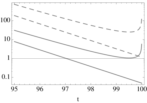
Figure 5: $M$-mode ratio $M/\mu$ (top) and Riccion mass ratio $M/\mu\sqrt{\omega}$ (bottom). Dashed lines for $M_{*}/\mu_{*}=25$ and solid lines for $M_{*}/\mu_{*}=1.05$.

We consider two scenarios one in which Riccion is realizable and other in which it is not realizable. It turns out there is bound on $M_{*}/\mu_{*}$ for each value of $t_{\rm max}$ and $N_{A}$, below which Riccion is realized in the flow, and above that bound Riccion is also outside the spectrum throughout the flow. This bound is given by,

$$\left.\frac{M_{*}}{\mu_{*}}\right|_{B}=e^{t_{\rm max}-t_{*}}\sqrt{\omega_{*}}\left(1+\frac{\omega_{1}}{\omega_{*}}\right)^{B1/2}\left(1+\frac{\omega_{2}}{\omega_{*}}\right)^{B2/2}\,.$$ (90)

This bound depends on $N_{A}$ and decreases as $N_{A}$ increases, but the dependence is very mild. For $t_{\rm max}=100$ and $N_{A}=1$, this bound is given by $M_{*}/\mu_{*}=21.51$. Thus we consider two cases: $M_{*}/\mu_{*}=1.05$ and $M_{*}/\mu_{*}=25$. In former Riccion is realized while in later Riccion is not realized throughout the whole RG trajectory for a given $N_{A}$.

For the above values of $M_{*}/\mu_{*}$, the flow of the $M^{2}/\mu^{2}$ and $M^{2}/(\omega\mu^{2})$ has been plotted in Fig. 5. For each case we note that $M$-mode is never realized throughout the flow, while Riccion is realized in one case and not in other. For $t_{\rm max}=100$, choosing $M_{*}/\mu_{*}<21.51$, we have Riccion getting realized. In the Fig. 5 we have considered the case when $M_{*}/\mu_{*}=1.05$ (solid lines), where we clearly see that Riccion is getting realized. For $M_{*}/\mu_{*}>21.51$, both $M$-mode and Riccion is out of physical spectrum throughout the whole flow. In Fig. 5 we considered the case when $M_{*}/\mu_{*}=25$ (dashed lines), where both $M$-mode and Riccion is out of physical spectrum. From Fig. 5 we notice that Riccion is physically realizable in high energy scattering processes at most for about four e-folds before $t_{max}=100$.

Throughout the whole flow within the physically allowed region (between $t_{\rm min}$ and $t_{\rm max}$), $M^{2}G$ remains small and in perturbative regime. However the beta function $M^{2}G$ is such that ultimately its flow hits a Landau singularity. Though this occurs way beyond $t_{\rm max}$. The existence of Landau singularity could be an artifact of one-loop, and might perhaps go away when higher loop corrections are incorporated. This is so because at higher loops the beta function of the coupling $1/M^{2}G$ gets a correction which is proportional to couplings instead of a constant, thereby raising the speculation that there might be a fixed point for $M^{2}G$.

The flow of $M^{2}$ and $M^{2}/\omega$ (the relative coefficients of higher-derivative terms with respect to Einstein-Hilbert term) is such that in infrared regime both $M^{2}$ and $M^{2}/\omega$ goes to infinity, thereby suppressing any higher-derivative terms, giving the Einstein-Hilbert action in the low energy regime. This can be seen more clearly from Fig. 6, where the flows of $M^{2}$ and $M^{2}/\omega$ has been depicted. This is important and crucial as then all the known low energy physics is reproduced. In the UV, $M^{2}$ goes to infinity when $t\to t_{\rm max}$, signaling that the $M$-mode goes out of physical spectrum. However the Riccion mass $M^{2}/\omega$ goes to zero, implying that the contributions from the $R^{2}$ term in the effective action becomes more prominent in the UV.

         

Figure 6: Flow of $M^{2}$ and $M^{2}/\omega$ with respect to $t$, appropriately normalized with respect to the value of $M^{2}$ and $M^{2}/\omega$ at reference point $\omega_{0}$.

Having studied the flow of the gravitational parameters in the coupled system of gauge field with higher-derivative gravity, we set back to analyze the quantum gravity correction to the gauge beta function in more detail. In general in a coupled system of gravity with gauge fields, the gauge beta function necessarily has the structure written in eq. (3), which automatically arises in perturbative study of Feynman path-integral of the coupled system. It is found that to one-loop $a=0$ in higher-derivative gravity and is independent of the gauge group. This observation has also been made in a similar one-loop computation in the context of Einstein-Hilbert gravity. It is indeed compelling to ask whether there is some deeper symmetry principle at work, responsible for vanishing of ‘$a$’-term? As this term is universal to all gauge theories (meaning independent of the gauge coupling), and is the most dominant term for small coupling, thus it is important to understand the nature of this term in more detail by isolating it in the context of abelian gauge theories without matter, where ‘$b$’ term of the beta function is absent to all loops. Simplicity of this coupled system will allow us to gain more insight in to the cause of the cancellation of divergences, leading to the vanishing of ‘$a$’-term in the gauge beta function. Therefore in the next section we will study the ‘$a$’ term in abelian gauge theory to all loops.

V Duality transformation

In this section we study abelian gauge theory coupled with gravity in order to probe into the cause of vanishing of ‘$a$’ term in the gauge beta function. Here we give a formal argument to show that $a=0$ due to the self-duality property of the abelian gauge theories in four dimensions Savit ; Peskin ; NAgauge . In this proof gravity action plays no significant role, so here we don’t explicitly specify the gravitational action. However it is important to mention that the path-integral considered should be renormalizable. We start by considering the path-integral of gauge fields coupled with gravity,

$$Z=\int{\cal D}g_{\mu\nu}\,{\cal D}A_{\rho}e^{iS_{\rm GR}}\,e^{iS_{\rm EM}}\,,$$ (91)

where $S_{\rm EM}=\left(-1/4e^{2}\right)\int{\rm d}^{4}x\,\sqrt{-g}\,g^{\mu\alpha}g^{\nu\beta}F_{\mu\nu}F_{\alpha\beta}$, and $F_{\mu\nu}=\partial_{\mu}A_{\nu}-\partial_{\nu}A_{\mu}$ and $S_{\rm GR}$ is some arbitrary renormalizable and unitary gravity action. This is important as otherwise the path-integral will not be well-defined perturbatively. For this theory the running of the gauge coupling $e^{2}$ is given by the following beta function,

$$\frac{{\rm d}}{{\rm d}t}\left(\frac{1}{e^{2}}\right)=\frac{a(\cdots)}{e^{2}}\,,$$ (92)

where the dots indicate that the function ‘$a$’ can depend upon parameters of $S_{\rm GR}$. The path-integral in eq. (91) can be re-written by making use of an auxiliary tensor field $B_{\mu\nu}$. This is done by introducing a measure for the auxiliary field in the path-integral, a determinant factor constructed exclusively from metric and modifying the original action by writing it in the first order form by making use of auxiliary field. Integrating over this auxiliary field, gives back the original path-integral. Under this transformation the path-integral becomes,

$$\int{\cal D}A_{\mu}e^{iS_{\rm EM}}=\int{\cal D}B_{\mu\nu}\,{\cal D}A_{\mu}e^{iS_{B}}\,\left[\det e^{2}G^{{\mu\nu}\alpha\beta}\right]^{1/2}\,,$$ (93)

where

$$S_{B}=e^{2}\int{\rm d}^{4}x\sqrt{-g}g^{\mu\alpha}g^{\nu\beta}B_{\mu\nu}B_{\alpha\beta}+\int{\rm d}^{4}x\,\epsilon^{{\mu\nu}\alpha\beta}B_{\mu\nu}\partial_{\alpha}A_{\beta}\,,$$ (94)

$$G^{{\mu\nu},\alpha\beta}=\sqrt{-g}(g^{\mu\alpha}g^{\nu\beta}-g^{\mu\beta}g^{\nu\alpha})\,.$$ (95)

$G^{{\mu\nu},\alpha\beta}$ is anti-symmetric in $({\mu\nu})$ and $(\alpha\beta)$ and its determinant arises after doing integration over the auxiliary field $B_{\mu\nu}$ and $\bar{\epsilon}^{{\mu\nu}\alpha\beta}$ is a four dimensional tensor density of weight $-1$. It should be noted that it is flat spacetime partial derivative that enters the second integrand of the eq. (94) (when there is covariant derivative, the connection term in the covariant derivative cancels due to the presence of $\bar{\epsilon}^{{\mu\nu}\alpha\beta}$, this happens as connection is taken to be torsionless, situation is different in presence of torsion).

On integrating the $A$ field on the rhs of eq. (93) we gets a constraint on the $B_{\mu\nu}$ field $\delta\left(\bar{\epsilon}^{{\mu\nu}\alpha\beta}\partial_{\alpha}B_{\mu\nu}\right)$. This constraint appears under the path-integration of the field $B_{\mu\nu}$. Being a $\delta$-function, this constraints the $B_{\mu\nu}$ field to pick up those configurations which satisfies $\bar{\epsilon}^{{\mu\nu}\alpha\beta}\partial_{\alpha}B_{\mu\nu}=0$. This is satisfied by solution $B_{\mu\nu}=\partial_{\mu}b_{\nu}-\partial_{\nu}b_{\mu}$. The field transformation from $B_{\mu\nu}$ to $b_{\rho}$ however introduces a jacobian constructed purely from partial derivative and Levi-civita tensor. This is a trivial normalization constant and wouldn’t affect the renormalization group study of the couplings. The path-integral for the dual-field is given by,

$$Z=C\int{\cal D}g_{\mu\nu}\,{\cal D}b_{\mu}e^{i(S_{\rm GR}+\bar{S}_{\rm EM})}\left[\det(e^{2}G^{{\mu\nu},\alpha\beta})\right]^{\frac{1}{2}}\,,$$ (96)

where $C$ is a constant and $b_{\mu}$ is the dual of $A_{\mu}$ whose action is given by,

$$\bar{S}_{\rm EM}=e^{2}\int{\rm d}^{4}x\,\sqrt{-g}g^{\mu\alpha}g^{\nu\beta}(\partial_{\mu}b_{\nu}-\partial_{\nu}b_{\mu})(\partial_{\alpha}b_{\beta}-\partial_{\beta}b_{\alpha})\,.$$ (97)

It should be noted that here we have implemented the duality transformation in the presence of metric. This dual action has also $U(1)$ gauge invariance. Next we note that the determinant of $e^{2}G^{{\mu\nu}\alpha\beta}$ which is anti-symmetric in $({\mu\nu})$ and $(\alpha\beta)$, is a general coordinate invariant ultra-local $d(d-1)/2\times d(d-1)/2$ matrix. Hence the determinant can only be proportional to some power of $\sqrt{-g}$. It is found that

$$\left(\det\left[e^{2}\sqrt{-g}(g^{\mu\alpha}g^{\nu\beta}-g^{\mu\beta}g^{\nu\alpha})\right]\right)^{1/2}=e^{d(d-1)/2}\left(\sqrt{-g}\right)^{(d-1)(d-4)/4}\,.$$ (98)

In four dimensions this is a pure number and is equal to $\left(e^{2}\right)^{3}$. Hence the dual theory path-integral looks exactly the same as the original path-integral apart from the overall constant. Perturbative renormalization group study of the dual action gives the flow of the coupling present in the dual field theory. This is given by,

$$\frac{{\rm d}}{{\rm d}t}e^{2}=a(\cdots)\,e^{2}\,,$$ (99)

where $a$ has exactly the same parameter dependence as in Eq. (92).

Compatibility of the two eqs. (92 and 99) implies that $a=0$ NAgauge . This of course comes out at one-loop level explicitly. Here we have not introduced any gauge-fixing and corresponding ghost action for the analysis. If one uses similar kind of gauge fixing conditions in the original and in the dual theory, then it is easy to show that the above proof goes through without any modification. It should be noted that this argument doesn’t depend on the gravity action or the regularization scheme, implying that in both the $U(1)$ and its dual theory, eq. (92 and 99) are inferred in any regularization scheme.

In the next section we explicitly show that at one-loop $a=0$ independent of any regularization scheme, gravity action and gauge fixing thereof.

VI Arbitrary Gravity Action

Having realized in the previous section that gravitational action play no significant role at all in the argument to show $a=0$ to all loops, it becomes all the more compulsive to see by checking whether it is indeed true in an explicit one-loop computation of the gauge beta function for arbitrary gravity action. Here in this section we do the same.

This generalization can be achieved in metric theories of gravity by considering a general action that can be constructed with metric and its derivatives. In such general theories of gravity, one can still write the form of the propagator of the metric fluctuation $h_{\mu\nu}$ around a flat background. This can be done by making use of complete set of spin projectors for rank-2 tensor field. At this step one can ask what generality in the gravitational action actually transmits to the metric fluctuation propagator around the flat background? It is noticed that higher-derivative terms of sixth order like $R^{3}$ and $R_{\mu\nu}{}^{\rho\sigma}R_{\rho\sigma}{}^{\alpha\beta}R_{\alpha\beta}{}^{\mu\nu}$ don’t contribute to the propagator but terms like $R\Box R$ (which has same order of derivatives) contribute. This observation brings to realization that terms of action which are at most quadratic in curvature, contributes to the propagator of the $h_{\mu\nu}$ field. Denoting the inverse propagator of the $h_{\mu\nu}$ field by $\Delta_{G}^{{\mu\nu}\alpha\beta}$ as in eq. (32), the most general form of it in momentum space can be written as,

$$\Delta_{G}^{{\mu\nu}\alpha\beta}(p)=\sum_{i}\,\tilde{Y}_{i}(p^{2})P_{i}^{{\mu\nu}\alpha\beta}\,,$$ (100)

where $i=\{2,1,s,w,sw,ws\}$, $P_{i}$’s are all the projectors as given in appendix A. By making use of the properties of these projectors, this can be inverted to obtain the expression for the most general propagator around the flat background of the $h_{\mu\nu}$ field. This can be written as,

$$D^{{\mu\nu}\rho\sigma}=\sum_{i}\,Y_{i}(p^{2})P_{i}^{{\mu\nu}\alpha\beta}\,,$$ (101)

where $Y_{i}$ are propagators for various spin components and are related to to $\tilde{Y}_{i}$’s in the following way,

$$Y_{2}=\frac{1}{\tilde{Y}_{2}}\,,\hskip 14.22636ptY_{1}=\frac{1}{\tilde{Y}_{1}}\,,\hskip 14.22636ptY_{s}=\frac{\tilde{Y}_{w}}{\tilde{Y}_{s}\tilde{Y}_{w}-\tilde{Y}_{sw}\tilde{Y}_{ws}}\,,$$

$$Y_{w}=\frac{\tilde{Y}_{s}}{\tilde{Y}_{s}\tilde{Y}_{w}-\tilde{Y}_{sw}\tilde{Y}_{ws}}\,,\hskip 14.22636ptY_{sw}=-\frac{\tilde{Y}_{sw}}{\tilde{Y}_{s}\tilde{Y}_{w}-\tilde{Y}_{sw}\tilde{Y}_{ws}}\,,\hskip 14.22636ptY_{ws}=-\frac{\tilde{Y}_{ws}}{\tilde{Y}_{s}\tilde{Y}_{w}-\tilde{Y}_{sw}\tilde{Y}_{ws}}\,.$$ (102)

In the case of higher-derivative gravity in Landau gauge we have only $Y_{2}$ and $Y_{s}$. However in a general gauge fixing and for an arbitrary gravity action all the $Y_{i}$’s will be present.

Using this as the propagator for the fluctuation field $h_{\mu\nu}$, one can repeat the computation of the charge renormalization at one-loop for arbitrary gravity action. This can be done along the same lines as in section. III. Again we will have two diagrams giving quantum gravity contribution to the gauge coupling: tadpole and bubble, except now we have a general propagator for the $h_{\mu\nu}$ field. This generality also encapsulates within itself the arbitrariness in the choice of gauge fixing parameters for the gravity side.

Following the steps as in subsection. III.4.1 and III.4.2, we compute the contributions of the tadpole and bubble diagram respectively. Reaching the stage when momentum integration needs to be performed (as in eqs. (57 and 69)), we argue that as the measure and the integrand is a Lorentz covariant quantity, therefore under the momentum integral the tensorial part of integrand consisting of various combinations of four momenta $p_{\mu}$ (which is the momentum variable), can be replaced by a combination of flat background metric $\eta_{\mu\nu}$, with various coefficients, obeying the symmetries of the integrand. This is then contracted with the vertices to obtain the equations similar to eqs. (58 and 70).

In the case of tadpole the vertex $V^{\rho\sigma{\mu\nu}}_{\theta\tau\alpha\beta}$ (given in the appendix B) is used to contract with different combination of $\eta_{\mu\nu}$ for various spin-projectors to yield,

$$\Gamma_{{\rm Tad}}=-\frac{i}{8e^{2}}\int\,{\rm d}^{d}x\bar{F}^{a}_{{\mu\nu}}\bar{F}^{a{\mu\nu}}\,\int\,\frac{{\rm d}^{d}p}{(2\pi)^{d}}\sum_{i}Y_{i}(p^{2})\biggl{[}\frac{(d-4)(d-6)}{4}H_{i}-\frac{d^{2}-8d+4}{2}G_{i}\biggr{]}\,,$$ (103)

where the coefficients $H_{i}$ and $G_{i}$ corresponding to various spin-projectors are given in appendix C. For bubble diagram we use the properties of the vertex $V^{a{\mu\nu}\alpha\beta}$ which is symmetric is first two greek index and anti-symmetric in last two greek index, to obtain the result. These properties are discussed in appendix B. The contribution of the bubble diagram is given by,

$$\Gamma_{{\rm Bub}}=\frac{i}{8e^{2}}\int{\rm d}^{d}x\bar{F}^{a{\mu\nu}}\bar{F}^{a}_{{\mu\nu}}\int\frac{{\rm d}^{d}p}{(2\pi)^{d}}\sum_{i}Y_{i}(p^{2})$$

$$\times\biggl{[}(d-4)^{2}A_{i}+2(5d-8)B_{i}-2(d-4)(d-1)\left(C_{i}+D_{i}\right)+4(d^{2}-4d+6)E_{i}\,,\biggr{]}$$ (104)

where the coefficients $A_{i}$’s, $B_{i}$’s, $C_{i}$’s, $D_{i}$’s and $E_{i}$’s for various spin projectors are obtained in appendix C. Adding the tadpole and bubble contribution after plugging the various coefficients ($A$, $B$, $C$, $D$, $E$, $G$ and $H$) we find,

$$\Gamma_{{\rm Grav}}=-\frac{i(d-4)\Omega(d)}{8e^{2}}\int{\rm d}^{d}x\,{\rm tr}F^{2}\,,\hskip 14.22636pt{\rm where\,\,\,}\Omega(d)=\sum_{i}\Omega_{i}\int\frac{{\rm d}^{d}p}{(2\pi)^{d}}Y_{i}(p^{2})\,,$$ (105)

and various coefficients $\Omega_{i}$’s are just functions of space-time dimension $d$ and are given by,

$$\Omega_{2}=-\frac{(d-5)(d-2)(d+1)}{4d(d-1)}\,,\hskip 14.22636pt\Omega_{1}=-\frac{d-1}{8d}\,,$$

$$\Omega_{s}=\frac{d^{2}-12d+19}{4d(d-1)}\,,\hskip 14.22636pt\Omega_{sw}=\Omega_{ws}=\frac{\sqrt{d-1}}{4d}\,.$$ (106)

From the total contribution of the two diagrams obtained in eq. (105) we note that irrespective of the propagator of the $h_{\mu\nu}$ field, this full quantum gravity contribution to gauge field action is always proportional to $(d-4)$. This is independent of the gravity action and the gauge fixing. This arbitrariness is present in the various $Y_{i}$’s and doesn’t affect the overall factor of $(d-4)$. It is independent of the regularization scheme as we have not performed the momentum integration. In deriving this result we only used the Lorentz covariance of the integrand present in the loop integral. It should also be noted that this one-loop contribution is also independent of the symmetry group of the gauge field. Therefore to one-loop we find that $a=0$ for arbitrary gravity action and gauge fixing. It is also independent of regularization scheme and the symmetry group of the gauge field. This further justifies the observation made in sec. V where it was found that $a=0$ to all loops. Moreover, as the graviton propagator is kept arbitrary here, therefore it also implies that subclass of higher-loop diagrams, which involves graviton self energy corrections as sub-graphs (corrections to graviton propagator in diagrams (c) and (d) of Fig. 2), will also cancel each other in four spacetime dimensions. Some of such diagrams at two loops are presented in Fig. 3, where the graviton propagator has undergone self energy correction.

VII Discussion and Conclusion

In this paper we study gauge fields coupled with higher-derivative gravity, which has been shown to be perturbatively renormalizable in four dimensions Stelle ; Fradkin ; Moriya . However higher-derivative gravity is plagued with the problem of unitarity. This problem is manifestly apparent when the propagator of the metric fluctuation field $h_{\mu\nu}$ is written around a flat background. There it is clearly noticed, the presence of negative norm states, namely the propagator of the spin-2 massive mode appears with the wrong sign, and thus violates unitarity at tree level. This problem of unitarity has recently been studied again in the light of quantum corrections NarainA1 ; NarainA2 , where it was found that in a certain domain of coupling parameter space (which is large enough to incorporate the known physics), the one-loop running of gravitational parameters makes the mass of spin-2 massive mode run in such a way so that it is always above the energy scale being probed. In other words under quantum corrections the pole in the propagator of the $M$-mode disappears. This one-loop result was a major boost for further study and led to us investigating the coupling of higher-derivative gravity with gauge fields in NAgauge . In NAgauge quantum gravity correction to charge renormalization was studied, and major results were presented. Here we present the details of the computation and discuss the unitarity in the coupled system.

The path-integral of the coupled system of gauge field with higher-derivative gravity is completely well defined in $4-\epsilon$ dimensions, where it is perturbatively studied in the dimensional regularization scheme. One-loop computation of the charge renormalization shows that there is no quantum gravity correction to the gauge coupling beta function. This coupled system being renormalizable and free from quadratic divergences evades the criticism raised in Donoghue1 .

Generically, in perturbation theory, the coupled gauge-gravity system will lead to the gauge coupling beta function consisting of two kinds of terms: ‘$a$’ and ‘$b$’ as shown in eq. (3). It is argued in the paper that the ‘$a$’ term is universal to all gauge theories in the sense that it is independent of the gauge coupling $e^{2}$, but depends on the gravitational parameters and the information content of the matter sector. On the other hand the ‘$b$’ term is not universal. In this paper our intentions were to study the nature of this ‘$a$’ term to all loops in four dimensions.

One-loop computation showed no quantum gravity contribution to the gauge coupling beta function thereby implying vanishing of ‘$a$’ term in four dimensions. Moreover it was found to be zero for all metric theories of gravity and furthermore is independent of gauge group, regularization scheme and gauge fixing condition. Universality of this ‘$a$’ term allowed us to isolate it by studying it in the context of simple abelian gauge theories without matter in four dimensions. However self-duality of abelian gauge theories in four dimensions opened another window, which allowed us to look at the same problem from a different angle. Motivated by this realization, we performed duality transformation by making use of an auxiliary field to study the flow of the coupling in the dual theory. In the case of abelian gauge theories, the dual theory is also abelian (self-duality), except that the coupling in front of gauge field action changes from $1/e^{2}$ to $e^{2}$ respectively. The beta function of the gauge coupling in the dual theory has the same structure as in the case of original theory with the same ‘$a$’-term, as the gravity action is same. The only way two equations for running of $e^{2}$ can be satisfied is when ‘$a$’-term vanishes. This is an all-loop argument and is independent of the gravity action. However it is only for higher-derivative gravity that the path-integral of the coupled system is renormalizable and well defined.

We also studied the unitarity of the coupled system of gauge fields with higher-derivative gravity at one-loop. The beta functions of the of the gravitational couplings gets corrected due to the presence of gauge fields. It is realized that only positive $\omega$ is allowed and describes the physical domain. This requirement puts a upper and lower bound on the renormalization group time $t$ that is allowed by physical domain of $\omega$. Thus the parameters only flow between $t_{\rm min}$ and $t_{\rm max}$. For $t<t_{\rm min}$, $\omega$ becomes negative, signaling the instability of the vacuum, meaning that one enters a regime where effects of cosmological constant should be taken into account. For $t>t_{\rm max}$ one-loop equation for $\omega$ doesn’t have a solution. This could be an artifact of the one-loop results and might perhaps go away when higher loop corrections are incorporated.

The flow of $G$ is such that it goes to zero in both extremes of RG time $t$. In $\omega$-space, $G\sim 1/\omega$ in the UV, which is a gauge parameter invariant result and is also independent of whether gauge fields are present or not. In the IR however, $G\sim\omega^{7/20}$ and this is gauge parameter dependent, in the sense that the power with which it goes to zero depends on gauge condition. The one-loop beta functions of gravitational parameters allow us to compute the running of $M^{2}/\mu^{2}$, flow of which has a minima at the point $\omega_{*}$. Demanding that the value of $M^{2}/\mu^{2}$ at minima is greater than one, assures that throughout the RG evolution it will remain greater than one. This can be arranged easily by choosing the initial parameters appropriately. Once this condition is satisfied, it guarantees that the RG trajectory will be unitary as in NarainA1 ; NarainA2 . Thus the coupled system of gauge field with higher-derivative gravity can be made unitary in this domain of coupling parameter space. Similarly working out the flow of $M^{2}/\omega\mu^{2}$ using the one-loop beta functions of the gravitational parameters, it is found that it is a monotonically decreasing function of RG time $t$. Choice of initial parameters further decides whether Riccion will be physically realizable or not. Thus the physical theory will consist of gravitons and gauge bosons either with Riccions or without them. The flow of $M^{2}$ and $M^{2}/\omega$ is such that in low energy the higher-derivative terms are naturally suppressed favoring the Einstein-Hilbert and cosmological constant term.

Having realized that the coupled system being renormalizable and unitary, it becomes all the more important to study charge renormalization in this system. Finding that $a=0$ to all loops, results in dramatic consequences, meaning that photons interacting only with metric fluctuations will propagate essentially as free particle at short distances. This is a consequence of self-duality property of abelian gauge field action. However it should be mentioned that there is indeed finite charge renormalization, which decreases the coupling, but this is of no significance when matter fields are present. In case of non-abelian gauge fields, the same phenomenon manifests as there will not be any ‘$a$’ term, but the running is controlled by the ‘$b$’-term.

In the absence of ‘$a$’-term, the leading contribution to the running of gauge coupling comes from the ‘$b$’-term of the beta function. At one-loop the ‘$b$’-term is completely independent of the gravitational parameters i.e. it is solely a consequence of charge interactions alone. However at two-loops things change. In the gauge coupling beta function there is not only matter contributions (which do not change the behavior of running gauge coupling compared to one-loop result), but also contributions which have both gauge and gravity couplings. These can influence the behavior of the running gauge coupling by giving rise to new fixed points etc. This can open new avenues to our understanding of gravity and gauge field theories. Further higher-loop corrections from gauge fields will also influence the gravitational sector. It will interesting to know how the Landau singularity both in the $U(1)$ gauge theory and higher-derivative gravity sector (weyl-square coupling) gets affected under the influence of higher-loop corrections? This will be the subject of future work.

Acknowledgements

GN would like to thank Romesh Kaul for useful discussions.

Appendix A Projectors

The metric fluctuation field $h_{\mu\nu}$ around a general background can be decomposed into various components by doing a transverse-traceless decomposition. This is equivalent to doing decomposition of a vector into transverse and longitudinal components. For the metric fluctuation field $h_{\mu\nu}$ around a flat background, this decomposition can be written in momentum space as,

$$h_{{\mu\nu}}=h^{T}_{{\mu\nu}}+\iota\left(q_{\mu}\xi_{\nu}+q_{\nu}\xi_{\mu}\right)+\left(\eta_{\mu\nu}-\frac{q_{\mu}q_{\nu}}{q^{2}}\right)s+\frac{q_{\mu}q_{\nu}}{q^{2}}\,w\,,$$ (107)

where the various components satisfies the following constraints,

$$h^{T}_{\mu}{}^{\mu}=0\,,\hskip 14.22636ptq^{\mu}h^{T}_{\mu\nu}=0\,,\hskip 14.22636ptq^{\mu}\xi_{\mu}=0\,.$$ (108)

Here $h^{T}_{\mu\nu}$ is a transverse-traceless symmetric tensor, $\xi_{\mu}$ is a transverse vector and $s$ and $w$ are two scalars. This decomposition can be neatly written by making use of flat spacetime projectors, which projects various components of $h_{\mu\nu}$ field into $h^{T}_{\mu\nu}$, $\xi_{\mu}$, $s$ and $w$ respectively. These projectors are written in terms of the following two projectors,

$$L_{\mu\nu}=\frac{q_{\mu}\,q_{\nu}}{q^{2}}\,\ ,\hskip 28.45274ptT_{\mu\nu}=\eta_{{\mu\nu}}-\frac{q_{\mu}\,q_{\nu}}{q^{2}}\,,$$ (109)

which are basically the projector for projecting out various components of a vector field. They satisfy $q^{\mu}T_{\mu\nu}=0$ and $q^{\mu}L_{\mu\nu}=q_{\nu}$. Using them the projectors for the rank-2 tensor field can be constructed. These are given by,

$$(P_{2})_{\mu\nu}{}^{\alpha\beta}=\frac{1}{2}\left[T_{\mu}{}^{\alpha}T_{\nu}{}^{\beta}+T_{\mu}{}^{\beta}T_{\nu}{}^{\alpha}\right]-\frac{1}{d-1}T_{\mu\nu}T^{\alpha\beta}\,,$$ (110)

$$(P_{1})_{\mu\nu}{}^{\alpha\beta}=\frac{1}{8}\left[T_{\mu}{}^{\alpha}\,L_{\nu}{}^{\beta}+T_{\mu}{}^{\beta}\,L_{\nu}{}^{\alpha}+T_{\nu}{}^{\alpha}\,L_{\mu}{}^{\beta}+T_{\nu}{}^{\beta}\,L_{\mu}{}^{\alpha}\right]\,,$$ (111)

$$(P_{s})_{\mu\nu}{}^{\alpha\beta}=\frac{1}{d-1}T_{\mu\nu}\,T^{\alpha\beta}\,,$$ (112)

$$(P_{w})_{\mu\nu}{}^{\alpha\beta}=L_{\mu\nu}\,L^{\alpha\beta}\,.$$ (113)

The projectors for spin-2, spin-1, spin-s and spin-w form an orthogonal set. In the scalar sector there are two more projectors (which are not projectors in the strict sense), which along with spin-s and spin-w projectors form a complete set. They are given by,

$$(P_{sw})_{\mu\nu}{}^{\alpha\beta}=\frac{1}{\sqrt{d-1}}T_{\mu\nu}\,L^{\alpha\beta}\,,$$ (114)

$$(P_{ws})_{\mu\nu}{}^{\alpha\beta}=\frac{1}{\sqrt{d-1}}L_{\mu\nu}\,T^{\alpha\beta}\,.$$ (115)

The projectors in eqs. (110, 111, 112 and 113) forms a complete set in the sense that their sum is unity.

$$(P_{2})_{\mu\nu}{}^{\rho\sigma}+(P_{1})_{\mu\nu}{}^{\rho\sigma}+(P_{s})_{\mu\nu}{}^{\rho\sigma}+(P_{w})_{\mu\nu}{}^{\rho\sigma}=\delta_{\mu\nu}^{\rho\sigma}\,,$$ (116)

where $\delta_{\mu\nu}^{\rho\sigma}=1/2(\delta_{\mu}^{\rho}\delta_{\nu}^{\sigma}+\delta^{\rho}_{\nu}\delta^{\sigma}_{\mu})$. Each of these projectors when act of $h_{\mu\nu}$ projects out various spin components of the tensor field.

$$(P_{2})_{{\mu\nu}}{}^{\rho\sigma}\,h_{\rho\sigma}=h_{{\mu\nu}}^{T}\,,\hskip 14.22636pt(P_{1})_{{\mu\nu}}{}^{\rho\sigma}\,h_{\rho\sigma}=\iota\left(q_{\mu}\xi_{\nu}+q_{\nu}\xi_{\mu}\right)\,,$$

$$(P_{s})_{{\mu\nu}}{}^{\rho\sigma}\,h_{\rho\sigma}=(d-1)T_{\mu\nu}s\,,\hskip 14.22636pt(P_{s})_{{\mu\nu}}{}^{\rho\sigma}\,h_{\rho\sigma}=L_{\mu\nu}w\,.$$ (117)

If the projectors $P_{2}$, $P_{1}$, $P_{s}$ and $P_{w}$ are written as $P_{22}$, $P_{11}$, $P_{ss}$ and $P_{ww}$ respectively, then all the projectors (including $P_{sw}$ and $P_{ws}$) satisfy the following algebra,

$$P_{ij}P_{mn}=\delta_{jm}P_{in}\,,$$ (118)

where $i$, $j$, $m$ and $n$= {$2$, $1$, $s$, $w$}.

Now we study the contraction of spin projectors of $h_{\mu\nu}$ with various tensors. For this we first consider the trace of projectors $T$ and $L$. This is given by,

$${\rm Tr}\,L_{\mu\nu}=1\,,\hskip 28.45274pt{\rm Tr}\,T_{\mu\nu}=d-1\,.$$ (119)

Using this and properties of the various projectors satisfying the algebra in eq. (118), we obtain the contraction of the projectors with various tensors constructed with $\eta_{\mu\nu}$ and momentum $q_{\mu}$, which are used in the one-loop computation of the paper. These tensor are given by,

$$\eta_{\mu\nu}\eta_{\rho\sigma},\hskip 14.22636pt(\eta_{\mu\rho}\eta_{\nu\sigma}+\eta_{\mu\sigma}\eta_{\nu\rho}),\hskip 14.22636pt\frac{q_{\rho}q_{\sigma}}{q^{2}}\eta_{\mu\nu},\hskip 14.22636pt\eta_{\rho\sigma}\frac{q_{\mu}q_{\nu}}{q^{2}},$$

$$U_{{\mu\nu}\rho\sigma\gamma\theta}=\left(\eta_{\rho\mu}\eta_{\nu\gamma}\eta_{\sigma\theta}+\eta_{\rho\nu}\eta_{\mu\gamma}\eta_{\sigma\theta}+\eta_{\sigma\mu}\eta_{\nu\gamma}\eta_{\rho\theta}+\eta_{\sigma\nu}\eta_{\mu\gamma}\eta_{\rho\theta}+\eta_{\rho\mu}\eta_{\nu\theta}\eta_{\sigma\gamma}+\eta_{\rho\nu}\eta_{\mu\theta}\eta_{\sigma\gamma}\right.$$

$$\left.+\eta_{\sigma\mu}\eta_{\nu\theta}\eta_{\rho\gamma}+\eta_{\sigma\nu}\eta_{\mu\theta}\eta_{\rho\gamma}\right)$$ (120)

And the contraction of these tensors with the various spin-projectors are given in Table. 1.

	$\left(P_{2}\right)_{{\mu\nu}\rho\sigma}$	$\left(P_{1}\right)_{{\mu\nu}\rho\sigma}$	$\left(P_{s}\right)_{{\mu\nu}\rho\sigma}$	$\left(P_{sw}\right)_{{\mu\nu}\rho\sigma}$	$\left(P_{ws}\right)_{{\mu\nu}\rho\sigma}$	$\left(P_{w}\right)_{{\mu\nu}\rho\sigma}$
$\eta^{{\mu\nu}}\eta^{\rho\sigma}$	0	0	d-1	$\sqrt{d-1}$	$\sqrt{d-1}$	1
$(\eta^{\mu\rho}\eta^{\nu\sigma}+\eta^{\nu\rho}\eta^{\mu\sigma})$	$(d+1)(d-2)$	$\frac{d-1}{2}$	2	0	0	2
$2(q^{\rho}q^{\sigma}/q^{2})\eta^{\mu\nu}$	0	0	0	0	$2\sqrt{d-1}$	2
$2\eta^{\rho\sigma}(q^{\mu}q^{\nu}/q^{2})$	0	0	0	$2\sqrt{d-1}$	0	2
$(q_{\gamma}q_{\theta}/q^{2})U^{{\mu\nu}\rho\sigma\gamma\theta}$	0	d-1	0	0	0	8

Table 1: Contraction of projectors with various tensors

Appendix B Gauge Vertices and propagator

The one-loop quantum gravity correction to the gauge beta function can be obtained by doing second variation of the coupled action with respect to various fields. While the gravity part of the action gives the propagator of the fluctuation field $h_{\mu\nu}$ around the flat background, the gauge field action when varied gives the gauge field propagator, and various vertices that are used in this one-loop computation. In the following we will write the various vertices arising from the gauge field action and the gauge field propagator. After obtaining these vertices we will study the contraction of these vertices with various tensor. Such contractions are ultimately used in the computation of the two diagrams that give the one-loop quantum gravity contribution to the gauge beta function.

B.1 Gauge-Gauge vertices

The second variation of the gauge field action with respect to gauge field, gives rise to gauge field propagator and gauge-gauge vertices relevant for the one-loop computation. These vertices arise only for non-abelian gauge theories and for abelian gauge theories they are absent. The presence of these vertices (which are coming due to self interaction of non-abelian gauge field) is responsible for asymptotic freedom of gauge coupling in non-gravitational scenarios. Here we write these vertices for completeness, while it will not be needed in our one-loop computation of the quantum gravity correction to gauge beta function.

Expanding the gauge field action eq. (2) up to second order in the fluctuation field ${\cal A}_{\mu}$ (where $A_{\mu}=\bar{A}_{\mu}+{\cal A}_{\mu}$), we get the expression for the gauge field propagator and gauge-gauge vertices. This is written in the last line of eq. (III.3). After some manipulations it acquires the following simplified form,

$$-\frac{1}{8e^{2}}\int{\rm d}^{d}x\biggl{[}4\mathcal{A}^{a\mu}\biggl{\{}-\eta_{\mu\nu}\delta^{ac}\Box-2f^{abc}\eta_{\mu\nu}\left(\partial_{\rho}\bar{A}^{b\rho}+\bar{A}^{b\rho}\partial_{\rho}\right)+\eta_{\mu\nu}f^{abc}f^{ecb}\bar{A}^{d}_{\rho}\bar{A}^{e\rho}\biggr{\}}\mathcal{A}^{c\nu}$$

$$+4\mathcal{A}^{a\nu}D_{\nu}D_{\mu}\mathcal{A}^{a\mu}+4f^{abc}\bar{F}^{a}_{\mu\nu}\mathcal{A}^{b\mu}\mathcal{A}^{c\nu}\biggr{]}\,.$$ (121)

To this the gauge fixing action given in eq. (11) is added. This gives the gauge field propagator and various vertices relevant for one-loop computation.

$$-\frac{1}{8e^{2}}\int{\rm d}^{d}x\mathcal{A}^{a\mu}\biggl{[}\left(\Delta_{g}\right)^{ac}_{\mu\nu}+\left(\Delta_{1}\right)^{ac}_{\mu\nu}+\left(\Delta_{2}\right)^{ac}_{\mu\nu}+\left(\Delta_{3}\right)^{ac}_{\mu\nu}\biggr{]}\mathcal{A}^{c\nu}$$ (122)

where,

$$\left(\Delta_{g}\right)^{ac}_{\mu\nu}=4\delta^{ac}\left[-\eta_{\mu\nu}\Box+\left(1-\frac{1}{\xi}\right)\partial_{\mu}\partial_{\nu}\right]\,,$$

$$\left(\Delta_{1}\right)^{ac}_{\mu\nu}=-8f^{abc}\left\{\eta_{\mu\nu}\left(\partial_{\rho}\bar{A}^{b\rho}+\bar{A}^{b\rho}\partial_{\rho}\right)+\left(1-\frac{1}{\xi}\right)\left(\partial_{\mu}\bar{A}^{b}_{\nu}+\bar{A}^{b}_{\nu}\partial_{\mu}\right)\right\}$$

$$\left(\Delta_{2}\right)^{ac}_{\mu\nu}=4f^{abc}f^{ecb}\left\{\eta_{\mu\nu}\bar{A}^{d}_{\rho}\bar{A}^{e\rho}-\left(1-\frac{1}{\xi}\right)\bar{A}^{d}_{\mu}\bar{A}^{e}_{\nu}\right\}\,,$$

$$\left(\Delta_{3}\right)^{ac}_{\mu\nu}=-8f^{abc}F^{b}_{\mu\nu}\,.$$ (123)

From the above we note that $(\Delta_{g})^{ac}_{\mu\nu}$ is the inverse gauge propagator while $\Delta_{1}$, $\Delta_{2}$ and $\Delta_{3}$ are the gauge-gauge vertices.

B.2 Gauge-Gravity vertices

At the one-loop level the gauge-gravity vertices arise from the following term of the second variation of the gauge field action given in eq. (III.3). This arises from the variation of gauge field action in eq. (2) once with respect to $h_{\mu\nu}$ and once with respect to ${\cal A}_{\rho}^{a}$. This is given by,

$$-\frac{1}{8e^{2}}\int{\rm d}^{d}x\left(2h\eta^{\mu\alpha}\eta^{\nu\beta}-8h^{\mu\alpha}\eta^{\nu\beta}\right)\left(D_{\mu}\mathcal{A}^{a}_{\nu}-D_{\nu}\mathcal{A}^{a}_{\mu}\right)\bar{F}^{a}_{\alpha\beta}$$ (124)

This can be simplified and re-written in the following form after doing integration by parts in some terms. This vertex in then given by,

$$=-\frac{1}{8e^{2}}\int{\rm d}^{d}x\,\biggl{[}2h_{\mu\nu}V^{a\mu\nu\gamma^{\prime}\gamma}D_{\gamma^{\prime}}\mathcal{A}^{a}_{\gamma}-2\mathcal{A}^{a}_{\gamma}V^{a\mu\nu\gamma^{\prime}\gamma}D_{\gamma^{\prime}}h_{\mu\nu}-2A^{a}_{\gamma}D_{\gamma^{\prime}}V^{a\mu\nu\gamma^{\prime}\gamma}h_{\mu\nu}\biggr{]}$$ (125)

where,

$$V^{a\mu\nu\gamma^{\prime}\gamma}=\biggl{[}\eta^{\mu\nu}F^{\gamma^{\prime}\gamma}-\left(\eta^{\mu\gamma^{\prime}}\bar{F}^{a\nu\gamma}+\eta^{\nu\gamma^{\prime}}\bar{F}^{a\mu\gamma}-\eta^{\mu\gamma}\bar{F}^{a\nu\gamma^{\prime}}-\eta^{\nu\gamma}\bar{F}^{a\mu\gamma^{\prime}}\right)\biggr{]}$$ (126)

From this we note that $V^{a{\mu\nu}\gamma,\gamma}$ is symmetric is ${\mu\nu}$ and anti-symmetric in $\gamma^{\prime}\gamma$. In these kind of vertices there is one internal gluon line ${\cal A}_{\gamma}^{a}$, one internal metric fluctuation $h_{\mu\nu}$ line and one external gluon line, here given by $\bar{F}_{\mu\nu}$.

B.3 Gravity-Gravity vertices from gauge action

From the second variation of the gauge field action given in eq. (III.3) we obtain the interaction vertex with two internal metric fluctuation $h_{\mu\nu}$ line and two external $\bar{F}$ lines. This is obtained by varying the gauge field action given in eq. (2) twice with respect to $h_{\mu\nu}$ field. This is given by,

$$-\frac{1}{8e^{2}}\int{\rm d}^{d}x\biggl{\{}\left(\frac{1}{4}h^{2}-\frac{1}{2}h_{\mu\nu}h^{\mu\nu}\right)g^{\mu\alpha}g^{\nu\beta}-2hh^{\mu\alpha}g^{\nu\beta}+4h^{\mu\rho}h_{\rho}{}^{\alpha}g^{\nu\beta}+2h^{\mu\alpha}h^{\nu\beta}\biggr{\}}F_{\mu\nu}^{a}F_{\alpha\beta}^{a}$$ (127)

$$=-\frac{1}{8e^{2}}\int{\rm d}^{d}x\biggl{[}h_{\mu\nu}\biggl{\{}\frac{1}{4}\left(\eta^{\mu\nu}\eta^{\rho\sigma}-\eta^{\mu\rho}\eta^{\nu\sigma}-\eta^{\mu\sigma}\eta^{\nu\rho}\right)\eta_{\theta\alpha}\eta_{\tau\beta}-\eta^{\rho\sigma}\eta_{\tau\beta}\left(\delta^{\mu}_{\theta}\delta^{\nu}_{\alpha}+\delta^{\nu}_{\theta}\delta^{\mu}_{\alpha}\right)$$

$$+2\delta^{\sigma}_{\alpha}\eta_{\tau\beta}\left(\delta^{\mu}_{\theta}\eta^{\rho\nu}+\delta^{\nu}_{\theta}\eta^{\mu\rho}\right)+\frac{1}{2}\left(\delta^{\mu}_{\theta}\delta^{\nu}_{\alpha}+\delta^{\nu}_{\theta}\delta^{\mu}_{\alpha}\right)\left(\delta^{\rho}_{\tau}\delta^{\sigma}_{\beta}+\delta^{\rho}_{\beta}\delta^{\sigma}_{\tau}\right)\biggr{\}}h_{\rho\sigma}\biggr{]}F_{\theta\tau}^{a}F_{\alpha\beta}^{a}$$

$$=-\frac{1}{8e^{2}}\int{\rm d}^{d}x\,\,h_{\mu\nu}V^{\mu\nu\rho\sigma}_{\theta\tau\alpha\beta}\bar{F}^{a\theta\tau}\bar{F}^{a\alpha\beta}h_{\rho\sigma}\,,$$

where,

$$V^{\mu\nu\rho\sigma}_{\theta\tau\alpha\beta}=\biggl{\{}\frac{1}{4}\left(\eta^{\mu\nu}\eta^{\rho\sigma}-\eta^{\mu\rho}\eta^{\nu\sigma}-\eta^{\mu\sigma}\eta^{\nu\rho}\right)\eta_{\theta\alpha}\eta_{\tau\beta}-\eta^{\rho\sigma}\eta_{\tau\beta}\left(\delta^{\mu}_{\theta}\delta^{\nu}_{\alpha}+\delta^{\nu}_{\theta}\delta^{\mu}_{\alpha}\right)$$

$$+2\delta^{\sigma}_{\alpha}\eta_{\tau\beta}\left(\delta^{\mu}_{\theta}\eta^{\rho\nu}+\delta^{\nu}_{\theta}\eta^{\mu\rho}\right)+\frac{1}{2}\left(\delta^{\mu}_{\theta}\delta^{\nu}_{\alpha}+\delta^{\nu}_{\theta}\delta^{\mu}_{\alpha}\right)\left(\delta^{\rho}_{\tau}\delta^{\sigma}_{\beta}+\delta^{\rho}_{\beta}\delta^{\sigma}_{\tau}\right)\biggr{\}}$$ (128)

B.4 Properties of Gauge-gravity vertex

Having obtained the various vertices that will be needed for the one-loop computation of the quantum gravity contribution to the gauge beta function, we set to study their properties by contracting them with various tensors. These will be very useful in doing the computation of the tadpole and bubble diagrams in sections. III.4.1 and III.4.2 respectively. These properties are given as follows,

$$\eta_{\alpha\beta}V^{c\alpha\beta\gamma^{\prime}\gamma}=(d-4)\bar{F}^{c\gamma^{\prime}\gamma}\,,$$ (131)

$$\eta_{\beta\gamma^{\prime}}V^{c\alpha\beta\gamma^{\prime}\gamma}=-(d-1)\bar{F}^{c\alpha\gamma}\,,$$

$$(\eta_{\rho\alpha}\eta_{\sigma\beta}+\eta_{\rho\beta}\eta_{\sigma\alpha})\eta_{\gamma^{\prime}\theta}\eta_{\tau\gamma}V^{c\alpha\beta\gamma^{\prime}\gamma}V^{c\rho\sigma\theta\tau}=2V^{c\alpha\beta\gamma^{\prime}\gamma}V^{c}{}_{\alpha\beta\gamma^{\prime}\gamma}=2(5d-8)\bar{F}^{a{\mu\nu}}\bar{F}^{a}_{{\mu\nu}}\,,$$

$$(\eta_{\rho\gamma^{\prime}}\eta_{\sigma\theta}+\eta_{\rho\theta}\eta_{\sigma\gamma^{\prime}})\eta_{\alpha\beta}\eta_{\tau\gamma}V^{c\alpha\beta\gamma^{\prime}\gamma}V^{c\rho\sigma\theta\tau}=-2(d-4)(d-1)\bar{F}^{a{\mu\nu}}\bar{F}^{a}_{{\mu\nu}}\,,$$ (134)

$$(\eta_{\alpha\gamma^{\prime}}\eta_{\beta\theta}+\eta_{\beta\gamma^{\prime}}\eta_{\alpha\theta})\eta_{\rho\sigma}\eta_{\tau\gamma}V^{c\alpha\beta\gamma^{\prime}\gamma}V^{c\rho\sigma\theta\tau}=-2(d-4)(d-1)\bar{F}^{a{\mu\nu}}\bar{F}^{a}_{{\mu\nu}}\,,$$

$$U_{\rho\sigma\alpha\beta\gamma^{\prime}\theta}\eta_{\tau\gamma}V^{c\alpha\beta\gamma^{\prime}\gamma}V^{c\rho\sigma\theta\tau}=4(d^{2}-4d+6)\bar{F}^{a{\mu\nu}}\bar{F}^{a}_{{\mu\nu}}\,.$$

where $U_{\rho\sigma\alpha\beta\gamma\theta}$ is defined in eq. (A).

Appendix C Momentum Integrals

Here we will do the computation of the momentum integrals that are witnessed during the process of evaluating the tadpole and bubble graph in section. III.4.1 and III.4.2 respectively. The important thing to realize in the evaluation of these integration is that the actual momentum integrals are Lorentz covariant quantities. Therefore any tensor structure appearing in the integrands (made of momentum integration variable), after the integration, will result in Lorentz covariant quantity constructed using background flat spacetime metric $\eta_{\mu\nu}$. This is equivalent to replacing the integrand with the same tensor structure constructed with flat metric $\eta_{\mu\nu}$. This simplifies the integration process very much and in the end leads to evaluation of scalar integrals multiplied by various combination of flat metric $\eta_{\mu\nu}$.

In the case of tadpole graph, the following momentum integral is witnessed,

$$\int\,\frac{{\rm d}^{d}p}{(2\pi)^{d}}\,\sum_{i}\,Y_{i}(p^{2})\left(P_{i}\right)_{{\mu\nu}\rho\sigma}(p)\,,$$ (135)

where $i={2,1,s,w,sw,ws}$. Under the $p$-integration we replace $P_{i}$’s as

$$\left(P_{i}\right)_{{\mu\nu}\rho\sigma}=H_{i}\eta_{{\mu\nu}}\eta_{\rho\sigma}+G_{i}(\eta_{\mu\rho}\eta_{\nu\sigma}+\eta_{\nu\rho}\eta_{\mu\sigma})\,.$$ (136)

Thus the momentum integral after this replacement becomes,

$$\int\,\frac{{\rm d}^{d}p}{(2\pi)^{d}}\,\sum_{i}\,Y_{i}(p^{2})\biggl{[}H_{i}\eta_{{\mu\nu}}\eta_{\rho\sigma}+G_{i}(\eta_{\mu\rho}\eta_{\nu\sigma}+\eta_{\nu\rho}\eta_{\mu\sigma})\biggr{]}\,.$$ (137)

The reason we choose the above set of combination of $\eta$’s is because $P_{i}$’s are symmetric in $({\mu\nu})$ and $(\rho\sigma)$. The only tensors that satisfy these properties are the ones given above. Multiplying eq. (135 and 137) with $\eta_{{\mu\nu}}\eta_{\rho\sigma}$ and $(\eta_{\mu\rho}\eta_{\nu\sigma}+\eta_{\nu\rho}\eta_{\mu\sigma})$ gives $H_{i}$’s and $G_{i}$’s for various spin projectors.

ak $P_{i}$ ak	$H_{i}$	$G_{i}$
$P_{2}$	adk$-\frac{(d+1)(d-2)}{d(d+2)(d-1)}$adk	akd$\frac{(d+1)(d-2)}{2(d+2)(d-1)}$akd
$P_{1}$	adk $-\frac{1}{2d(d+2)}$ adk	akd$\frac{1}{4(d+2)}$akd
$P_{s}$	adk $\frac{d^{2}-3}{d(d+2)(d-1)}$ adk	akd $\frac{1}{d(d+2)(d-1)}$ akd
$P_{sw}$	adk $\frac{d+1}{d(d+2)\sqrt{d-1}}$ adk	akd$-\frac{1}{d(d+2)\sqrt{d-1}}$ akd
$P_{ws}$	adk $\frac{d+1}{d(d+2)\sqrt{d-1}}$ adk	akd $-\frac{1}{d(d+2)\sqrt{d-1}}$ akd
$P_{w}$	adk $\frac{1}{d(d+2)}$ adk	akd $\frac{1}{d(d+2)}$ akd

Table 2: Coefficients for tadpole

In the same way the momentum integral appearing in the case of bubble diagram can be worked out. The momentum integral we are interested in evaluating is given in eq. (69). From this we note that the integrand is symmetric in pairs $(\rho\sigma)$, $(\alpha\beta)$ and $(\gamma^{\prime}\theta)$, and the integral $I(0)$ is Lorentz co-variant. Thus under the momentum integration one can replace the tensor $\left(P_{i}\right)_{\rho\sigma\alpha\beta}\times p_{\gamma^{\prime}}p_{\theta}/p^{2}$ with the most general tensor constructed with $\eta$’s obeying these symmetries. Thus we have,

$$\int\frac{{\rm d}^{d}p}{(2\pi)^{d}}\sum_{i}Y_{i}(p^{2})\left(P_{i}\right)_{\rho\sigma\alpha\beta}\times\frac{p_{\gamma^{\prime}}p_{\theta}}{p^{2}}=\int\frac{{\rm d}^{d}p}{(2\pi)^{d}}\sum_{i}Y_{i}(p^{2})\biggl{[}A_{i}\eta_{\rho\sigma}\eta_{\alpha\beta}\eta_{\gamma^{\prime}\theta}$$

$$+B_{i}(\eta_{\rho\alpha}\eta_{\sigma\beta}+\eta_{\rho\beta}\eta_{\sigma\alpha})\eta_{\gamma^{\prime}\theta}+C_{i}(\eta_{\rho\gamma^{\prime}}\eta_{\sigma\theta}+\eta_{\rho\theta}\eta_{\sigma\gamma^{\prime}})\eta_{\alpha\beta}D_{i}(\eta_{\alpha\gamma^{\prime}}\eta_{\beta\theta}+\eta_{\beta\gamma^{\prime}}\eta_{\alpha\theta})\eta_{\rho\sigma}$$

$$+E_{i}\biggl{(}\eta_{\rho\alpha}\eta_{\beta\gamma^{\prime}}\eta_{\sigma\theta}+\eta_{\rho\beta}\eta_{\alpha\gamma^{\prime}}\eta_{\sigma\theta}+\eta_{\sigma\alpha}\eta_{\beta\gamma^{\prime}}\eta_{\rho\theta}+\eta_{\sigma\beta}\eta_{\alpha\gamma^{\prime}}\eta_{\rho\theta}+\eta_{\rho\alpha}\eta_{\beta\theta}\eta_{\sigma\gamma^{\prime}}+\eta_{\rho\beta}\eta_{\alpha\theta}\eta_{\sigma\gamma^{\prime}}$$

$$+\eta_{\sigma\alpha}\eta_{\beta\theta}\eta_{\rho\gamma^{\prime}}+\eta_{\sigma\beta}\eta_{\alpha\theta}\eta_{\rho\gamma^{\prime}}\biggr{)}\biggr{]}\,,$$ (138)

where for each spin-projectors $A$, $B$, $C$, $D$, and $E$ will be different. They are given in Table. 3.

$P_{i}$	$A$	$B$	$C$	$D$	$E$
ak $P_{2}$ ak	$-\frac{d+1}{d(d-1)(d+4)}$	$\frac{(d+1)(d^{2}+2d-4)}{2d(d+4)(d+2)(d-1)}$	$\frac{2(d+1)}{d(d+4)(d+2)(d-1)}$	$\frac{2(d+1)}{d(d+4)(d+2)(d-1)}$	$-\frac{d+1}{2(d+4)(d+2)(d-1)}$
$P_{1}$	$-\frac{1}{2d((d+2)(d+4)}$	$\frac{1}{4d(d+4)}$	$-\frac{1}{2d(d+2)(d+4)}$	$-\frac{1}{2d(d+2)(d+4)}$	$\frac{1}{8(d+2)(d+4)}$
$P_{s}$	$\frac{d^{2}+4d+1}{d(d+2)(d-1)(d+4)}$	$\frac{1}{d(d+2)(d-1)(d+4)}$	$-\frac{d+3}{d(d+2)(d-1)(d+4)}$	$-\frac{d+3}{d(d+2)(d-1)(d+4)}$	$\frac{1}{d(d+2)(d-1)(d+4)}$
$P_{sw}$	$\frac{d+3}{d(d+2)(d+4)\sqrt{d-1}}$	$\frac{-1}{d(d+2)(d+4)\sqrt{d-1}}$	$\frac{-1}{d(d+2)(d+4)\sqrt{d-1}}$	$\frac{d+3}{d(d+2)(d+4)\sqrt{d-1}}$	$\frac{-1}{d(d+2)(d+4)\sqrt{d-1}}$
$P_{ws}$	$\frac{d+3}{d(d+2)(d+4)\sqrt{d-1}}$	$\frac{-1}{d(d+2)(d+4)\sqrt{d-1}}$	$\frac{d+3}{d(d+2)(d+4)\sqrt{d-1}}$	$\frac{-1}{d(d+2)(d+4)\sqrt{d-1}}$	$\frac{-1}{d(d+2)(d+4)\sqrt{d-1}}$
$P_{w}$	$\frac{1}{d(d+2)(d+4)}$	$\frac{1}{d(d+2)(d+4)}$	$\frac{1}{d(d+2)(d+4)}$	$\frac{1}{d(d+2)(d+4)}$	$\frac{1}{d(d+2)(d+4)}$

Table 3: The coefficients used in bubble diagram

References

- (1) J. Elias-Miro, J. R. Espinosa, G. F. Giudice, G. Isidori, A. Riotto and A. Strumia, “Higgs mass implications on the stability of the electroweak vacuum,” Phys. Lett. B 709, 222 (2012) [arXiv:1112.3022 [hep-ph]].
- (2) G. Degrassi, S. Di Vita, J. Elias-Miro, J. R. Espinosa, G. F. Giudice, G. Isidori and A. Strumia, “Higgs mass and vacuum stability in the Standard Model at NNLO,” JHEP 1208, 098 (2012) [arXiv:1205.6497 [hep-ph]].
- (3) I. Masina, “The Higgs boson and Top quark masses as tests of Electroweak Vacuum Stability,” Phys. Rev. D 87, 053001 (2013) [arXiv:1209.0393 [hep-ph]].
- (4) H. Georgi and S. L. Glashow, “Unity of All Elementary Particle Forces,” Phys. Rev. Lett. 32, 438 (1974).
- (5) H. Georgi, H. R. Quinn and S. Weinberg, “Hierarchy of Interactions in Unified Gauge Theories,” Phys. Rev. Lett. 33, 451 (1974).
- (6) S. Dimopoulos, S. Raby and F. Wilczek, “Supersymmetry and the Scale of Unification,” Phys. Rev. D 24, 1681 (1981).
- (7) J. S. Schwinger, “On gauge invariance and vacuum polarization,” Phys. Rev. 82, 664 (1951).
- (8) J. F. Donoghue, “Leading quantum correction to the Newtonian potential,” Phys. Rev. Lett. 72, 2996 (1994) [gr-qc/9310024].
- (9) J. F. Donoghue, “General relativity as an effective field theory: The leading quantum corrections,” Phys. Rev. D 50, 3874 (1994) [gr-qc/9405057].
- (10) J. F. Donoghue, “Introduction to the effective field theory description of gravity,” gr-qc/9512024.
- (11) G. ’t Hooft and M. J. G. Veltman, “One loop divergencies in the theory of gravitation,” Annales Poincare Phys. Theor. A 20, 69 (1974).
- (12) S. Deser and P. van Nieuwenhuizen, “Nonrenormalizability of the Quantized Einstein-Maxwell System,” Phys. Rev. Lett. 32, 245 (1974).
- (13) S. Deser and P. Van Nieuwenhuizen, “Nonrenormalizability of quantized fermion-gravitation interactions,” Lett. Nuovo Cim. 11S2, 218 (1974) [Lett. Nuovo Cim. 11, 218 (1974)].
- (14) S. Deser and P. van Nieuwenhuizen, “Nonrenormalizability of the Quantized Dirac-Einstein System,” Phys. Rev. D 10, 411 (1974).
- (15) S. Deser, H. -S. Tsao and P. van Nieuwenhuizen, “Nonrenormalizability of Einstein Yang-Mills Interactions at the One Loop Level,” Phys. Lett. B 50, 491 (1974).
- (16) S. Deser and P. van Nieuwenhuizen, “One Loop Divergences of Quantized Einstein-Maxwell Fields,” Phys. Rev. D 10, 401 (1974).
- (17) S. Deser, H. -S. Tsao and P. van Nieuwenhuizen, “One Loop Divergences of the Einstein Yang-Mills System,” Phys. Rev. D 10, 3337 (1974).
- (18) G. ’t Hooft, “Dimensional regularization and the renormalization group,” Nucl. Phys. B 61, 455 (1973).
- (19) S. P. Robinson and F. Wilczek, “Gravitational correction to running of gauge couplings,” Phys. Rev. Lett. 96, 231601 (2006) [hep-th/0509050].
- (20) A. R. Pietrykowski, “Gauge dependence of gravitational correction to running of gauge couplings,” Phys. Rev. Lett. 98, 061801 (2007) [hep-th/0606208].
- (21) D. J. Toms, “Quantum gravity and charge renormalization,” Phys. Rev. D 76, 045015 (2007) [arXiv:0708.2990 [hep-th]].
- (22) G. A. Vilkovisky, “The Unique Effective Action in Quantum Field Theory,” Nucl. Phys. B 234, 125 (1984).
- (23) D. Ebert, J. Plefka and A. Rodigast, “Absence of gravitational contributions to the running Yang-Mills coupling,” Phys. Lett. B 660, 579 (2008) [arXiv:0710.1002 [hep-th]].
- (24) Y. Tang and Y. -L. Wu, “Gravitational Contributions to the Running of Gauge Couplings,” Commun. Theor. Phys. 54, 1040 (2010) [arXiv:0807.0331 [hep-ph]].
- (25) D. J. Toms, “Cosmological constant and quantum gravitational corrections to the running fine structure constant,” Phys. Rev. Lett. 101 (2008) 131301 [arXiv:0809.3897 [hep-th]].
- (26) D. J. Toms, “Quantum gravity, gauge coupling constants, and the cosmological constant,” Phys. Rev. D 80, 064040 (2009) [arXiv:0908.3100 [hep-th]].
- (27) D. J. Toms, “Quantum gravitational contributions to quantum electrodynamics,” Nature 468, 56 (2010) [arXiv:1010.0793 [hep-th]].
- (28) D. J. Toms, “Quadratic divergences and quantum gravitational contributions to gauge coupling constants,” Phys. Rev. D 84, 084016 (2011).
- (29) J. -E. Daum, U. Harst and M. Reuter, “Running Gauge Coupling in Asymptotically Safe Quantum Gravity,” JHEP 1001, 084 (2010) [arXiv:0910.4938 [hep-th]].
- (30) S. Folkerts, D. F. Litim and J. M. Pawlowski, “Asymptotic freedom of Yang-Mills theory with gravity,” Phys. Lett. B 709, 234 (2012) [arXiv:1101.5552 [hep-th]].
- (31) S. Weinberg, “Ultraviolet Divergences In Quantum Theories Of Gravitation,” In *Hawking, S.W., Israel, W.: General Relativity*, 790-831.
- (32) Max Niedermaier and Martin Reuter, ”The Asymptotic Safety Scenario in Quantum Gravity”, Living Rev. Relativity 9, (2006), 5.
- (33) M. Niedermaier, “The asymptotic safety scenario in quantum gravity: An introduction,” Class. Quant. Grav. 24 (2007) R171 [arXiv:gr-qc/0610018].
- (34) R. Percacci, “Asymptotic Safety,” In *Oriti, D. (ed.): Approaches to quantum gravity* 111-128 [arXiv:0709.3851 [hep-th]].
- (35) D. F. Litim, “Fixed Points of Quantum Gravity and the Renormalisation Group,” arXiv:0810.3675 [hep-th].
- (36) M. M. Anber, J. F. Donoghue and M. El-Houssieny, “Running couplings and operator mixing in the gravitational corrections to coupling constants,” Phys. Rev. D 83, 124003 (2011) [arXiv:1011.3229 [hep-th]].
- (37) K. S. Stelle, “Renormalization Of Higher Derivative Quantum Gravity,” Phys. Rev. D 16 (1977) 953.
- (38) G. Narain and R. Anishetty, “Short Distance Freedom of Quantum Gravity,” Phys. Lett. B 711, 128 (2012) [arXiv:1109.3981 [hep-th]].
- (39) G. Narain and R. Anishetty, “Unitary and Renormalizable Theory of Higher Derivative Gravity,” J. Phys. Conf. Ser. 405, 012024 (2012) [arXiv:1210.0513 [hep-th]].
- (40) E. S. Fradkin and A. A. Tseytlin, “Renormalizable asymptotically free quantum theory of gravity,” Nucl. Phys. B 201, 469 (1982). Here the authors commented about it in the footnote calling it a ‘mysterious cancellation’
- (41) T. Moriya and K. Yamagishi, “Comment On Renormalization Of Higher Derivative Quantum Gravity: A Coupling With The Maxwell Field,” Phys. Rev. D 22, 2561 (1980).
- (42) G. Narain and R. Anishetty, “Charge Renormalization due to Graviton Loops,” JHEP 1307, 106 (2013) [arXiv:1211.5040 [hep-th]].
- (43) R. Utiyama, B. S. DeWitt, “Renormalization of a classical gravitational field interacting with quantized matter fields,” J. Math. Phys. 3, 608-618 (1962).
- (44) M. H. Goroff and A. Sagnotti, “Quantum Gravity At Two Loops,” Phys. Lett. B 160, 81 (1985).
- (45) M. H. Goroff and A. Sagnotti, “The Ultraviolet Behavior of Einstein Gravity,” Nucl. Phys. B 266, 709 (1986).
- (46) A. E. M. van de Ven, “Two loop quantum gravity,” Nucl. Phys. B 378, 309 (1992).
- (47) J. Julve and M. Tonin, “Quantum Gravity With Higher Derivative Terms,” Nuovo Cim. B 46 (1978) 137.
- (48) A. Salam and J. A. Strathdee, “Remarks On High-Energy Stability And Renormalizability Of Gravity Theory,” Phys. Rev. D 18 (1978) 4480.
- (49) B. S. DeWitt, “Quantum Theory of Gravity. 2. The Manifestly Covariant Theory,” Phys. Rev. 162, 1195 (1967).
- (50) B. S. DeWitt, “Quantum Theory of Gravity. 3. Applications of the Covariant Theory,” Phys. Rev. 162, 1239 (1967).
- (51) B. S. DeWitt, “A Gauge Invariant Effective Action,” In *Oxford 1980, Proceedings, Quantum Gravity 2*, 449-487 and Calif. Univ. Santa Barbara - NSF-ITP-80-031 (80,REC.AUG.) 54 P. (009106) (SEE CONFERENCE INDEX)
- (52) L. F. Abbott, “The Background Field Method Beyond One Loop,” Nucl. Phys. B 185, 189 (1981).
- (53) E. S. Fradkin and A. A. Tseytlin, “Renormalizable Asymptotically Free Quantum Theory of Gravity,” Phys. Lett. B 104 (1981) 377.
- (54) L. D. Faddeev and V. N. Popov, “Feynman Diagrams for the Yang-Mills Field,” Phys. Lett. B 25, 29 (1967).
- (55) R. E. Kallosh, “Modified Feynman Rules in Supergravity,” Nucl. Phys. B 141, 141 (1978).
- (56) N. K. Nielsen, “Ghost Counting In Supergravity,” Nucl. Phys. B 140, 499 (1978).
- (57) I.L. Buchbinder, S.D. Odintsov and I.L. Shapiro, “Effective action in quantum gravity”, IOPP Publishing, Bristol (1992).
- (58) I. G. Avramidi, “Heat kernel and quantum gravity,” Lect. Notes Phys. M64 (2000) 1-149.
- (59) E. V. Gorbar, I. L. Shapiro, “Renormalization group and decoupling in curved space. 2. The Standard model and beyond,” JHEP 0306 (2003) 004. [hep-ph/0303124].
- (60) G. de Berredo-Peixoto and I. L. Shapiro, “Higher derivative quantum gravity with Gauss-Bonnet term,” Phys. Rev. D 71, 064005 (2005) [hep-th/0412249].
- (61) A. Codello, R. Percacci, “Fixed points of higher derivative gravity,” Phys. Rev. Lett. 97, 221301 (2006). [hep-th/0607128].
- (62) D. Benedetti, P. F. Machado, F. Saueressig, “Asymptotic safety in higher-derivative gravity,” Mod. Phys. Lett. A24, 2233-2241 (2009). [arXiv:0901.2984 [hep-th]].
- (63) M. R. Niedermaier, “Gravitational Fixed Points from Perturbation Theory,” Phys. Rev. Lett. 103, 101303 (2009).
- (64) C. Wetterich, “Exact evolution equation for the effective potential,” Phys. Lett. B 301, 90 (1993).
- (65) R. Savit, “Topological Excitations in U(1) Invariant Theories,” Phys. Rev. Lett. 39 (1977) 55.
- (66) M. E. Peskin, “Mandelstam ’t Hooft Duality in Abelian Lattice Models,” Annals Phys. 113, 122 (1978).