Categorizing Influential Authors
Using Penalty Areas

Abstract

The concept of h-index has been proposed to easily assess a researcher’s performance with a single two-dimensional number. However, by using only this single number, we lose significant information about the distribution of the number of citations per article of an author’s publication list. Two authors with the same h-index may have totally different distributions of the number of citations per article. One may have a very long "tail" in the citation curve, i.e. he may have published a great number of articles, which did not receive relatively many citations. Another researcher may have a short tail, i.e. almost all his publications got a relatively large number of citations. In this article, we study an author’s citation curve and we define some areas appearing in this curve. These areas are used to further evaluate authors’ research performance from quantitative and qualitative point of view. We call these areas as "penalty" ones, since the greater they are, the more an author s performance is penalized. Moreover, we use these areas to establish new metrics aiming at categorizing researchers in two distinct categories: "influential" ones vs. "mass producers".

1 Introduction

The h-index has been a well honored concept since it was proposed by Jorge Hirsh in 2005 [5]. Several variations have proposed in the literature [3], which have been implemented in commercial and free software, such as Matlab and Publish or Perish [4]. Recently, there have appeared several studies focusing on specific parts of the citation curve. As discussed in [6], the citation curve is divided in three areas (see Figure 1). The first area is a square of size $h$ and is called core area. This area is depicted by grey color in Figure 1 and, apparently, includes $h^{2}$ citations. The area that lies to the right of the core area is called tail area or lower area, whereas the area above the core area may be called head area or upper area or $e^{2}$ area [9].

Figure 1: Citation curve with upper, core, and lower areas.

Apparently, the publications in the tail area do not get many citations (certainly, less than the respective h-index). On the other hand, the upper area comprises of citations to papers, which contribute to the calculation of the h-index; however, the numbers of citations to these papers are larger than $h$ and in some sense they are "wasted". For this reason, this area is also called excess area. To overcome the specific deficiency of h-index, the $g$-index was proposed by Leo Egghe [1, 2].

In article [6] the scientists with many citations in the upper area and a few citations in the tail area are characterized as perfectionists. These are the scientists, which have authored publications mostly of high impact. Authors with few citations in the upper area and many citations in the tail area are characterized as mass producers, since they have publications mostly of relatively low impact. Those with moderate figures of citations in the upper and tail areas are named prolific (i.e. they have produced an abundance of influential papers). The tail and the excess area give significant information about the researcher’s performance. The Tail to Core ratio has been studied in [8] but the information of the tail length is lost. In the present paper, we try to devise a methodology and an easy criterion to categorize a scientist in one of two distinct categories: either an author is a "mass producer" (e.g. he has authored many papers with relatively few citations) or "influential" (e.g. most of his papers have an impact because they have received a significant number of citations).

The sequel is organized as follows. In the next section we will define two new specific areas in the citation curve. Based on these two new areas, we will establish two new metrics for evaluating the performance of authors in terms of impact. In Section 3 we will present our datasets, which were built by extracting data from the Microsoft Academic Search database. We will analyze these data to view the dataset characteristics. Further, we will present the distributions of our new metrics for the above datasets as well as we will compare them with other metrics proposed in the literature. Finally, in Section 4 we will present some of the resulting ranking tables based on the new metrics and h-index. Section 5 will conclude the article.

2 Penalty Areas and New Indices

Before proceeding further, in Table 1 we summarize in a unifying way some symbols well-known from the literature, which will be used in the sequel.

Symbol	Description
$h$	h-index of an author
$p$	number of publications of an author
$P$	set of publications of an author
$P_{H}$	set of publications of an author that belong in the Core area
$P_{T}$	set of publications of an author that belong in the Tail area
$p_{T}$	number of publications that belong in $P_{T}$
$C$	number of citations of an author
$C_{i}$	number of citations for publication $i$
$C_{H}$	number of citations for publications in $P_{H}$
$C_{T}$	number of citations for publications in $P_{T}$
$C_{E}$	number of citations in the upper area

Table 1: Unified symbols and variables.

From the above symbols, it is apparent that the following expressions hold:

$$|P|~{}=~{}p$$ (1)

$$|P_{H}|~{}=~{}h$$ (2)

$$|P_{T}|~{}=~{}p_{T}~{}=~{}p-h$$ (3)

$$C_{H}~{}=~{}\sum_{\forall i\in P_{H}}{C_{i}}$$ (4)

$$C_{T}~{}=~{}\sum_{\forall i\in P_{T}}{C_{i}}$$ (5)

$$C_{E}~{}=~{}C_{H}-h^{2}$$ (6)

2.1 The Tail Complement Penalty Area

Figure 2: Citation curves of authors $A$ and $B$.

Let’s consider the example of Figure 2, which depicts the citation curves of two authors, $A$ and $B$. Both authors have the same macroscopic characteristics in terms of the number of citations, i.e. they have the same total number of citations $C$, identical core areas $C_{H}$ with h-index equal to 10, identical upper areas $C_{E}=65$, and the same number of citations in the tail area ($C_{T}=12$).

However, author $A$ has authored $p=13$ publications, whereas author $B$ has authored $p=24$ publications. Also, for author $A$ it holds that $p_{T}=p-h=3$ and $C_{T}=12$ (the number of citations for his publications in the tail area are $\{9,3,0\}$ and in core area $\{29,24,20,17,15,14,13,12,11,10\}$). On the other hand, for author $B$ it holds that $p_{T}=p-h=14$ and $C_{T}=12$ (the numbers of citations for his publications in the core area are the same as author $A$ and in the tail area are $\{2,1,1,1,1,1,1,1,1,1,1,0,0,0\}$). It is definitely clear that since author $B$ has a significant number of publications in the tail area, he can be characterized as a "mass producer", whereas most of the publications of author $A$ have contributed to the calculation of the h-index, and thus the work of author $A$ has greater influence.

From the above example we understand that long tails reduce an author’s influence. Thus, we reach the conclusion that a long tail area should be considered as a negative characteristic when assessing a researcher’s performance. For this purpose we define a new area, the tail complement penalty area, denoted as TC-area with size $C_{TC}$. As shown in Figure 2, the TC-area is much bigger for author $B$ than for author $A$. More formally, we define the size of the tail complement penalty area as:

$$C_{TC}~{}=~{}\sum_{\forall i\in P_{T}}(h-C_{i})~{}=~{}h\times(p-h)-C_{T}$$ (7)

2.2 The Ideal Complement Penalty Area

"Ideally" an author could publish $p$ papers with $p$ citations each and get an h-index equal to $p$. Thus, a square $p\times p$ could represent the minimum number of citations to achieve an h-index value equal to $p$. Along the spirit of penalizing long tails, we can define another area in the citation curve: the ideal complement penalty area (IC-area), which is the complement of the citation curve with respect to the square $p\times p$. Apparently, this area does not depend on h-index value as it happens for the case of TC-area. Figure 3 shows graphically the IC-area. Notice that the IC-area includes the TC-area defined in the previous paragraph. The size of the IC-area, $C_{IC}$, can be computed as follows:

$$C_{IC}~{}=~{}\sum_{\forall i\in P,~{}~{}C_{i}<p}{(p-C_{i})}$$ (8)

Figure 3: Citation curve with all areas defined.

2.3 New Metrics: $PT$ and $PI$

To differentiate between authors with identical number of citations but different citation curves, we will introduce two new metrics. First, let us introduce the concept of Parameterized Count, $PC$, as follows:

$$PC~{}=~{}\kappa*h^{2}+\varepsilon*C_{E}+\tau*C_{T}$$

where $\kappa,\varepsilon,\tau$ are integer values. Apparently:

• if $\kappa=\varepsilon=\tau=1$, then it holds that $PC=C$,

• if $\kappa$=1, $~{}\varepsilon,\tau=0$, then $PC=h^{2}$,

• if $\varepsilon$=1, $~{}\kappa,\tau=0$, then $PC=C_{E}=e^{2}=C_{h}-h^{2}$,

• if $\tau$=1, $~{}\kappa,\varepsilon=0$, then $PC=C_{T}$.

By assigning positive values to $\kappa,\varepsilon$ but negative values to $\tau$, we could favor authors with small tails in the citation curve. However, even this way we could not differentiate between the authors $A$ and $B$ of the previous example.

For this reason, instead of using the tail of the citation curve, we could use the tail complement penalty area. Thus, similarly to the previous equation we define the concept of Penalty Index based on TC-area as:

$$PT~{}=~{}\kappa*h^{2}+\varepsilon*C_{E}-\sigma*C_{TC}$$ (9)

In the experiments that will be reported in the next sections, we will use the values of $\kappa=\varepsilon=\tau=\sigma=1$. Noticeably, it will appear that $PT$ can get negative values. Thus

• if an author has $PT<0$ then we can characterize him as mass producer.

• if an author has $PT>0$ then we can characterize him as influential

In the same way as the $PT$, by taking into account the ideal complement penalty area we can define yet another penalizing metric as:

$$PI~{}=~{}\kappa*h^{2}+\varepsilon*C_{E}+\tau*C_{T}-\iota*C_{IC}$$ (10)

As well as the previous case, we will assume that $\kappa=\varepsilon=\tau=\iota=1$. It will be mentioned in the experimental section that very few authors can have positive values for this metric.

By using the previously defined Penalty Indices the resulting values for authors $A$ and $B$ are shown in Table 2. Author $A$ has greater values than author $B$ for both $PI$ and $PT$ Penalty Indices. This is a desired result.

Author	$p$	$C$	$h$	$C_{T}$	$C_{E}$	$C_{H}$	$C_{TC}$	$PT$	$C_{IC}$	$PI$
$A$	13	177	10	12	65	165	18	147	33	144
$B$	24	177	10	12	65	165	128	37	404	-227

Table 2: Computed values for authors $A$ and $B$.

A further example with real data demonstrates the power of the new indices. In Table 3 we present the raw data (i.e. h-index, number of publications $p$ and number of citations $C$) of 5 authors selected from Microsoft Academic Search. The last column shows the calculated $PT$ values, which can be positive as well as negative numbers. In Figure 4 we present some citation plots for these five authors.

Author	$h$	$p$	$C$	$PT$
Han Yunghsiang	15	105	2040	690
Woodruff David	15	259	1137	-2523
Wang Mingyi	10	48	1097	717
Sun Yong	10	319	585	-2505
Zhang Zhiru	10	49	391	1

Table 3: Computed values for 5 authors.

In Figure 4 we compare three authors: Sun Yong, Zhang Zhiru and Wang Mingyi. They all have an h-index equal to 10. Sun Yong has the bigger and longest tail (red line). He actually has 319 publications but the citation curve is cropped to focus in the lower values. Apparently, he could be characterized as "mass producer". Actually, according to Table 3 his $PT$ value equals -2505. Zhang Zhiru (green line) has shorter tail than Sun Yong and higher excess area. From the same table we remark that his $PT$ value is 11 (i.e. close to zero). Finally, the last author of the example, Wang Mingyi (blue line), has similar tail with Zhang Zhiru but has bigger excess area ($e^{2}$). Definitely, he demonstrates the best citation curve out of the three authors of the example. In fact, his $PT$ score is 717, higher than the respective figure of the other two authors.

(a) The fig. 4 adjusted.

Figure 4: Real examples.

In Figure 4, again we compare three authors: Han Yunghsiang, Woodruff David and Wang Mingyi. The first two have h-index value equal to 15. Comparing the first two, it seems that Han Yunghsiang (red line) has better citation curve than Woodruff David (green line) because he has shorter tail and bigger excess area. As a result the first one has $PT=717$, whereas the second one has $PT=-2523$. Wang Mingyi (blue line) has smaller tail as well as quite big excess area but since there is a difference in h-index we cannot say for sure if he must be ranked higher or not than the others.

In Figure 4(a) we have scaled the citation plots so that all lines do cut the line $y=x$ at the same point. From this plot it is shown that Wang Mingyi has better curve than Woodruff David because he has shorter tail and bigger excess area. When comparing Wang Mingyi to Han Yunghsiang, we see that the second one has longer tail but he also has bigger excess area. Both curves show almost the same symmetry around the line $y=x$. That is why they both have similar $PT$ values. This is a further positive outcome as authors with different quantitative characteristics (say, a senior and a junior one) may have similar qualitative characteristics, and thus classified together.

3 Experiments

3.1 DataSet

During the period December 2012 to April 2013, we have produced 3 datasets. The first one consists of randomly selected authors (named "Random" thereof). The second one includes highly productive authors (named "Productive"). The last one consists of authors in the top h-index list (named "Top h"). The publication and the citation data were extracted from the Microsoft Academic Search (MAS) database by using the MAS API.

The dataset "Random" was generated as follows: We fetched a list of about 100000 authors belonging to the "Computer Science" Domain as reported by MAS. Note here that at least three sub-domains are assigned by MAS to every author. These three sub-domains may not belong all to the same domain (i.e. Computer Science). For example, an author may have two sub-domains from Computer Science and one from Medicine. We kept only the authors that have their first three sub-domains belonging to the domain of Computer Science. From this set we randomly selected 500 authors with at least 10 publications and at least 1 citation.

The dataset "Productive" was generated with a similar way as previously. From the set of 100000 Computer Science authors we selected the top-500 most productive. The less productive author from this sample has 354 publications.

The third dataset named "Top h" was generated by querying the MAS Database for the top-500 authors in "Computer Science" domain ordered by h-index.

Table 4 summarizes the information about our datasets with respect to the number of authors (line: # of authors), number of publications (line: # of publications), the number of citations (line: # of Citations) and average/min/max numbers of citations and publications per author.

	Random	Productive	Top h
# of authors	500	500	500
# of publications	25679	223232	149462
#P/Author	51	446	298
Min #P/Author	10	354	92
Max #P/Author	768	1172	1172
# of Citations	410280	3197880	5015971
# Cit/Author	820	6395	10031
Min #Cit/Author	1	25	4405
Max #Cit/Author	47263	47263	47263

Table 4: Statistics of the 3 samples

3.2 Dataset Description

Figure 5 shows the distributions for the values of h-index, $m$, $C$ and $p$. Plots are illustrated in pairs. The left ones show cumulative distributions. For example, in Figure 5(a) we see that 80% of the authors in the sample "Random" (red line) have h-index less than 10. It is obvious that the sample "Top h" (blue line) has higher values for the h-index. Figures 5(c) and 5(d) show the distributions for the total number of citations. As expected the sample "Top h" has the highest values. Figures 5(e) and 5(f) show the distributions for the $m$ value as defined by Hirch in [5]:

A value of $m\approx 1$ (i.e., an h-index of 20 after 20 years of scientific activity), characterizes a successful scientist. A value of $m\approx 2$ (i.e., an h-index of 40 after 20 years of scientific activity), characterizes outstanding scientists, likely to be found only at the top universities or major research laboratories. A value of $m\approx 3$ or higher (i.e., an h-index of 60 after 20 years, or 90 after 30 years), characterizes truly unique individuals.

The above statement is verified in these figures; only a few authors have $m>3$. Figures 5(g) and 5(h) illustrate the distributions for the total number of publications. It is obvious that in the "Random" sample (red line) there are relatively low values for the total number of publications. Also, as expected the distribution for the "Productive" sample has the highest values for the total number of publications.

(a) $h$-index

(b) $h$-index

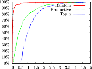
(c) $C_{S}$ (* 10000)

(d) $C_{S}$ (* 10000)

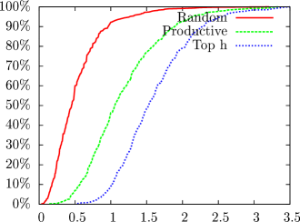
(e) $m$

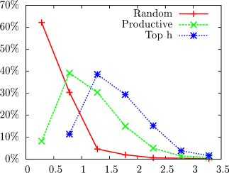
(f) $m$

(g) $p$ (* 1000)

(h) $p$ (* 1000)

Figure 5: Distributions of h-index, $m$, $p$, $C_{S}$ (left, cummulative)

We have conducted further experiments to study the behavior of other common factors like $\alpha$ [5] and $e^{2}$ [9]. However, the results did not show to carry any additional noticeable information, and, thus, figures for these factors are not included here.

3.3 Do we need new Indices?

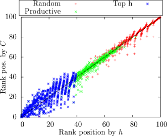
(a) $h$ vs. $C_{S}$ (unioned)

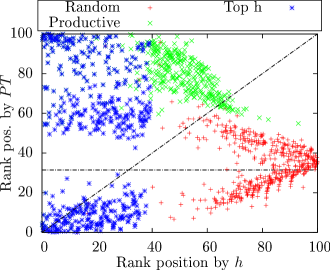
(b) $h$ vs. $PT$ (unioned)

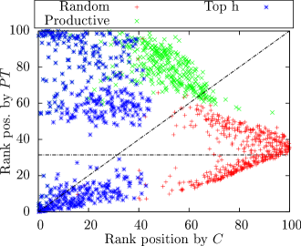
(c) $C_{S}$ vs. $PT$ (unioned)

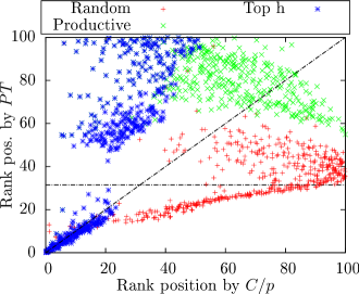
(d) $cit/p$ vs. $PT$ (unioned)

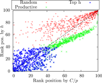
(e) $cit/p$ vs. $h$ (unioned)

Figure 6: Q-Q plots: X- and Y-axis denote normalized rank positions (%)

In this section we perform some comparisons to show that our newly defined indices differ from existing ones. Actually our new metrics separates the rank tables into two parts independently from the rank positions.

In Figure 6(a) the x-axis denotes the rank position (normalized percentagewise) of an author by h-index, whereas the y-axis denotes the rank position by the total number of citations ($C$). Each point denotes the positions of an author ranked by the two metrics. Note, that all three samples are merged but if the point is blue, then the author belongs to the "Top h" sample, if the point is green then he belongs to "Productive" sample etc. If an author belongs to more than one sample, then only one color is visible since the bullet overwrites the previous one. From Figure 6(a) the outcomes are:

• "Top h" authors are ranked in the first 40% of the rank table by h-index, as well as in the top 40% by the total number of citations ($C$).

• "Productive" authors are mainly ranked by h-index between 30% and 70%. The rank positions by $C$ are between 20% and 70%.

• "Random" authors are mainly ranked below 60% for both metrics with some outliers in the range 0-60%, mostly by $C$.

All the above remarks may seem expected for both h-index and $C$ ranking. Also, it comes out that the h-index ranking does not differ significantly from the $C$ ranking; i.e. they are correlated.

In Figure 6(b) the h-index ranking is compared to $PT$ ranking. It can be seen that there is no obvious correlation between $PT$ and h-index. Note that the horizontal line at about 32% (also, later shown in Table 5) shows the cut point of $PT$ for the zero value. Authors that reside below this line have $PT>0$ and authors above this line have $PT<0$.

• "Top h" authors are split to two groups. The first group is ranked in the top 20% of the $PT$ rank table. The second group is ranked in the last 50%. These two groups are also separated by the zero line of $PT$.

• "Productive" authors are almost all ranked at lower positions by $PT$ than by h-index. Almost all points reside above the $PT$ zero line and also above the line $y=x$ (with some exceptions at about 65-70% of the rank list).

• "Random" authors are also generally higher ranked by $PT$ than by h-index. They are also split into two groups by the line $PT=0$.

From all these statements, it seems that $PT$ is not correlated to h-index, whereas the line $PT=0$ plays the role of a symmetric axis. Thus, it emerges as the key value that separates the "Influential" authors from the "Mass producers".

Also, in Figure 6(c) we compare $PT$ ranking against $C$ (total number of citations) ranking. It is expected that the plot would be similar to Figure 6(b) based on the similarity of h-index with $C$.

In Figures 6(d) and 6(e) we compare h-index and $PT$ with the average number of citations per publication ($cit/p$) ranking. It is apparent that $PT$ is not correlated to $cit/p$. h-index is also uncorrelated to $cit/p$, however the points of the qq-plot in Figure 6(e) are closer to the line $x=y$ than the points of Figure 6(d).

Conclusively, the $PT$ ranking is not correlated to h-index, $C$ and $cit/p$. Similar graphs were produced from additional experimental comparisons that we have performed. Therefore, for brevity we do not include these graphs in this report.

3.4 Statistical Analysis

Figure 7 shows the distributions for the areas defined in the previous. In particular, Figures 7(a) and 7(b) illustrate the distributions for the $C_{T}$ (tail) area. It seems that the "Top h" cumulative distribution is very similar to the "Productive" one, however, the "Top h" distribution has slightly higher values.

Figures 7(c) and 7(d) illustrate the distributions for the $C_{TC}$ (tail complement) area. It seems that $C_{TC}$ has the same distribution as $C_{T}$ for all samples except for the sample "Productive". For latter sample $C_{TC}$ has slightly higher values than $C_{T}$. Note, also, that the "Productive" distribution has lower values for h-index than "Top h". This means that the height of the $C_{TC}$ areas is smaller for the "Productive" authors than for "Top H’ ones. The previous remarks two lead us to the (rather expected) conclusion that the "Productive" authors have long and slim tails.

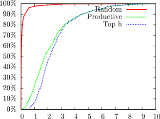
(a) $C_{T}$ (* 1000)

(b) $C_{T}$ (* 1000)

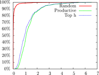
(c) $C_{TC}$ (* 10000)

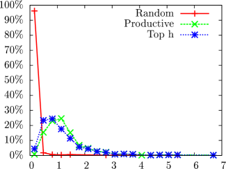
(d) $C_{TC}$ (* 10000)

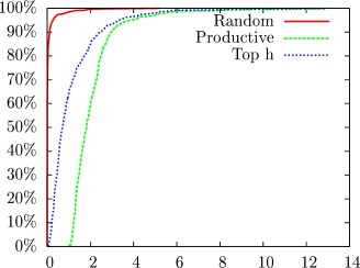
(e) $C_{IC}$ (* 100000)

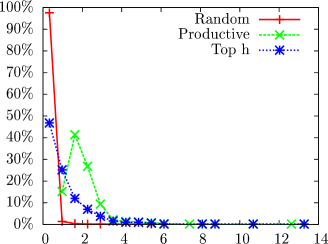
(f) $C_{IC}$ (* 100000)

Figure 7: Distributions of $C_{T}$, $C_{TC}$ (tail complement), $C_{IC}$ (ideal complement)

$C_{IC}$ distribution is shown in Figures 7(e) and 7(f). In these plots, it is clear that the "Productive" authors have clearly higher values than any other sample since $C_{I}C$ is strongly related with the total number of publications.

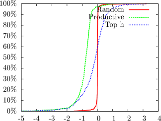
(a) $PT$ (* 10000)

(b) $PT$ (* 10000)

(c) $PT_{(\kappa=2)}$ (* 10000)

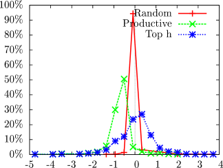
(d) $PT_{(\kappa=2)}$ (* 10000)

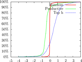
(e) $PT_{\kappa=4}$ (* 10000)

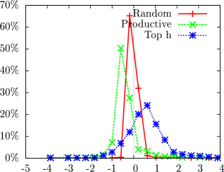
(f) $PT_{\kappa=4}$ (* 10000)

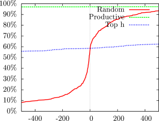
(g) $PT$ (limited x range)

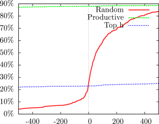
(h) $PT_{\kappa=4}$ (limited x range)

Figure 8: Distributions of $PT$, $PT_{(\kappa=2)}$ and $PT_{(\kappa=4)}$

(a) $PI$ (* 100000)

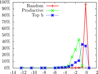
(b) $PI$ (* 100000)

(c) $PI$ (limited x range)

Figure 9: Distributions of $PI$

In Figure 8 we see the distributions for the previously defined $PT$ index. Interestingly, it seems that the value 0 is a key value. For all plots, the zero y-axis is the center of the figure. As seen in Figures 8(a) and 8(b) most of the authors are located around zero. Note that in the right plots, a point at $x=0,y=95\%$ with a previous xtic at $x=-3000$ means that the 95% of the authors have values between in the range -1500..1500. The first two plots show that the "Top h" authors have the highest values for $PT$ (about 10% of them have values greater than 8000).

Figure  8(g) is a zoomed version of Figure 8(a). In this figure, it is clear that about 96% of the "Productive" authors have $PT<0$. This means that in this sample there are a lot of "mass producers" (people with high number of publications but relatively low h-index- or at least not in "Top h-indexers"). The other samples cut the zero y-axis at about 50% to 60%, which means that 40% to 50% are positive. It is also noticeable that about 70% (15-85%) of the "Random sample have values very close to zero within the range -200..200.

In the Figure (8(c), 8(d), 8(e) and 8(f)) we also present the distributions for $PT_{\kappa=2}$ and $PT_{\kappa=4}$. We remind that factor $\kappa$ is the core area multiplier. In these plots, it is shown that these distributions behave like the basic $PT$ distribution except that they are slightly shifted to the right. The "Top h" sample is affected more than the others. This outcome is understood since they are the authors with the greatest h-index values; in other words, they have the greatest h-index core areas.

Comparing subfigure 8(h) to 8(g) we can better visualize the differences. The number of authors in the negative side of samples "Random" and "Productive" have been decreased from 70% to 25%, meaning that 45% of the sample members moved from the negative to the positive side. The number of "Productive" authors in the negative side has been decreased from 95% to 80%, i.e. an additional 15% of the sample members moved to the positive side.

In addition to the distribution plots, Table 5 presents the number of authors that have the mentioned metrics below or above zero for each sample. As mentioned before, 97% of the "Productive" authors have $PT<0$, whereas only 3% reside in the positive side of the plot. This amount increases as we increase the core factor $\kappa$. For $\kappa=4$ the increment is 17% (21% from 4%). In all other samples the increment is greater, i.e. for "Top h" the increment is 33%, for "Random" is 31%.

In Figure 9 the same kind of plots are presented for the metric $PI$. The difference is, as expected, that most of the authors lie in the negative side of the graph. The cut points of y-axis are also presented in Table 5. About 2% of the "Top h-index " authors have $PI>0$ but none of the "Productive" authors. The cut point for "Random" authors is at 6%. Also, at this point we repeat the experiment of varying the $\kappa$ value. The results do not match with those of $PT$ case. Incrementing $\kappa$ does not increase the number of positive authors in the same way as the $PT$ case. The increment is negligible for the "Productive" and "Top h" and very small for the sample "Random". This leads to the conclusion that varying the $\kappa$ factor does not affect $PI$ significantly. Probably different default values for the factors of Equation 10 (especially for $\kappa$ and/or $\iota$ ) may be needed for tuning the $PI$ metric. However, this task remains out of the scope of the present article.

Sample|	$PT$		$PT_{\kappa=2}$		$PT_{\kappa=4}$		$PI$		$PI_{\kappa=2}$		$PI_{\kappa=4}$
	$<0$	$\geq 0$	$<0$	$\geq 0$	$<0$	$\geq 0$	$<0$	$\geq 0$	$<0$	$\geq 0$	$<0$	$\geq 0$
Random	284	216	213	287	122	378	418	82	408	92	383	117
	57%	43%	43%	57%	24%	76%	84%	16%	82%	18%	77%	23%
Productive	485	15	474	26	439	61	500	0	500	0	500	0
	97%	3%	95%	5%	88%	12%	100%	0%	100%	0%	100%	0%
Top $h$	292	208	226	274	114	386	488	12	484	16	473	27
	58%	42%	45%	55%	23%	77%	98%	2%	97%	3%	95%	5%
Unioned	904	419	767	556	563	760	1230	93	1216	107	1180	143
	68%	32%	58%	42%	43%	57%	93%	7%	92%	8%	89%	11%

Table 5: $PT$ and $PI$ statistics

3.5 $PT$ robustness to self-citations

We performed another parallel experiment to study the behavior of the new metrics with respect to self-citations. A citation is considered as self if there is at least one common author between the citing and the cited paper. In Figure 10(a) a qq-plot is shown, which compares the ranking produced by h-index. The x-axis represents the rank produced by the computed h-index including self-citations, whereas y-axis represents the rank of h-index after excluding self-citations. We have performed several experiments with different types of ranking and they all show similar behavior with respect to h-index.

In Figure 10(b) the same kind of qq-plot for the $PT$ as a rank criterion is displayed. It is apparent that $PT$ is much less affected by self-citations than the h-index. This is another advantage of our new metrics; they are not affected by self-citations as other metrics and, thus, someone can rely more safely on them.

(a) $h$ vs. $h$(no-self)

(b) $PT$ vs. $PT$(no-self)

Figure 10: Q-Q plots: X and Y axis denote the rank position normalized in percent.

4 Rank Results

In this section we present some rank tables produced by using our data extracted from MAS. Table 6 shows the rank table for top-20 authors by h-index from all our samples. The corresponding $PT$ values are also shown, as well as their rank positions according to $PT$. It is remarkable that about half of them are characterized as "Mass Producers" as the have negative $PT$ values.

Author	$h$		$PT$		$p$	$C$	$C/p$
	val	pos	val	pos
Shenker Scott	97	1	5754	52	508	45621	89.81
Foster Ian	93	2	-15510	1287	768	47265	61.54
Garcia-molina Hector	92	3	-17423	1299	605	29773	49.21
Estrin Deborah	90	4	5348	62	479	40358	84.25
Ullman Jeffrey	86	5	11267	18	460	43431	94.42
Culler David	84	6	7552	38	386	32920	85.28
Tarjan Robert	83	7	2888	117	405	29614	73.12
Towsley Don	82	8	-31929	1318	793	26373	33.26
Kanade T.	81	9	-20753	1309	742	32788	44.19
Haussler David	81	10	10952	19	335	31526	94.11
Jain Anil	81	11	-11474	1236	590	29755	50.43
Papadimitriou Christos	80	12	-5897	968	506	28183	55.70
Katz Randy	78	13	-27820	1317	757	25142	33.21
Pentland Alex	77	14	-1242	724	509	32022	62.91
Han Jiawei	77	15	-15410	1285	653	28942	44.32
Jordan Michael	75	16	-1062	717	499	30738	61.60
Karp Richard	75	17	7231	41	377	29881	79.26
Zisserman A.	75	18	210	263	421	26160	62.14
Jennings Nick	74	19	-15718	1289	626	25130	40.14
Thrun S.	74	20	-5789	958	445	21665	48.69

Table 6: Rank table by $h$ (top-20 by h-index)

Author	$PT$		$h$		$p$	$C$	$C/p$
	val	pos	val	pos
Vapnik Vladimir	32542	1	50	171	126	36342	288.43
Rivest Ronald	29340	2	62	53	320	45336	141.68
Zadeh L.	25613	3	59	70	320	41012	128.16
Kohonen Teuvo	19880	4	51	157	160	25439	158.99
Floyd Sally	18059	5	66	38	222	28355	127.73
Kesselman Carl	17054	6	60	64	272	29774	109.46
Schapire Robert	16169	7	56	90	186	23449	126.07
Milner Robin	16019	8	54	108	202	24011	118.87
Shamir A	15926	9	53	125	213	24406	114.58
Tuecke Steven	14747	10	44	281	96	17035	177.45
Balakrishnan Hari	14444	11	72	21	272	28844	106.04
Agrawal Rakesh	14375	12	67	30	353	33537	95.01
Hinton G.	13415	13	63	45	314	29228	93.08
Aho Alfred	13048	14	50	173	193	20198	104.65
Lamport Leslie	12254	15	59	71	273	24880	91.14
Hopcroft John	12088	16	45	258	198	18973	95.82
Morris Robert	11685	17	57	81	305	25821	84.66
Ullman Jeffrey	11267	18	86	5	460	43431	94.42
Haussler David	10952	19	81	10	335	31526	94.11
Joachims T.	10767	20	41	377	134	14580	108.81

Table 7: Rank table by $PT$ (top-20 influential)

Author	$PT$		$h$		$p$	$C$	$C/p$
	val	pos	val	pos
Ikeuchi Katsushi	-18173	1303	43	327	638	7412	11.62
Thalmann D.	-18356	1304	46	249	632	8600	13.61
Reddy Sudhakar	-18369	1305	43	322	659	8119	12.32
Gao Wen	-18494	1306	26	649	907	4412	4.86
Prade Henri	-18692	1307	65	42	633	18228	28.80
Liu K.	-19063	1308	42	355	672	7397	11.01
Kanade T.	-20753	1309	81	9	742	32788	44.19
Rosenfeld Azriel	-21023	1310	59	73	707	17209	24.34
Gupta Anoop	-23959	1311	64	43	739	19241	26.04
Miller J.	-24112	1312	40	433	807	6568	8.14
Shin Kang	-24125	1313	57	85	731	14293	19.55
Schmidt Douglas	-24153	1314	56	94	729	13535	18.57
Bertino Elisa	-27058	1315	49	194	805	9986	12.40
Yu Philip	-27727	1316	63	48	789	18011	22.83
Katz Randy	-27820	1317	78	13	757	25142	33.21
Towsley Don	-31929	1318	82	8	793	26373	33.26
Kuo C.	-36848	1319	40	425	1148	7472	6.51
GERLA MARIO	-37464	1320	67	32	945	21362	22.61
Dongarra Jack	-39901	1321	67	31	982	21404	21.80
Poor H.	-40492	1322	55	100	1069	15278	14.29
Huang Thomas	-54047	1323	67	33	1172	19988	17.05

Table 8: Rank table by $PT$ (Last-20 - Top-20 Mass Producers)

It Table 7 we show the rank list ordered by $PT$; all authors have high rank position by h-index as well. For all of them it holds that $h>44$ except for one author, Kennedy James, who has h-index equal to 20. It can be seen that Kennedy James has only 35 publications but a total number of citations of 15482. Also, all authors that appear in this top-20 list have less than 350 publications, except for Ullman J. who has 460 with a total number of citations of 43431. All authors have a huge number of citations. For example, Rivest Ronald is ranked second by $PT$ with 45344 citations, as much as Shenker S. who is ranked first by h-index. This fact despite that Rivest Ronald has 321 publications, whereas Shenker S. has 508. Apparently, Rivest Ronald has a better citation curve. That is why Rivest Ronald chimps from the 63th place by h-index to the 2nd by $PT$ and overtakes Shenker who was first by h-index.

Based on the above rank tables, someone could say that $PT$ is correlated to the average number of citations per publication. Figures 6(d) and 6(e) show that this is not the case; actually h-index is much more correlated to $C/p$ than $PT$ (closer to line $x=y$).

Table 8 shows the top-20 "Mass Producers" from our samples. In this table we also present the average number of citations per paper ($C/p$ column). It can be seen that there is a big range of average values from 4 to 45 citations per publication in the top "Mass Producers".

Author	$PT$		$h$		$p$	$C$	$C/p$
	val	pos	val	pos
Agrawal Rakesh	14375	1	67	8	353	33537	95.01
Ullman Jeffrey	11267	2	86	2	460	43431	94.42
Motwani Rajeev	9349	3	69	6	271	23287	85.93
Fagin Ronald	4400	4	59	16	215	13604	63.27
Widom Jennifer	4031	5	71	4	280	18870	67.39
Florescu Daniela	3058	6	40	43	132	6738	51.05
Bernstein Philip	2917	7	52	22	279	14721	52.76
Buneman Peter	2001	8	43	39	158	6946	43.96
Hellerstein Joseph	1941	9	51	25	272	13212	48.57
Naughton J.	640	10	48	29	221	8944	40.47
Dewitt David	308	11	63	10	308	15743	51.11
Koudas Nick	58	12	35	50	168	4713	28.05
Sagiv Yehoshua	-196	13	42	40	209	6818	32.62
Chaudhuri Surajit	-278	14	41	41	239	7840	32.80
Egenhofer Max	-314	15	47	30	223	7958	35.69
Livny Miron	-597	16	61	12	310	14592	47.07
Suciu Dan	-659	17	54	19	285	11815	41.46
Papadias Dimitris	-809	18	38	47	200	5347	26.73
Lakshmanan Laks	-914	19	37	48	196	4969	25.35
Lenzerini M.	-1074	20	50	26	269	9876	36.71
Abiteboul Serge	-1111	21	59	15	321	14347	44.69
Ioannidis Yannis	-1647	22	39	46	209	4983	23.84
Sellis Timos	-2747	23	36	49	264	5461	20.69
Jagadish H.	-2924	24	52	24	303	10128	33.43
Dayal Umeshwar	-2975	25	44	34	306	8553	27.95
Maier David	-3096	26	45	32	331	9774	29.53
Wiederhold Gio	-3320	27	43	38	315	8376	26.59
Ramakrishnan Raghu	-4249	28	52	23	348	11143	32.02
Snodgrass Rick	-4293	29	41	42	297	6203	20.89
Srivastava Divesh	-4333	30	44	35	317	7679	24.22
Ceri Stefano	-4355	31	45	33	345	9145	26.51
Kriegel Hans-Peter	-5034	32	46	31	451	13596	30.15
Stonebraker M.	-5643	33	62	11	380	14073	37.03
Halevy Alon	-5858	34	71	5	392	16933	43.20
Abbadi Amr	-6906	35	39	45	361	5652	15.66
Gray Jim	-7953	36	54	18	508	16563	32.60
Faloutsos Christos	-8509	37	68	7	484	19779	40.87
Jensen Christian	-8566	38	44	37	389	6614	17.00
Agrawal Divyakant	-9199	39	40	44	433	6521	15.06
Aalst W.	-9811	40	48	28	468	10349	22.11
Weikum Gerhard	-11700	41	44	36	467	6912	14.80
Sheth Amit	-12193	42	58	17	488	12747	26.12
Carey Michael	-14606	43	60	14	488	11074	22.69
Franklin Michael	-14765	44	60	13	559	15175	27.15
Han Jiawei	-15410	45	77	3	653	28942	44.32
Jajodia Sushil	-15483	46	53	21	554	11070	19.98
Mylopoulos John	-15513	47	53	20	569	11835	20.80
Garcia-molina Hector	-17423	48	92	1	605	29773	49.21
Bertino Elisa	-27058	49	49	27	805	9986	12.40
Yu Philip	-27727	50	63	9	789	18011	22.83

Table 9: Rank table by $PT$ of sample "DataBases"

Author	$PT$		$h$		$p$	$C$	$C/p$
	val	pos	val	pos
Donoho David	7508	1	72	2	350	27524	78.64
Cox Ingemar	3464	2	41	15	210	10393	49.49
Simoncelli Eero	2619	3	47	12	227	11079	48.81
Yeo Boon-lock	2131	4	27	44	77	3481	45.21
Rui Yong	1745	5	33	32	168	6200	36.90
Jain Ramesh	1637	6	36	25	243	9089	37.40
Yeung Minerva	1490	7	24	48	66	2498	37.85
Goljan Miroslav	1401	8	28	41	64	2409	37.64
Wiegand Thomas	602	9	32	33	262	7962	30.39
Fridrich Jessica	472	10	27	45	118	2929	24.82
ELAD MICHAEL	156	11	36	26	216	6636	30.72
Naphade Milind	136	12	24	49	106	2104	19.85
Manjunath B.	-46	13	39	20	279	9314	33.38
Orchard M.	-784	14	34	30	187	4418	23.63
Wu Min	-1079	15	27	46	169	2755	16.30
Li Mingjing	-1180	16	28	42	150	2236	14.91
Zhang Ya-Qin	-2205	17	36	28	236	4995	21.17
Hauptmann Alexander	-3183	18	34	31	243	3923	16.14
Smith John	-3277	19	40	17	282	6403	22.71
Zakhor Avideh	-3468	20	38	23	268	5272	19.67
Ebrahimi Touradj	-3520	21	31	37	272	3951	14.53
MEMON NASIR	-3736	22	32	34	286	4392	15.36
Li Shipeng	-3925	23	26	47	271	2445	9.02
Hua Xian-sheng	-4252	24	24	50	285	2012	7.06
Ma Wei-ying	-4292	25	46	13	335	9002	26.87
Ortega Antonio	-4894	26	31	36	330	4375	13.26
Xiong Zixiang	-4950	27	35	29	308	4605	14.95
Bouman C	-5592	28	27	43	380	3939	10.37
Wu Xiaolin	-6332	29	31	39	337	3154	9.36
Bovik Alan	-8008	30	39	19	507	10244	20.21
Ramchandran Kannan	-8111	31	49	11	421	10117	24.03
Liu Bede	-8784	32	38	22	436	6340	14.54
Strintzis M.	-8871	33	29	40	454	3454	7.61
Chang Edward	-9099	34	31	38	448	3828	8.54
Delp Edward	-10001	35	37	24	438	4836	11.04
Chen Liang-Gee	-10311	36	32	35	478	3961	8.29
Tekalp A.	-10552	37	40	18	448	5768	12.88
Unser Michael	-10801	38	54	6	465	11393	24.50
Vetterli M.	-11139	39	63	4	547	19353	35.38
Jain Anil	-11474	40	81	1	590	29755	50.43
Katsaggelos Aggelos	-11662	41	36	27	504	5186	10.29
Wang Yao	-11705	42	39	21	484	5650	11.67
Chang Shih-Fu	-11941	43	52	7	507	11719	23.11
Nahrstedt Klara	-12286	44	52	9	492	10594	21.53
Girod Bernd	-13613	45	52	8	529	11191	21.16
Pitas Ioannis	-13849	46	44	14	515	6875	13.35
Chellappa Rama	-14092	47	50	10	604	13608	22.53
Zhang Hongjiang	-15112	48	63	5	556	15947	28.68
Kuo C.	-36848	49	40	16	1148	7472	6.51
Huang Thomas	-54047	50	67	3	1172	19988	17.05

Table 10: Rank table by $PT$ of sample "Multimedia"

Author	$PT$		$h$		$p$	$C$	$C/p$
	val	pos	val	pos
Jacobson Van	19982	1	44	44	161	25130	156.09
Floyd Sally	18059	2	66	9	222	28355	127.73
Balakrishnan Hari	14444	3	72	7	272	28844	106.04
Johnson David	12180	4	54	21	263	23466	89.22
Morris Robert	11685	5	57	16	305	25821	84.66
Handley M.	10763	6	47	35	201	18001	89.56
Perkins C.	9609	7	52	25	373	26301	70.51
Paxson Vern	8871	8	60	12	233	19251	82.62
Stoica Ion	8558	9	63	11	266	21347	80.25
Heidemann John	8059	10	47	36	237	16989	71.68
Culler David	7552	11	84	3	386	32920	85.28
Shenker Scott	5754	12	97	1	508	45621	89.81
Govindan Ramesh	5356	13	55	19	287	18116	63.12
Estrin Deborah	5348	14	90	2	479	40358	84.25
Crovella Mark	4886	15	46	38	172	10682	62.10
Perrig Adrian	4304	16	58	14	247	15266	61.81
Lu Songwu	3430	17	44	45	129	7170	55.58
Akyildiz Ian	3089	18	53	23	401	21533	53.70
Kleinrock Leonard	1986	19	51	31	282	13767	48.82
Knightly Edward	263	20	41	50	172	5634	32.76
Peterson L.	-652	21	54	22	292	12200	41.78
Hubaux Jean-Pierre	-653	22	45	43	247	8437	34.16
Vaidya Nitin	-1242	23	50	32	337	13108	38.90
Zhang Lixia	-1609	24	55	20	374	15936	42.61
Low Steven	-1796	25	45	42	291	9274	31.87
Boudec Jean-Yves	-2338	26	44	46	258	7078	27.43
Win Moe	-2619	27	46	37	341	10951	32.11
Rexford Jennifer	-2632	28	49	33	269	8148	30.29
Zhang Hui	-3344	29	52	27	352	12256	34.82
Srikant R.	-3827	30	46	39	328	9145	27.88
Diot Christophe	-4054	31	52	30	290	8322	28.70
Simon Marvin	-4450	32	42	49	370	9326	25.21
Ammar Mostafa	-4547	33	43	48	308	6848	22.23
Kurose Jim	-5114	34	59	13	391	14474	37.02
Campbell Andrew	-6036	35	46	41	348	7856	22.57
Chlamtac I.	-6274	36	43	47	357	7228	20.25
Crowcroft Jon	-6863	37	48	34	404	10225	25.31
WHITT W.	-7759	38	52	29	394	10025	25.44
Goldsmith A.	-7819	39	57	17	479	16235	33.89
Srivastava Mani	-8139	40	57	18	423	12723	30.08
Paulraj A.	-8421	41	64	10	442	15771	35.68
Schulzrinne Henning	-11050	42	53	24	555	15556	28.03
Garcia-Luna-Aceves J.	-11169	43	46	40	460	7875	17.12
Nahrstedt Klara	-12286	44	52	28	492	10594	21.53
Cioffi J.	-14685	45	52	26	575	12511	21.76
Mukherjee B.	-15702	46	58	15	535	11964	22.36
Katz Randy	-27820	47	78	5	757	25142	33.21
Towsley Don	-31929	48	82	4	793	26373	33.26
GERLA MARIO	-37464	49	67	8	945	21362	22.61
Giannakis Georgios	-44707	50	77	6	932	21128	22.67

Table 11: Rank table by $PT$ of sample "Networks"

Tables 9,10 and 11 resent the top 50 researchers from each of the areas of Databases (Table 9), Multimedia (Table 10) and Networks (Table 11). We have re-rank then by using the $PT$ metric.

5 Conclusions & Future Work

In this article we have defined two new areas on an author’s citation curve:

• the tail complement penalty area (TC-area), i.e. the complement of the tail with respect to the rectangle $h\times(p-h)$, with size $C_{TC}$.

• the ideal complement penalty area (IC-area), i.e. a complement with respect to the square $p\times p$, with size $C_{IC}$.

By using the above areas we have defined two new metrics:

• the penalty index based on the TC-area, in short $PT$ index, and

• the penalty index based on the IC-area, in short $PI$ index.

We have performed several experiments to study the behavior of the $PT$ and $PI$ indices. For this purpose, we have generated 3 datasets (with random authors, with prolific authors and with authors with high h-index) by extracting data from the Microsoft Academic Search database. Our contribution is threefold:

• we have shown that both new indices, $PT$ and $PI$, are un-correlated to previous ones, such as the h-index.

• we have used these new indices, in particular $PT$, to rank authors in general and, in particular, to split the population of authors into two distinct groups: the "influential" ones with $PT>0$ vs. the "mass producers" with $PT<0$. Finally,

• it has been shown that ranking authors with the $PT$ metric is more robust than the h-index with respect to noise of self-citations.

A future work will be integrate the notion of contemporary h-index [7] into the $PT$ metric.

References

- [1] L. Egghe. An improvement of the -index: The -index. ISSI Newsletter, 5, Jan. 2006.
- [2] Leo Egghe. Theory and practice of the -index. Scientometrics, 69(1):131–152, 2006.
- [3] Wikipedia. http://en.wikipedia.org/wiki/H-index.
- [4] A.W. Harzing. Publish or perish. 2007.
- [5] J. E. Hirsch. An index to quantify an individual’s scientific research output. Proceedings of the National Academy of Sciences, 102(46):16569–16572, 2005.
- [6] Michael S. Rosenberg. A biologist’s guide to impact factors. Technical report, School of Life Sciences, Arizona State University, Tempe, 2011.
- [7] Antonis Sidiropoulos, Dimitrios Katsaros, and Yannis Manolopoulos. Generalized hirsch -index for disclosing latent facts in citation networks. Scientometrics, 72(2):253–280, 2007.
- [8] Fred Ye and Ronald Rousseau. Probing the -core: an investigation of the tailcore ratio for rank distributions. Scientometrics, 84:431–439, 2010.
- [9] Chun-Ting Zhang. The -index, complementing the -index for excess citations. PLoS ONE, 4(5):e5429, May 2009.