From regional pulse vaccination to global disease eradication: insights from a mathematical model of Poliomyelitis

Cameron Browne1, Robert Smith?2, Lydia Bourouiba3
Abstract

Mass-vaccination campaigns are an important strategy in the global fight against poliomyelitis and measles. The large-scale logistics required for these mass immunisation campaigns magnifies the need for research into the effectiveness and optimal deployment of pulse vaccination. In order to better understand this control strategy, we propose a mathematical model accounting for the disease dynamics in connected regions, incorporating seasonality, environmental reservoirs and independent periodic pulse vaccination schedules in each region. The effective reproduction number, Resubscript𝑅𝑒R_{e}, is defined and proved to be a global threshold for persistence of the disease. Analytical and numerical calculations show the importance of synchronising the pulse vaccinations in connected regions and the timing of the pulses with respect to the pathogen circulation seasonality. Our results indicate that it may be crucial for mass-vaccination programs, such as national immunisation days, to be synchronised across different regions. In addition, simulations show that a migration imbalance can increase Resubscript𝑅𝑒R_{e} and alter how pulse vaccination should be optimally distributed among the patches, similar to results found with constant-rate vaccination. Furthermore, contrary to the case of constant-rate vaccination, the fraction of environmental transmission affects the value of Resubscript𝑅𝑒R_{e} when pulse vaccination is present.

1. Department of Mathematics, Vanderbilt University, Nashville TN, cameron.j.browne@vanderbilt.edu

2. Department of Mathematics and Faculty of Medicine, The University of Ottawa, Ottawa ON,
rsmith43@uottawa.ca (to whom correspondence should be addressed)

3. Department of Mathematics, Massachusetts Institute of Technology, Boston MA, lbouro@mit.edu

1 Introduction

There are three criteria for the eradication of an infectious disease: 1. biological and technical feasibility; 2. costs and benefits; and 3. societal and political considerations [3]. Despite eradication hopes for malaria, yaws and yellow fever in the twentieth century, smallpox remains the only human disease eradicated [3]. Current eradication programs include poliomyelitis (polio) [38], leprosy [19] and guinea worm disease [30]. Measles, rubella, and hepatitis A and B are also biologically and technically feasible candidates for eradication [26]. Despite strong biological, technical and cost-benefit arguments for infectious-disease eradication, securing societal and political commitments is a substantial challenge [3].

With communities more connected than ever, the control or eradication of an infectious disease requires coordinated efforts at many levels, from cities to nations. For vaccine-preventable diseases, public health authorities plan immunisation strategies across varying regions with limited resources. The World Health Organization (WHO) has helped to organise global immunisation efforts, leading to significant global reduction in polio and measles cases [38]. One vaccination strategy that has been utilised in the global fight against polio and measles is mass immunisation, which may be regarded as a pulse vaccination [10]. The complex logistics required for these mass-immunisation campaigns magnifies the need for research into the effectiveness and optimal deployment of pulse vaccination [44].

Pulse vaccination has been investigated in several mathematical models, often in disease models with seasonal transmission. Many diseases show seasonal patterns in circulation; thus inclusion of seasonality may be crucial. Agur et al. (1993) argued for pulse vaccination using a model of seasonal measles transmission, conjecturing that the pulses may antagonise the periodic disease dynamics and achieve control at a reduced cost of vaccination [2]. Shulgin et al. (1998) investigated the local stability of the disease-free periodic solution in a seasonally forced population model with three groups: susceptible (S), infected (I) and recovered (R). They considered pulse vaccination and explicitly found the threshold pulsing period [32]. Recently, Onyango and Müller considered optimal periodic vaccination strategies in the seasonally forced SIR model and found that a well-timed pulse is optimal, but its effectiveness is often close to that of constant-rate vaccination [29].

In addition to seasonality, spatial structure has been recognised as an important factor for disease dynamics and control [39]. Heterogeneity in the population movement, along with the patchy distribution of populations, suggests the use of metapopulation models describing disease transmission in patches or spatially structured populations or regions. Mobility can be incorporated and tracked in these models in various forms. Common models include linear constant fluxes representing long-term population motion (e.g. migration [22]) and nonlinear mass-action representing short-term mobility [24]. Liu et al. (2009) and Burton et al. (2012) considered epidemic models with both types of movement [14, 23]. A possible inherent advantage of pulse vaccination in a spatially structured setting, discussed by Earn et al. (1998), is that the disease dynamics in coupled regions can become synchronised by pulse vaccination, thereby increasing the probability of global disease eradication [16]. Earn et al. presented simulations of patch synchronisation after simultaneous pulse vaccinations in a seasonal SEIR metapopulation model in which the patch population dynamics were initially out of phase. Here an additional population class of Exposed (E) was considered.

Coordinating simultaneous pulse vaccination campaigns in connected regions may be vital for successful employment of pulse-vaccination strategies. Indeed, employing synchronised pulse vaccinations across large areas in the form of National Immunisation Days (NIDs) and, on an international scale, with simultaneous NIDs, has been successful in fighting polio [10]. An example of large-scale coordination among nations is Operation MECACAR (the coordinated poliomyelitis eradication efforts in Mediterranean, Caucasus and central Asian republics), which were initiated in 1995. The project was viewed as a success and an illustration of international coordination in disease control [37]. However, public health, including the control of infectious diseases and epidemics, has usually been managed on a national or regional scale, despite the potential impact of population movement [37].

Recently, pulse vaccination has been analysed in epidemic metapopulation models [33, 42]. Terry (2010) [33] presented a sufficient condition for eradication in an SIR patch model with periodic pulse vaccinations independently administered in each patch with linear migration rates, but left open the problem of finding a threshold quantity for eradication and evaluating the effect of pulse synchronisation and seasonality. Yang and Xiao (2010) [42] conducted a global analysis of an SIR patch model with synchronous periodic pulse vaccinations and linear migration rates; however, they did not allow for the different patches to administer the pulses at distinct times and seasons.

A major poliovirus transmission route in Africa and the Middle East is fecal-to-oral transmission. In this indirect route, often facilitated by inadequate water management, water plays an analogous role to that of a reservoir, although such an environmental reservoir does not allow the pathogen to reproduce. Nevertheless, its effect on the pathogen dispersal can dramatically modify epidemic patterns [11, 12]. The competition between the direct and indirect transmission routes was examined in the case of highly pathogenic avian influenza H5N1 [12], showing that indirect fecal-to-oral transmission could lead to a higher death toll than that associated with direct contact transmission.

In this article, we consider an SIR metapopulation model with both short- and long-term mobility, direct and indirect (environmental) transmission, seasonality and independent periodic pulse vaccination in each patch. The primary objectives are to find the effective reproduction number, Resubscript𝑅𝑒R_{e}, prove that it provides a sharp eradication threshold and assess the optimal timing of pulse vaccinations in the sense of minimising Resubscript𝑅𝑒R_{e}. Our mathematical model and analysis allow us to evaluate how pulse synchronisation across connected patches affects the efficacy of the overall pulse-vaccination strategy. We also determine how different movement scenarios affect the optimal deployment of vaccinations across the patches, along with considering how environmental transmission affects results. Finally, we discuss how pulse vaccination and constant-rate vaccination strategies compare when considering the goal of poliomyelitis global eradication.

This paper is organised as follows. In Section 2, we describe and give motivation for the mathematical model. In Section 3, we analyse the disease-free system, which is necessary to characterise the dynamics of the model. In Section 4, Resubscript𝑅𝑒R_{e} is defined. In Section 5, we prove that if Re<1subscript𝑅𝑒1R_{e}<1, the disease dies out, and if Re>1subscript𝑅𝑒1R_{e}>1, then it is uniformly persistent. In Section 6, we consider a two-patch example, which provides insight into the optimal timing of pulse vaccinations, the effect of mobility and environmental transmission parameters on Resubscript𝑅𝑒R_{e}, and a comparison of pulse vaccination to constant-rate vaccination in this setting. In this section, we also prove that pulse synchronization is optimal for a special case of the model and provide numerical simulations to illustrate this result in more general settings. Finally, in Section 7, we provide a discussion of the implications of our results and future work to consider.

2 The mathematical model

We consider a variant of an SIR metapopulation model with N𝑁N patches, each with populations of susceptible, infected and recovered denoted by Sjsubscript𝑆𝑗S_{j}, Ijsubscript𝐼𝑗I_{j} and Rjsubscript𝑅𝑗R_{j} for each patch 1jN1𝑗𝑁1\leq j\leq N. All three groups migrate from patch j𝑗j to patch i𝑖i, ij𝑖𝑗i\neq j, at the rates mijSjsubscript𝑚𝑖𝑗subscript𝑆𝑗m_{ij}S_{j}, kijIjsubscript𝑘𝑖𝑗subscript𝐼𝑗k_{ij}I_{j} and lijRjsubscript𝑙𝑖𝑗subscript𝑅𝑗l_{ij}R_{j}. The per capita rates at which susceptible, infected and recovered leave patch i𝑖i are mii=jimjisubscript𝑚𝑖𝑖subscript𝑗𝑖subscript𝑚𝑗𝑖m_{ii}=-\sum_{j\neq i}m_{ji}, kii=jikjisubscript𝑘𝑖𝑖subscript𝑗𝑖subscript𝑘𝑗𝑖k_{ii}=-\sum_{j\neq i}k_{ji} and lii=jiljisubscript𝑙𝑖𝑖subscript𝑗𝑖subscript𝑙𝑗𝑖l_{ii}=-\sum_{j\neq i}l_{ji}, respectively. The effect of short-term mobility on infection dynamics is modelled by mass-action coupling terms; for example, βij(t)IjSisubscript𝛽𝑖𝑗𝑡subscript𝐼𝑗subscript𝑆𝑖\beta_{ij}(t)I_{j}S_{i}. For this infection rate, infected individuals from patch j𝑗j are assumed to travel to patch i𝑖i, infect some susceptibles in patch i𝑖i and then return to patch j𝑗j on a shorter timescale than that of the disease dynamics. Conversely, susceptibles from patch i𝑖i can travel to patch j𝑗j, become infected and return to patch i𝑖i on the shorter timescale.

In the model for poliomyelitis presented herein, both direct contact and indirect environmental routes are considered. The environmental contamination of the virus in each patch j𝑗j is described by a state variable, denoted by Gjsubscript𝐺𝑗G_{j}. Infected individuals in patch j𝑗j (Ijsubscript𝐼𝑗I_{j}) shed the virus into the environmental reservoir Gjsubscript𝐺𝑗G_{j} at the rate ξj(t)Ijsubscript𝜉𝑗𝑡subscript𝐼𝑗\xi_{j}(t)I_{j}. The virus in the environmental reservoir cannot reproduce outside of the host and decays at the rate νj(t)Gjsubscript𝜈𝑗𝑡subscript𝐺𝑗\nu_{j}(t)G_{j}. The virus in the environmental reservoir j𝑗j, Gjsubscript𝐺𝑗G_{j}, contributes to the infected population in patch Iisubscript𝐼𝑖I_{i} through the mass-action term ϵij(t)SiGjsubscriptitalic-ϵ𝑖𝑗𝑡subscript𝑆𝑖subscript𝐺𝑗\epsilon_{ij}(t)S_{i}G_{j}. Direct transmission contributing to Iisubscript𝐼𝑖I_{i} is represented by the mass-action term Sijβij(t)Ijsubscript𝑆𝑖subscript𝑗subscript𝛽𝑖𝑗𝑡subscript𝐼𝑗S_{i}\sum_{j}\beta_{ij}(t)I_{j}. Due to possible seasonality of poliovirus circulation [38], both direct and environmental transmission parameters βij(t)subscript𝛽𝑖𝑗𝑡\beta_{ij}(t), ϵij(t)subscriptitalic-ϵ𝑖𝑗𝑡\epsilon_{ij}(t), ξi(t)subscript𝜉𝑖𝑡\xi_{i}(t) and νi(t)subscript𝜈𝑖𝑡\nu_{i}(t) are assumed to be periodic with a period of one year.

Pulse vaccination is modelled through impulses on the system occurring at fixed times. First, we consider a general pulse vaccination scheme with no periodicity. For each patch i𝑖i, pulse vaccinations occur at times ti,nsubscript𝑡𝑖𝑛t_{i,n} where n=1,2,𝑛12n=1,2,\dots At time ti,nsubscript𝑡𝑖𝑛t_{i,n}, a fraction ψi,nsubscript𝜓𝑖𝑛\psi_{i,n} of the susceptible population Sisubscript𝑆𝑖S_{i} is instantly immunised and transferred to the recovered class Risubscript𝑅𝑖R_{i}. Therefore Si((ti,n)+)=(1ψi,n)Si((ti,n))subscript𝑆𝑖superscriptsubscript𝑡𝑖𝑛1subscript𝜓𝑖𝑛subscript𝑆𝑖superscriptsubscript𝑡𝑖𝑛S_{i}\left((t_{i,n})^{+}\right)=\left(1-\psi_{i,n}\right)S_{i}\left((t_{i,n})^{-}\right) and Ri((ti,n)+)=ψi,nSi((ti,n))subscript𝑅𝑖superscriptsubscript𝑡𝑖𝑛subscript𝜓𝑖𝑛subscript𝑆𝑖superscriptsubscript𝑡𝑖𝑛R_{i}\left((t_{i,n})^{+}\right)=\psi_{i,n}S_{i}\left((t_{i,n})^{-}\right), where Si((ti,n)+)subscript𝑆𝑖superscriptsubscript𝑡𝑖𝑛S_{i}\left((t_{i,n})^{+}\right) and Si((ti,n))subscript𝑆𝑖superscriptsubscript𝑡𝑖𝑛S_{i}\left((t_{i,n})^{-}\right) denote limits from the right-hand side and left-hand side, respectively.

For each patch i𝑖i, demography is modeled with constant birth rate, bisubscript𝑏𝑖b_{i}, into the susceptible class and a per capita death rate, μisubscript𝜇𝑖\mu_{i}. The parameter pisubscript𝑝𝑖p_{i} represents the fraction of newborns who are successfully vaccinated. The parameter γisubscript𝛾𝑖\gamma_{i} is the recovery rate. Note that both recovery from infection and successful vaccination induce perfect life-long immunity. All parameters are assumed to be non-negative, and the parameters νi(t)subscript𝜈𝑖𝑡\nu_{i}(t), μisubscript𝜇𝑖\mu_{i} and bisubscript𝑏𝑖b_{i} are additionally assumed to be positive. We thus arrive at the following mathematical model:

dSidt𝑑subscript𝑆𝑖𝑑𝑡\displaystyle\frac{dS_{i}}{dt} =(1pi)biμiSiSijβij(t)IjSijϵij(t)Gj+jmijSjabsent1subscript𝑝𝑖subscript𝑏𝑖subscript𝜇𝑖subscript𝑆𝑖subscript𝑆𝑖subscript𝑗subscript𝛽𝑖𝑗𝑡subscript𝐼𝑗subscript𝑆𝑖subscript𝑗subscriptitalic-ϵ𝑖𝑗𝑡subscript𝐺𝑗subscript𝑗subscript𝑚𝑖𝑗subscript𝑆𝑗\displaystyle=(1-p_{i})b_{i}-\mu_{i}S_{i}-S_{i}\sum_{j}\beta_{ij}(t)I_{j}-S_{i}\sum_{j}\epsilon_{ij}(t)G_{j}+\sum_{j}m_{ij}S_{j} t𝑡\displaystyle t ti,nabsentsubscript𝑡𝑖𝑛\displaystyle\neq t_{i,n} (1)
dIidt𝑑subscript𝐼𝑖𝑑𝑡\displaystyle\frac{dI_{i}}{dt} =Sijβij(t)Ij+Sijϵij(t)Gj(μi+γi)Ii+jkijIjabsentsubscript𝑆𝑖subscript𝑗subscript𝛽𝑖𝑗𝑡subscript𝐼𝑗subscript𝑆𝑖subscript𝑗subscriptitalic-ϵ𝑖𝑗𝑡subscript𝐺𝑗subscript𝜇𝑖subscript𝛾𝑖subscript𝐼𝑖subscript𝑗subscript𝑘𝑖𝑗subscript𝐼𝑗\displaystyle=S_{i}\sum_{j}\beta_{ij}(t)I_{j}+S_{i}\sum_{j}\epsilon_{ij}(t)G_{j}-(\mu_{i}+\gamma_{i})I_{i}+\sum_{j}k_{ij}I_{j} t𝑡\displaystyle t ti,nabsentsubscript𝑡𝑖𝑛\displaystyle\neq t_{i,n}
dGidt𝑑subscript𝐺𝑖𝑑𝑡\displaystyle\frac{dG_{i}}{dt} =ξi(t)Iiνi(t)Giabsentsubscript𝜉𝑖𝑡subscript𝐼𝑖subscript𝜈𝑖𝑡subscript𝐺𝑖\displaystyle=\xi_{i}(t)I_{i}-\nu_{i}(t)G_{i}\phantom{+S_{i}\sum_{j}\epsilon_{ij}(t)G_{j}} t𝑡\displaystyle t ti,nabsentsubscript𝑡𝑖𝑛\displaystyle\neq t_{i,n}
dRidt𝑑subscript𝑅𝑖𝑑𝑡\displaystyle\frac{dR_{i}}{dt} =pibi+γiIiμiRi+jlijRjabsentsubscript𝑝𝑖subscript𝑏𝑖subscript𝛾𝑖subscript𝐼𝑖subscript𝜇𝑖subscript𝑅𝑖subscript𝑗subscript𝑙𝑖𝑗subscript𝑅𝑗\displaystyle=p_{i}b_{i}+\gamma_{i}I_{i}-\mu_{i}R_{i}+\sum_{j}l_{ij}R_{j} t𝑡\displaystyle t ti,nabsentsubscript𝑡𝑖𝑛\displaystyle\neq t_{i,n}
Si(ti,n+)subscript𝑆𝑖superscriptsubscript𝑡𝑖𝑛\displaystyle S_{i}\left(t_{i,n}^{+}\right) =(1ψi,n)Si(ti,n)absent1subscript𝜓𝑖𝑛subscript𝑆𝑖superscriptsubscript𝑡𝑖𝑛\displaystyle=\left(1-\psi_{i,n}\right)S_{i}\left(t_{i,n}^{-}\right) t𝑡\displaystyle t =ti,nabsentsubscript𝑡𝑖𝑛\displaystyle=t_{i,n}
Ri(ti,n+)subscript𝑅𝑖superscriptsubscript𝑡𝑖𝑛\displaystyle R_{i}\left(t_{i,n}^{+}\right) =ψi,nSi(ti,n)absentsubscript𝜓𝑖𝑛subscript𝑆𝑖superscriptsubscript𝑡𝑖𝑛\displaystyle=\psi_{i,n}S_{i}\left(t_{i,n}^{-}\right) t𝑡\displaystyle t =ti,n.absentsubscript𝑡𝑖𝑛\displaystyle=t_{i,n}.

Consider the non-negative cone of 4Nsuperscript4𝑁\mathbb{R}^{4N}, denoted by X=+4N𝑋subscriptsuperscript4𝑁X=\mathbb{R}^{4N}_{+}. The following theorem shows existence and uniqueness of solutions to (1), the invariance of +4Nsubscriptsuperscript4𝑁\mathbb{R}^{4N}_{+} and ultimate uniform boundedness of solutions.

Theorem 1.

For any initial condition x0+4Nsubscript𝑥0subscriptsuperscript4𝑁x_{0}\in\mathbb{R}^{4N}_{+}, there exists a unique solution to system (1), φ(t,x0)𝜑𝑡subscript𝑥0\varphi(t,x_{0}), which is smooth for all tti,n𝑡subscript𝑡𝑖𝑛t\neq t_{i,n} and the flow φ(t,x)𝜑𝑡𝑥\varphi(t,x) is continuous with respect to initial condition x𝑥x. Moreover, the non-negative quadrant +4Nsubscriptsuperscript4𝑁\mathbb{R}^{4N}_{+} is invariant and there exists M>0𝑀0M>0 such that lim suptφ(t,x)Msubscriptlimit-supremum𝑡norm𝜑𝑡𝑥𝑀\limsup_{t\rightarrow\infty}\left\|\varphi(t,x)\right\|\leq M for all x+4N𝑥subscriptsuperscript4𝑁x\in\mathbb{R}^{4N}_{+}.

Proof.

The existence, uniqueness, and regularity for non-impulse times come from results that can be found in [25]. In order to show the invariance of +4Nsubscriptsuperscript4𝑁\mathbb{R}^{4N}_{+}, consider the set Y0{x+4N:xi=0,N+1i3N}superscript𝑌0conditional-set𝑥subscriptsuperscript4𝑁formulae-sequencesubscript𝑥𝑖0𝑁1𝑖3𝑁\partial Y^{0}\equiv\left\{x\in\mathbb{R}^{4N}_{+}:x_{i}=0,\ N+1\leq i\leq 3N\right\}. On this set, dIidt=dGidt=0𝑑subscript𝐼𝑖𝑑𝑡𝑑subscript𝐺𝑖𝑑𝑡0\frac{dI_{i}}{dt}=\frac{dG_{i}}{dt}=0, so Y0superscript𝑌0\partial Y^{0} is invariant. Also, notice that dSidt0𝑑subscript𝑆𝑖𝑑𝑡0\frac{dS_{i}}{dt}\geq 0 if Si=0subscript𝑆𝑖0S_{i}=0. Then, by uniqueness of solutions, we find that +4Nsubscriptsuperscript4𝑁\mathbb{R}^{4N}_{+} is invariant.

To show ultimate boundedness, consider the total population of individuals, Ni(Si+Ii+Ri)𝑁subscript𝑖subscript𝑆𝑖subscript𝐼𝑖subscript𝑅𝑖N\equiv\sum_{i}\left(S_{i}+I_{i}+R_{i}\right). Then, adding all the appropriate equations of (1), we obtain that

dN(t)dtbμN(t)t0,formulae-sequence𝑑𝑁𝑡𝑑𝑡𝑏𝜇𝑁𝑡for-all𝑡0\frac{dN(t)}{dt}\leq b-\mu N(t)\qquad\forall t\geq 0,

where b=max(b1,,bN)𝑏subscript𝑏1subscript𝑏𝑁b=\max(b_{1},\dots,b_{N}) and μ=min(μ1,,μN)𝜇subscript𝜇1subscript𝜇𝑁\mu=\min(\mu_{1},\dots,\mu_{N}). A simple comparison principle yields lim suptN(t)bμsubscriptlimit-supremum𝑡𝑁𝑡𝑏𝜇\limsup_{t\rightarrow\infty}N(t)\leq\frac{b}{\mu}. This implies that lim suptG(t)ξbνμsubscriptlimit-supremum𝑡𝐺𝑡𝜉𝑏𝜈𝜇\limsup_{t\rightarrow\infty}G(t)\leq\frac{\xi b}{\nu\mu} where ξ=max(ξ1,,ξn)𝜉subscript𝜉1subscript𝜉𝑛\xi=\max(\xi_{1},\dots,\xi_{n}) and ν=min(ν1,,νN)𝜈subscript𝜈1subscript𝜈𝑁\nu=\min(\nu_{1},\dots,\nu_{N}). Therefore, if φ(t,x)𝜑𝑡𝑥\varphi(t,x) denotes the family of solutions, then there exists M>0𝑀0M>0 such that lim suptφ(t,x)Msubscriptlimit-supremum𝑡norm𝜑𝑡𝑥𝑀\limsup_{t\rightarrow\infty}\left\|\varphi(t,x)\right\|\leq M for all x+4N𝑥subscriptsuperscript4𝑁x\in\mathbb{R}^{4N}_{+}. ∎

In order to analyse the asymptotic dynamics of the system, we assume some periodicity in the impulses. According to WHO guidelines, countries threatened by wild poliovirus should hold NIDs twice a year with 4–6 weeks separating the immunisation campaigns within a year [10]. Hence we consider a sufficiently flexible schedule in order to cover this guideline. Suppose that, for patch i{1,2,,N}𝑖12𝑁i\in\left\{1,2,\dots,N\right\}, the pulse vaccinations occur on a periodic schedule of period τisubscript𝜏𝑖\tau_{i}. Assume that there exists τ𝜏\tau\in\mathbb{N} such that τ=n1τ1==nNτN𝜏subscript𝑛1subscript𝜏1subscript𝑛𝑁subscript𝜏𝑁\tau=n_{1}\tau_{1}=\cdots=n_{N}\tau_{N}, where n1,,nNsubscript𝑛1subscript𝑛𝑁n_{1},\dots,n_{N}\in\mathbb{N}; i.e., there exists a common period τ𝜏\tau for pulse vaccinations among the patches. For each patch i{1,2,,N}𝑖12𝑁i\in\left\{1,2,\dots,N\right\}, we assume that there are Lisubscript𝐿𝑖L_{i} pulse vaccinations that occur within the period τisubscript𝜏𝑖\tau_{i}. More precisely, the pulse vaccinations for patch i𝑖i occur at times t=nτi+ϕik𝑡𝑛subscript𝜏𝑖superscriptsubscriptitalic-ϕ𝑖𝑘t=n\tau_{i}+\phi_{i}^{k}, where 0ϕik<τi0superscriptsubscriptitalic-ϕ𝑖𝑘subscript𝜏𝑖0\leq\phi_{i}^{k}<\tau_{i}, n𝑛n\in\mathbb{N} and k{1,..,Li}k\in\left\{1,..,L_{i}\right\}. Note that the recovered (or removed) classes are decoupled from the remaining system and can thus be neglected. We obtain the following model:

dSidt𝑑subscript𝑆𝑖𝑑𝑡\displaystyle\frac{dS_{i}}{dt} =(1pi)biμiSiSijβij(t)IjSijϵij(t)Gj+jmijSjabsent1subscript𝑝𝑖subscript𝑏𝑖subscript𝜇𝑖subscript𝑆𝑖subscript𝑆𝑖subscript𝑗subscript𝛽𝑖𝑗𝑡subscript𝐼𝑗subscript𝑆𝑖subscript𝑗subscriptitalic-ϵ𝑖𝑗𝑡subscript𝐺𝑗subscript𝑗subscript𝑚𝑖𝑗subscript𝑆𝑗\displaystyle=(1-p_{i})b_{i}-\mu_{i}S_{i}-S_{i}\sum_{j}\beta_{ij}(t)I_{j}-S_{i}\sum_{j}\epsilon_{ij}(t)G_{j}+\sum_{j}m_{ij}S_{j} t𝑡\displaystyle t nτi+ϕikabsent𝑛subscript𝜏𝑖superscriptsubscriptitalic-ϕ𝑖𝑘\displaystyle\neq n\tau_{i}+\phi_{i}^{k} (2)
dIidt𝑑subscript𝐼𝑖𝑑𝑡\displaystyle\frac{dI_{i}}{dt} =Sijβij(t)Ij+Sijϵij(t)Gj(μi+γi)Ii+jkijIjabsentsubscript𝑆𝑖subscript𝑗subscript𝛽𝑖𝑗𝑡subscript𝐼𝑗subscript𝑆𝑖subscript𝑗subscriptitalic-ϵ𝑖𝑗𝑡subscript𝐺𝑗subscript𝜇𝑖subscript𝛾𝑖subscript𝐼𝑖subscript𝑗subscript𝑘𝑖𝑗subscript𝐼𝑗\displaystyle=S_{i}\sum_{j}\beta_{ij}(t)I_{j}+S_{i}\sum_{j}\epsilon_{ij}(t)G_{j}-(\mu_{i}+\gamma_{i})I_{i}+\sum_{j}k_{ij}I_{j} t𝑡\displaystyle t nτi+ϕikabsent𝑛subscript𝜏𝑖superscriptsubscriptitalic-ϕ𝑖𝑘\displaystyle\neq n\tau_{i}+\phi_{i}^{k}
dGidt𝑑subscript𝐺𝑖𝑑𝑡\displaystyle\frac{dG_{i}}{dt} =ξi(t)Iiνi(t)Giabsentsubscript𝜉𝑖𝑡subscript𝐼𝑖subscript𝜈𝑖𝑡subscript𝐺𝑖\displaystyle=\xi_{i}(t)I_{i}-\nu_{i}(t)G_{i} t𝑡\displaystyle t nτi+ϕikabsent𝑛subscript𝜏𝑖superscriptsubscriptitalic-ϕ𝑖𝑘\displaystyle\neq n\tau_{i}+\phi_{i}^{k}
Si((nτi+ϕik)+)subscript𝑆𝑖superscript𝑛subscript𝜏𝑖superscriptsubscriptitalic-ϕ𝑖𝑘\displaystyle S_{i}\left((n\tau_{i}+\phi_{i}^{k})^{+}\right) =(1ψik)Si((nτi+ϕik))absent1superscriptsubscript𝜓𝑖𝑘subscript𝑆𝑖superscript𝑛subscript𝜏𝑖superscriptsubscriptitalic-ϕ𝑖𝑘\displaystyle=\left(1-\psi_{i}^{k}\right)S_{i}\left((n\tau_{i}+\phi_{i}^{k})^{-}\right) t𝑡\displaystyle t =nτi+ϕik.absent𝑛subscript𝜏𝑖superscriptsubscriptitalic-ϕ𝑖𝑘\displaystyle=n\tau_{i}+\phi_{i}^{k}.

Model (2) will be analysed in the ensuing sections.

3 Disease-free system

In order to obtain a reproduction number, we need to determine the dynamics of the susceptible population in the absence of infection. With this in mind, consider the following characterisation of the vaccinations. Within the time interval (0,τ]0𝜏(0,\tau], there are L1n1L2n2LNnNsubscript𝐿1subscript𝑛1subscript𝐿2subscript𝑛2subscript𝐿𝑁subscript𝑛𝑁L_{1}n_{1}\cdot L_{2}n_{2}\cdots L_{N}n_{N} impulses. Some of these impulses may occur at the same time. Let pL1n1L2n2LNnN𝑝subscript𝐿1subscript𝑛1subscript𝐿2subscript𝑛2subscript𝐿𝑁subscript𝑛𝑁p\leq L_{1}n_{1}\cdot L_{2}n_{2}\cdots L_{N}n_{N} be the number of distinct impulse times. We label these impulse times in increasing order as follows: 0=t0t1<t2<<tp<tp+1=τ0subscript𝑡0subscript𝑡1subscript𝑡2subscript𝑡𝑝subscript𝑡𝑝1𝜏0=t_{0}\leq t_{1}<t_{2}<\cdots<t_{p}<t_{p+1}=\tau. For 1iN1𝑖𝑁1\leq i\leq N and 1p1𝑝1\leq\ell\leq p, let

αisuperscriptsubscript𝛼𝑖\displaystyle\alpha_{i}^{\ell} ={1ψikif t=nτi+ϕik1otherwise.absentcases1superscriptsubscript𝜓𝑖𝑘if subscript𝑡𝑛subscript𝜏𝑖superscriptsubscriptitalic-ϕ𝑖𝑘1otherwise.\displaystyle=\begin{cases}1-\psi_{i}^{k}&\text{if }t_{\ell}=n\tau_{i}+\phi_{i}^{k}\\ 1&\text{otherwise.}\end{cases}

In the absence of infection, we obtain the linear impulsive system:

dx(t)dt𝑑𝑥𝑡𝑑𝑡\displaystyle\frac{dx(t)}{dt} =Ax(t)+babsent𝐴𝑥𝑡𝑏\displaystyle=Ax(t)+b t𝑡\displaystyle t nτ+tabsent𝑛𝜏subscript𝑡\displaystyle\neq n\tau+t_{\ell} for{1,,p},nformulae-sequencefor1𝑝𝑛\displaystyle\text{for}\ \ell\in\left\{1,\dots,p\right\},n\in\mathbb{N} (3)
x((nτ+t)+)𝑥superscript𝑛𝜏subscript𝑡\displaystyle x\left((n\tau+t_{\ell})^{+}\right) =Dx((nτ+t)),absentsubscript𝐷𝑥superscript𝑛𝜏subscript𝑡\displaystyle=D_{\ell}x\left((n\tau+t_{\ell})^{-}\right),

where

x(t)𝑥𝑡\displaystyle x(t) =(x1(t)x2(t)xN(t)),A=(μ1+m11m12m1nm21μ2+m22m2nmN1mN2μN+mNN),b=((1p1)b1(1p2)b2(1pN)bN)formulae-sequenceabsentmatrixsubscript𝑥1𝑡subscript𝑥2𝑡subscript𝑥𝑁𝑡formulae-sequence𝐴matrixsubscript𝜇1subscript𝑚11subscript𝑚12subscript𝑚1𝑛subscript𝑚21subscript𝜇2subscript𝑚22subscript𝑚2𝑛subscript𝑚𝑁1subscript𝑚𝑁2subscript𝜇𝑁subscript𝑚𝑁𝑁𝑏matrix1subscript𝑝1subscript𝑏11subscript𝑝2subscript𝑏21subscript𝑝𝑁subscript𝑏𝑁\displaystyle=\begin{pmatrix}x_{1}(t)\\ x_{2}(t)\\ \vdots\\ x_{N}(t)\end{pmatrix},\qquad A=\begin{pmatrix}-\mu_{1}+m_{11}&m_{12}&\cdots&m_{1n}\\ m_{21}&-\mu_{2}+m_{22}&\cdots&m_{2n}\\ \vdots&\vdots&\ddots&\vdots\\ m_{N1}&m_{N2}&\cdots&-\mu_{N}+m_{NN}\end{pmatrix},\qquad b=\begin{pmatrix}(1-p_{1})b_{1}\\ (1-p_{2})b_{2}\\ \vdots\\ (1-p_{N})b_{N}\end{pmatrix}
Dsubscript𝐷\displaystyle D_{\ell} =diag(α1,α2,,αN),andmii=jimji.formulae-sequenceabsentdiagsuperscriptsubscript𝛼1superscriptsubscript𝛼2superscriptsubscript𝛼𝑁andsubscript𝑚𝑖𝑖subscript𝑗𝑖subscript𝑚𝑗𝑖\displaystyle={\rm diag}\left(\alpha_{1}^{\ell},\alpha_{2}^{\ell},\dots,\alpha_{N}^{\ell}\right),\qquad\text{and}\qquad m_{ii}=-\sum_{j\neq i}m_{ji}.

The solution to the linear differential equation x˙=Ax+b˙𝑥𝐴𝑥𝑏\dot{x}=Ax+b (the no-impulse version of (3)) is

θ(t,x)=etAx+(etAI)A1b,whereθ(0,x)=x.formulae-sequence𝜃𝑡𝑥superscript𝑒𝑡𝐴𝑥superscript𝑒𝑡𝐴𝐼superscript𝐴1𝑏where𝜃0𝑥𝑥\displaystyle\theta(t,x)=e^{tA}x+(e^{tA}-I)A^{-1}b,\quad\text{where}\ \ \theta(0,x)=x. (4)

We define the period map F:NN:𝐹superscript𝑁superscript𝑁F:\mathbb{R}^{N}\rightarrow\mathbb{R}^{N} for the impulsive system (3). Here F(x)=ζ(τ,x)𝐹𝑥𝜁𝜏𝑥F(x)=\zeta(\tau,x) where ζ(t,x)𝜁𝑡𝑥\zeta(t,x) is the unique solution of the impulsive system (3) with ζ(0,x)=x𝜁0𝑥𝑥\zeta(0,x)=x. The interested reader is referred to the work of Bainov and Simeonov [7, 8, 9] for more information on the theory of impulsive differential equations.

The period map, F(x)𝐹𝑥F(x), can be calculated through recursive relations. Let x0=xsubscript𝑥0𝑥x_{0}=x and iteratively calculate F(x)𝐹𝑥F(x) as follows:

xjsubscript𝑥𝑗\displaystyle x_{j} =Djθ(tjtj1,xj1)for j=1,,pformulae-sequenceabsentsubscript𝐷𝑗𝜃subscript𝑡𝑗subscript𝑡𝑗1subscript𝑥𝑗1for 𝑗1𝑝\displaystyle=D_{j}\theta(t_{j}-t_{j-1},x_{j-1})\qquad\text{for }\ j=1,\dots,p (5)
F(x)𝐹𝑥\displaystyle F(x) =θ(τtp,xp).absent𝜃𝜏subscript𝑡𝑝subscript𝑥𝑝\displaystyle=\theta(\tau-t_{p},x_{p}).

Define the following matrices Cj, 1jp+1subscript𝐶𝑗1𝑗𝑝1C_{j},\ 1\leq j\leq p+1 and C𝐶C:

Cp+1subscript𝐶𝑝1\displaystyle C_{p+1} =Iabsent𝐼\displaystyle=I
Cpsubscript𝐶𝑝\displaystyle C_{p} =e(τtp)ADpabsentsuperscript𝑒𝜏subscript𝑡𝑝𝐴subscript𝐷𝑝\displaystyle=e^{(\tau-t_{p})A}\cdot D_{p}
Cjsubscript𝐶𝑗\displaystyle C_{j} =Cj+1e(tj+1tj)ADjfor 1jp1formulae-sequenceabsentsubscript𝐶𝑗1superscript𝑒subscript𝑡𝑗1subscript𝑡𝑗𝐴subscript𝐷𝑗for 1𝑗𝑝1\displaystyle=C_{j+1}\cdot e^{(t_{j+1}-t_{j})A}\cdot D_{j}\quad\text{for }1\leq j\leq p-1
C𝐶\displaystyle C =C1et1Aabsentsubscript𝐶1superscript𝑒subscript𝑡1𝐴\displaystyle=C_{1}\cdot e^{t_{1}A}

Utilising (4) to explicitly express the recursive relations in (5), we obtain the following formula for F(x)𝐹𝑥F(x):

F(x)𝐹𝑥\displaystyle F(x) =Cx+j=1pCj+1(e(tj+1tj)AI)A1b.absent𝐶𝑥superscriptsubscript𝑗1𝑝subscript𝐶𝑗1superscript𝑒subscript𝑡𝑗1subscript𝑡𝑗𝐴𝐼superscript𝐴1𝑏\displaystyle=Cx+\sum_{j=1}^{p}C_{j+1}\left(e^{(t_{j+1}-t_{j})A}-I\right)A^{-1}b. (6)

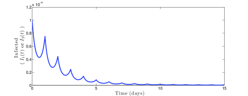
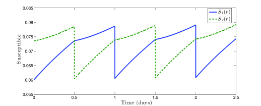
This formula will be used to explicitly calculate the periodic solution obtained in the following theorem. An example of the periodic solution is displayed in Figure 1.

Proposition 2.

The disease-free system (3) has a unique globally asymptotically stable τ𝜏\tau-periodic solution S¯(t)¯𝑆𝑡\overline{S}(t).

Proof.

A τ𝜏\tau-periodic solution of (3) corresponds to a fixed point of the period map. Hence we consider the equation x¯=F(x¯)¯𝑥𝐹¯𝑥\overline{x}=F\left(\overline{x}\right).

x¯¯𝑥\displaystyle\overline{x} =Cx¯+j=1pCj+1(e(tj+1tj)AI)A1b.absent𝐶¯𝑥superscriptsubscript𝑗1𝑝subscript𝐶𝑗1superscript𝑒subscript𝑡𝑗1subscript𝑡𝑗𝐴𝐼superscript𝐴1𝑏\displaystyle=C\overline{x}+\sum_{j=1}^{p}C_{j+1}\left(e^{(t_{j+1}-t_{j})A}-I\right)A^{-1}b.

We claim that ρ(C)<1𝜌𝐶1\rho(C)<1. To prove this claim, consider the matrix A𝐴A and define the stability modulus of A𝐴A, s(A)𝑠𝐴s(A), as s(A)max{Re(λ):λis an eigenvalue of A}𝑠𝐴:Re𝜆𝜆is an eigenvalue of 𝐴s(A)\equiv\max\left\{{\rm Re}(\lambda):\lambda\ \text{is an eigenvalue of }A\right\}. Since A𝐴A is quasi-positive, A𝐴A has an eigenvalue λ𝜆\lambda such that λ=s(A)𝜆𝑠𝐴\lambda=s(A) with an associated non-negative eigenvector v𝑣v [34]. Then w(t)=eλtv𝑤𝑡superscript𝑒𝜆𝑡𝑣w(t)=e^{\lambda t}v is a solution to x˙=Ax˙𝑥𝐴𝑥\dot{x}=Ax. Let 1=(1,1,,1)1111\vec{1}=\left(1,1,\dots,1\right) be the row vector of ones for Nsuperscript𝑁\mathbb{R}^{N}. Define u(t)=1veλt𝑢𝑡1𝑣superscript𝑒𝜆𝑡u(t)=\vec{1}ve^{\lambda t}. Then:

dudt𝑑𝑢𝑑𝑡\displaystyle\frac{du}{dt} =1(λv)eλt=1Aveλt=(μ1,μ2,,μN)veλtμ1veλt,absent1𝜆𝑣superscript𝑒𝜆𝑡1𝐴𝑣superscript𝑒𝜆𝑡subscript𝜇1subscript𝜇2subscript𝜇𝑁𝑣superscript𝑒𝜆𝑡𝜇1𝑣superscript𝑒𝜆𝑡\displaystyle=\vec{1}(\lambda v)e^{\lambda t}=\vec{1}Ave^{\lambda t}=(-\mu_{1},-\mu_{2},\dots,-\mu_{N})ve^{\lambda t}\leq-\mu\vec{1}ve^{\lambda t},

where μ=min{μi:1iN}𝜇:subscript𝜇𝑖1𝑖𝑁\mu=\min\left\{\mu_{i}:1\leq i\leq N\right\}. Thus dudt=μu(t)𝑑𝑢𝑑𝑡𝜇𝑢𝑡\frac{du}{dt}=-\mu u(t), which implies u(t)1veμt𝑢𝑡1𝑣superscript𝑒𝜇𝑡u(t)\leq\vec{1}ve^{-\mu t}. Thus λμ<0𝜆𝜇0\lambda\leq-\mu<0, so s(A)μ𝑠𝐴𝜇s(A)\leq-\mu. Therefore, by the standard theory of linear differential equations, there exists a constant K>0𝐾0K>0 such that etA<Keμtnormsuperscript𝑒𝑡𝐴𝐾superscript𝑒𝜇𝑡\left\|e^{tA}\right\|<Ke^{-\mu t}. Then

Cnnormsuperscript𝐶𝑛\displaystyle\left\|C^{n}\right\| Cnabsentsuperscriptnorm𝐶𝑛\displaystyle\leq\left\|C\right\|^{n}
(Dpe(τtp)ADp1et1A)nabsentsuperscriptnormsubscript𝐷𝑝normsuperscript𝑒𝜏subscript𝑡𝑝𝐴normsubscript𝐷𝑝1normsuperscript𝑒subscript𝑡1𝐴𝑛\displaystyle\leq\left(\left\|D_{p}\right\|||e^{(\tau-t_{p})A}||\left\|D_{p-1}\right\|\cdots\cdots\left\|e^{t_{1}A}\right\|\right)^{n}
=(e(τtp)Ai=1pe(titi1)ADi)nabsentsuperscriptnormsuperscript𝑒𝜏subscript𝑡𝑝𝐴superscriptsubscriptproduct𝑖1𝑝normsuperscript𝑒subscript𝑡𝑖subscript𝑡𝑖1𝐴normsubscript𝐷𝑖𝑛\displaystyle=\left(||e^{(\tau-t_{p})A}||\prod_{i=1}^{p}||e^{(t_{i}-t_{i-1})A}||\left\|D_{i}\right\|\right)^{n}
(Kpeμτ)n,since Di1 and e(titi1)A<Keμ(titi1) for each i.absentsuperscriptsuperscript𝐾𝑝superscript𝑒𝜇𝜏𝑛since Di1 and e(titi1)A<Keμ(titi1) for each i.\displaystyle\leq(K^{p}e^{-\mu\tau})^{n},\quad\text{since $\left\|D_{i}\right\|\leq 1$ and $||e^{(t_{i}-t_{i-1})A}||<Ke^{-\mu(t_{i}-t_{i-1})}$ for each $i$.}

Thus Cn0normsuperscript𝐶𝑛0\left\|C^{n}\right\|\rightarrow 0 as n𝑛n\rightarrow\infty. By a standard equivalence result for linear discrete systems, we conclude that ρ(C)<1𝜌𝐶1\rho(C)<1. It follows that the matrix (IC)𝐼𝐶(I-C) is invertible. Hence there is a unique fixed point x¯¯𝑥\overline{x} of the function F(x)𝐹𝑥F(x), given by

x¯¯𝑥\displaystyle\overline{x} =(IC)1j=1pCj+1(e(tj+1tj)AI)A1b.absentsuperscript𝐼𝐶1superscriptsubscript𝑗1𝑝subscript𝐶𝑗1superscript𝑒subscript𝑡𝑗1subscript𝑡𝑗𝐴𝐼superscript𝐴1𝑏\displaystyle=(I-C)^{-1}\sum_{j=1}^{p}C_{j+1}\left(e^{(t_{j+1}-t_{j})A}-I\right)A^{-1}b.

It follows that S¯(t)=ζ(t,x¯)¯𝑆𝑡𝜁𝑡¯𝑥\overline{S}(t)=\zeta(t,\overline{x}) is a τ𝜏\tau-periodic solution of the impulsive system (3).

To show that S¯(t)¯𝑆𝑡\overline{S}(t) is globally asymptotically stable, consider the solution ζ(t,x)𝜁𝑡𝑥\zeta(t,x) to (3) with initial condition xN𝑥superscript𝑁x\in\mathbb{R}^{N}. Suppose t[nτ,(n+1)τ)𝑡𝑛𝜏𝑛1𝜏t\in[n\tau,(n+1)\tau); i.e., t=nτ+s𝑡𝑛𝜏𝑠t=n\tau+s for s[0,τ)𝑠0𝜏s\in[0,\tau). Then

|ζ(t,x)S¯(t)|𝜁𝑡𝑥¯𝑆𝑡\displaystyle\left|\zeta(t,x)-\overline{S}(t)\right| =|ζ(s,Fn(x))ζ(s,Fn(x¯))|absent𝜁𝑠superscript𝐹𝑛𝑥𝜁𝑠superscript𝐹𝑛¯𝑥\displaystyle=\left|\zeta(s,F^{n}(x))-\zeta(s,F^{n}(\overline{x}))\right|
=|e(stk)ADke(tktk1)ADk1et1A(C)n(xx¯)|wherek{0,1,2,,p}formulae-sequenceabsentsuperscript𝑒𝑠subscript𝑡𝑘𝐴subscript𝐷𝑘superscript𝑒subscript𝑡𝑘subscript𝑡𝑘1𝐴subscript𝐷𝑘1superscript𝑒subscript𝑡1𝐴superscript𝐶𝑛𝑥¯𝑥where𝑘012𝑝\displaystyle=\left|e^{(s-t_{k})A}D_{k}e^{(t_{k}-t_{k-1})A}D_{k-1}\cdots\cdots e^{t_{1}A}\cdot(C)^{n}\left(x-\overline{x}\right)\right|\qquad\text{where}\ k\in\left\{0,1,2,\dots,p\right\}
K|(C)n(xx¯)|for some constant K>0.formulae-sequenceabsent𝐾superscript𝐶𝑛𝑥¯𝑥for some constant 𝐾0\displaystyle\leq K\left|(C)^{n}\left(x-\overline{x}\right)\right|\quad\text{for some constant }K>0.

Since (C)n0superscript𝐶𝑛0(C)^{n}\rightarrow 0 as n𝑛n\rightarrow\infty, the above inequality implies that ζ(t,x)S¯(t)𝜁𝑡𝑥¯𝑆𝑡\zeta(t,x)\rightarrow\overline{S}(t) as t𝑡t\rightarrow\infty. The above inequality also shows local stability of S¯(t)¯𝑆𝑡\overline{S}(t). Therefore S¯(t)¯𝑆𝑡\overline{S}(t) is globally asymptotically stable for the linear impulsive system (3). ∎
Refer to caption
Figure 1: The disease-free periodic orbit for the case of two patches with pulses that are administered once a year for each patch out of phase. Parameters are: b1=b2=μ1=μ2=1/50subscript𝑏1subscript𝑏2subscript𝜇1subscript𝜇2150b_{1}=b_{2}=\mu_{1}=\mu_{2}=1/50, τ1=τ2=τ=1subscript𝜏1subscript𝜏2𝜏1\tau_{1}=\tau_{2}=\tau=1, ψ1=ψ2=0.231subscript𝜓1subscript𝜓20.231\psi_{1}=\psi_{2}=0.231, ϕ11=0superscriptsubscriptitalic-ϕ110\phi_{1}^{1}=0 and ϕ21=0.5superscriptsubscriptitalic-ϕ210.5\phi_{2}^{1}=0.5.

4 Reproduction number

A threshold between disease eradication and persistence can often be found by utilising the basic reproduction number, R0subscript𝑅0R_{0} [18]. This number measures the average number of secondary infections in a wholly susceptible population in the most simple cases or, more generally, the per generation asymptotic growth factor [4]. In populations that are not wholly susceptible, such as those that have a significant number of vaccinated individuals, the effective reproductive ratio Resubscript𝑅𝑒R_{e} is used instead. In many mathematical models, Resubscript𝑅𝑒R_{e} is simply calculated as a local stability threshold. On their own, such local thresholds may not measure the generational asymptotic growth rate and do not account for the possibility of backward bifurcations or other phenomena that may cause the disease to persist when Re<1subscript𝑅𝑒1R_{e}<1 [21]. It is thus crucial that the global dynamics be established and an appropriate definition be instilled for Resubscript𝑅𝑒R_{e} to be meaningful.

The definition of Resubscript𝑅𝑒R_{e} for a general class of periodic population dynamic models was first introduced by Bacaer and Guernaoui in 2006 [5]. While a threshold quantity can be often found using Floquet theory, a challenge for defining Resubscript𝑅𝑒R_{e} in periodic non-autonomous models is that the number of secondary cases caused by an infectious individual depends on the season. The advantage of Bacaer’s definition of Resubscript𝑅𝑒R_{e} is that it can be interpreted as the asymptotic ratio of total infections in two successive generations of the infected population and has the threshold properties of the dominant Floquet multiplier. Wang and Zhao established an equivalent definition of Resubscript𝑅𝑒R_{e} for the case of compartmental periodic ordinary differential equation models [36], which we will utilise.

Define S¯i(t),i=1,2,,Nformulae-sequencesubscript¯𝑆𝑖𝑡𝑖12𝑁\overline{S}_{i}(t),\ i=1,2,\dots,N as the components of the τ𝜏\tau-periodic orbit S¯(t)¯𝑆𝑡\overline{S}(t). Recall the full periodic model (2). Define the disease-free τ𝜏\tau-periodic orbit, z(t)𝑧𝑡z(t), and the point z¯+3N¯𝑧subscriptsuperscript3𝑁\overline{z}\in\mathbb{R}^{3N}_{+} as follows:

z(t)𝑧𝑡\displaystyle z(t) =(S¯1(t),,S¯N(t),0,,0)absentsubscript¯𝑆1𝑡subscript¯𝑆𝑁𝑡00\displaystyle=\left(\overline{S}_{1}(t),\cdots,\overline{S}_{N}(t),0,\cdots\cdots,0\right)
z¯¯𝑧\displaystyle\overline{z} =(S¯1(0),,S¯N(0),0,,0).absentsubscript¯𝑆10subscript¯𝑆𝑁000\displaystyle=\left(\overline{S}_{1}(0),\cdots,\overline{S}_{N}(0),0,\cdots\cdots,0\right).

Now consider the first variational equation of the “infectious class” subsystem along the disease-free periodic orbit z¯(t)¯𝑧𝑡\overline{z}(t):

dIidt𝑑subscript𝐼𝑖𝑑𝑡\displaystyle\frac{dI_{i}}{dt} =S¯i(t)jβij(t)Ij+S¯i(t)jϵij(t)Gj(μi+γi)Ii+jkijIjabsentsubscript¯𝑆𝑖𝑡subscript𝑗subscript𝛽𝑖𝑗𝑡subscript𝐼𝑗subscript¯𝑆𝑖𝑡subscript𝑗subscriptitalic-ϵ𝑖𝑗𝑡subscript𝐺𝑗subscript𝜇𝑖subscript𝛾𝑖subscript𝐼𝑖subscript𝑗subscript𝑘𝑖𝑗subscript𝐼𝑗\displaystyle=\overline{S}_{i}(t)\sum_{j}\beta_{ij}(t)I_{j}+\overline{S}_{i}(t)\sum_{j}\epsilon_{ij}(t)G_{j}-(\mu_{i}+\gamma_{i})I_{i}+\sum_{j}k_{ij}I_{j} (7)
dGidt𝑑subscript𝐺𝑖𝑑𝑡\displaystyle\frac{dG_{i}}{dt} =ξi(t)Iiνi(t)Giabsentsubscript𝜉𝑖𝑡subscript𝐼𝑖subscript𝜈𝑖𝑡subscript𝐺𝑖\displaystyle=\xi_{i}(t)I_{i}-\nu_{i}(t)G_{i}

Subsystem (7) can be written as follows:

dxdt𝑑𝑥𝑑𝑡\displaystyle\frac{dx}{dt} =(F(t)V(t))x,absent𝐹𝑡𝑉𝑡𝑥\displaystyle=(F(t)-V(t))x,

where

x(t)=(I1(t),,IN(t),G1(t),,GN(t))TandFij(t)=S¯i(t)(βij(t)+ϵij(t)) for  1i,jN.formulae-sequenceformulae-sequence𝑥𝑡superscriptsubscript𝐼1𝑡subscript𝐼𝑁𝑡subscript𝐺1𝑡subscript𝐺𝑁𝑡𝑇andsubscript𝐹𝑖𝑗𝑡subscript¯𝑆𝑖𝑡subscript𝛽𝑖𝑗𝑡subscriptitalic-ϵ𝑖𝑗𝑡 for 1𝑖𝑗𝑁x(t)=\left(I_{1}(t),\dots,I_{N}(t),G_{1}(t),\dots,G_{N}(t)\right)^{T}\quad\text{and}\quad F_{ij}(t)=\overline{S}_{i}(t)\left(\beta_{ij}(t)+\epsilon_{ij}(t)\right)\ \text{ for }\ 1\leq i,j\leq N.

Here the matrix F(t)𝐹𝑡F(t) represents the “new infections”. The matrix V(t)𝑉𝑡V(t) consists of the removal and transition parameters in subsystem (7).

Subsystem (7) is a piecewise-continuous τ𝜏\tau-periodic linear differential equation on 2Nsuperscript2𝑁\mathbb{R}^{2N}. Consider the principal fundamental solution to (7), denoted by ΦFV(t)subscriptΦ𝐹𝑉𝑡\Phi_{F-V}(t). The Floquet multipliers of the linear system (7) are the eigenvalues of ΦFV(τ)subscriptΦ𝐹𝑉𝜏\Phi_{F-V}(\tau). It can be shown that there is a dominant Floquet multiplier, r𝑟r, which is the spectral radius of ΦFV(τ)subscriptΦ𝐹𝑉𝜏\Phi_{F-V}(\tau), i.e.

r=ρ(ΦFV(τ)).𝑟𝜌subscriptΦ𝐹𝑉𝜏\displaystyle r=\rho(\Phi_{F-V}(\tau)). (8)

Following [36], let Y(t,s)𝑌𝑡𝑠Y(t,s), ts𝑡𝑠t\geq s, be the evolution operator of the linear τ𝜏\tau-periodic system

dydt𝑑𝑦𝑑𝑡\displaystyle\frac{dy}{dt} =V(t)y.absent𝑉𝑡𝑦\displaystyle=-V(t)y. (9)

The principal fundamental solution, ΦV(t)subscriptΦ𝑉𝑡\Phi_{-V}(t), of (9) is Y(t,0)𝑌𝑡0Y(t,0). Clearly, ρ(ΦV(τ))<1𝜌Φ𝑉𝜏1\rho\left(\Phi{-V}(\tau)\right)<1. Hence there exists K>0𝐾0K>0 and α>0𝛼0\alpha>0 such that

Y(t,s)Keα(ts),ts,s.formulae-sequencenorm𝑌𝑡𝑠𝐾superscript𝑒𝛼𝑡𝑠formulae-sequencefor-all𝑡𝑠𝑠\displaystyle\left\|Y(t,s)\right\|\leq Ke^{-\alpha(t-s)},\quad\forall t\geq s,\quad s\in\mathbb{R}.

Thus

Y(t,ta)F(ta)KF(ta)eαa,t,a[0,).formulae-sequencenorm𝑌𝑡𝑡𝑎𝐹𝑡𝑎𝐾norm𝐹𝑡𝑎superscript𝑒𝛼𝑎formulae-sequencefor-all𝑡𝑎0\displaystyle\left\|Y(t,t-a)F(t-a)\right\|\leq K\left\|F(t-a)\right\|e^{-\alpha a},\quad\forall t\in\mathbb{R},\quad a\in[0,\infty).

Let ϕ(s)italic-ϕ𝑠\phi(s), τ𝜏\tau-periodic in s𝑠s, be an initial periodic distribution of infectious individuals. Given ts𝑡𝑠t\geq s, Y(t,s)F(s)ϕ(s)𝑌𝑡𝑠𝐹𝑠italic-ϕ𝑠Y(t,s)F(s)\phi(s) gives the distribution of those infected individuals who were newly infected at time s𝑠s and remain in the infected compartments at time t𝑡t. Then

ψ(t)tY(t,s)F(s)ϕ(s)𝑑s=0Y(t,ta)F(ta)ϕ(ta)𝑑a𝜓𝑡superscriptsubscript𝑡𝑌𝑡𝑠𝐹𝑠italic-ϕ𝑠differential-d𝑠superscriptsubscript0𝑌𝑡𝑡𝑎𝐹𝑡𝑎italic-ϕ𝑡𝑎differential-d𝑎\psi(t)\equiv\int_{-\infty}^{t}Y(t,s)F(s)\phi(s)\,ds=\int_{0}^{\infty}Y(t,t-a)F(t-a)\phi(t-a)\,da

is the distribution of cumulative new infections at time t𝑡t produced by all those infected individuals ϕ(s)italic-ϕ𝑠\phi(s) introduced at times earlier than t𝑡t.

Let Cτsubscript𝐶𝜏C_{\tau} be the ordered Banach space of all τ𝜏\tau-periodic piecewise continuous functions from 2Nsuperscript2𝑁\mathbb{R}\rightarrow\mathbb{R}^{2N}, which is equipped with the maximum norm \left\|\cdot\right\|. Define the linear operator L:CτCτ:𝐿subscript𝐶𝜏subscript𝐶𝜏L:C_{\tau}\rightarrow C_{\tau} by

(Lϕ)(t)=0Y(t,ta)F(ta)ϕ(ta)𝑑a,t,ϕCτ.formulae-sequence𝐿italic-ϕ𝑡superscriptsubscript0𝑌𝑡𝑡𝑎𝐹𝑡𝑎italic-ϕ𝑡𝑎differential-d𝑎formulae-sequencefor-all𝑡italic-ϕsubscript𝐶𝜏\displaystyle(L\phi)(t)=\int_{0}^{\infty}Y(t,t-a)F(t-a)\phi(t-a)\,da,\quad\forall t\in\mathbb{R},\ \phi\in C_{\tau}.

As in [36], we label L𝐿L the next-infection operator and define the spectral radius of L𝐿L as the effective reproduction number:

Reρ(L).subscript𝑅𝑒𝜌𝐿\displaystyle R_{e}\equiv\rho(L). (10)

There is a useful characterisation of Resubscript𝑅𝑒R_{e} as follows. Consider the following linear τ𝜏\tau-periodic system

dwdt𝑑𝑤𝑑𝑡\displaystyle\frac{dw}{dt} =[V(t)+F(t)λ]w,tformulae-sequenceabsentdelimited-[]𝑉𝑡𝐹𝑡𝜆𝑤𝑡\displaystyle=\left[-V(t)+\frac{F(t)}{\lambda}\right]w,\quad t\in\mathbb{R} (11)

with parameter λ(0,)𝜆0\lambda\in(0,\infty). Denote the principal fundamental solution of (11) by Φ(t,λ)Φ𝑡𝜆\Phi(t,\lambda). Then the following holds

ρ(Φ(τ,λ))=1λ=Re.𝜌Φ𝜏𝜆1𝜆subscript𝑅𝑒\displaystyle\rho(\Phi(\tau,\lambda))=1\Leftrightarrow\lambda=R_{e}. (12)

Although Wang and Zhao [36] considered the case where F(t)𝐹𝑡F(t) is continuous, all of the arguments presented in their article apply to the case when F(t)𝐹𝑡F(t) is piecewise continuous, the situation encountered for our system. In particular, (12) holds, as do the following equivalences:

Re<1subscript𝑅𝑒1\displaystyle R_{e}<1 r<1absent𝑟1\displaystyle\Leftrightarrow r<1 (13)
Re>1subscript𝑅𝑒1\displaystyle R_{e}>1 r>1absent𝑟1\displaystyle\Leftrightarrow r>1 (14)

where r=ρ(ΦFV(τ))𝑟𝜌subscriptΦ𝐹𝑉𝜏r=\rho(\Phi_{F-V}(\tau)).

5 Threshold dynamics

We will show that Resubscript𝑅𝑒R_{e} is a threshold quantity that determines whether the disease dies out or uniformly persists. First, utilising an asymptotic comparison argument, we prove that the disease-free periodic orbit, z¯(t)¯𝑧𝑡\overline{z}(t), is globally attracting for system (2) when Re<1subscript𝑅𝑒1R_{e}<1.

Theorem 3.

Consider the flow φ(t,x)𝜑𝑡𝑥\varphi(t,x) of system (2). If Re<1subscript𝑅𝑒1R_{e}<1 and x+3N𝑥subscriptsuperscript3𝑁x\in\mathbb{R}^{3N}_{+}, then φ(t,x)z(t)𝜑𝑡𝑥𝑧𝑡\varphi(t,x)\rightarrow z(t) as t𝑡t\rightarrow\infty. Thus the disease-free periodic orbit is globally attracting.

Proof.

Let x+3N𝑥subscriptsuperscript3𝑁x\in\mathbb{R}^{3N}_{+}. Consider the solution φ(t,x)=(S1(t),,SN(t),I1(t),,IN(t),G1(t),,GN(t))𝜑𝑡𝑥subscript𝑆1𝑡subscript𝑆𝑁𝑡subscript𝐼1𝑡subscript𝐼𝑁𝑡subscript𝐺1𝑡subscript𝐺𝑁𝑡\varphi(t,x)=\left(S_{1}(t),\dots,S_{N}(t),I_{1}(t),\dots,I_{N}(t),G_{1}(t),\dots,G_{N}(t)\right) of system (2). By the non-negativity of Ii(t)subscript𝐼𝑖𝑡I_{i}(t) and Gi(t)subscript𝐺𝑖𝑡G_{i}(t), we obtain the following:

dSidt𝑑subscript𝑆𝑖𝑑𝑡\displaystyle\frac{dS_{i}}{dt} (1pi)biμiSimiiSi+jimijSj,tnτi+ϕiformulae-sequenceabsent1subscript𝑝𝑖subscript𝑏𝑖subscript𝜇𝑖subscript𝑆𝑖subscript𝑚𝑖𝑖subscript𝑆𝑖subscript𝑗𝑖subscript𝑚𝑖𝑗subscript𝑆𝑗𝑡𝑛subscript𝜏𝑖subscriptitalic-ϕ𝑖\displaystyle\leq(1-p_{i})b_{i}-\mu_{i}S_{i}-m_{ii}S_{i}+\sum_{j\neq i}m_{ij}S_{j},\qquad t\neq n\tau_{i}+\phi_{i}
Si((nτi+ϕi)+)subscript𝑆𝑖superscript𝑛subscript𝜏𝑖subscriptitalic-ϕ𝑖\displaystyle S_{i}\left((n\tau_{i}+\phi_{i})^{+}\right) =(1ψi)Si((nτi+ϕi)).absent1subscript𝜓𝑖subscript𝑆𝑖superscript𝑛subscript𝜏𝑖subscriptitalic-ϕ𝑖\displaystyle=\left(1-\psi_{i}\right)S_{i}\left((n\tau_{i}+\phi_{i})^{-}\right).

Define S(t)=(S1(t),S2(t),,SN(t))T𝑆𝑡superscriptsubscript𝑆1𝑡subscript𝑆2𝑡subscript𝑆𝑁𝑡𝑇S(t)=\left(S_{1}(t),S_{2}(t),\dots,S_{N}(t)\right)^{T} and x(t)𝑥𝑡x(t) to be the solution to the disease-free system (3) with x(0)=S(0)𝑥0𝑆0x(0)=S(0). Then, by the above inequality system, we find that S(t)x(t)𝑆𝑡𝑥𝑡S(t)\leq x(t) for all t0𝑡0t\geq 0. By Proposition 2, the τ𝜏\tau-periodic solution S¯(t)¯𝑆𝑡\overline{S}(t) is globally asymptotically stable for the disease-free system (3). In particular, x(t)S¯(t)𝑥𝑡¯𝑆𝑡x(t)\rightarrow\overline{S}(t) as t𝑡t\rightarrow\infty. Fix ϵ>0italic-ϵ0\epsilon>0. Then there exists t1>0subscript𝑡10t_{1}>0 such that xi(t)S¯i(t)+ϵtt1formulae-sequencesubscript𝑥𝑖𝑡subscript¯𝑆𝑖𝑡italic-ϵfor-all𝑡subscript𝑡1x_{i}(t)\leq\overline{S}_{i}(t)+\epsilon\ \ \forall t\geq t_{1}. Thus Si(t)S¯i(t)+ϵsubscript𝑆𝑖𝑡subscript¯𝑆𝑖𝑡italic-ϵS_{i}(t)\leq\overline{S}_{i}(t)+\epsilon for all tt1𝑡subscript𝑡1t\geq t_{1}. Hence, for all tt1𝑡subscript𝑡1t\geq t_{1},

dIidt𝑑subscript𝐼𝑖𝑑𝑡\displaystyle\frac{dI_{i}}{dt} (S¯i(t)+ϵ)jβij(t)Ij+(S¯i(t)+ϵ)jϵij(t)Gj(μi+γi)IikiiIi+jikijIjabsentsubscript¯𝑆𝑖𝑡italic-ϵsubscript𝑗subscript𝛽𝑖𝑗𝑡subscript𝐼𝑗subscript¯𝑆𝑖𝑡italic-ϵsubscript𝑗subscriptitalic-ϵ𝑖𝑗𝑡subscript𝐺𝑗subscript𝜇𝑖subscript𝛾𝑖subscript𝐼𝑖subscript𝑘𝑖𝑖subscript𝐼𝑖subscript𝑗𝑖subscript𝑘𝑖𝑗subscript𝐼𝑗\displaystyle\leq(\overline{S}_{i}(t)+\epsilon)\sum_{j}\beta_{ij}(t)I_{j}+(\overline{S}_{i}(t)+\epsilon)\sum_{j}\epsilon_{ij}(t)G_{j}-(\mu_{i}+\gamma_{i})I_{i}-k_{ii}I_{i}+\sum_{j\neq i}k_{ij}I_{j} (15)
dGidt𝑑subscript𝐺𝑖𝑑𝑡\displaystyle\frac{dG_{i}}{dt} =ξi(t)Iiνi(t)Gi.absentsubscript𝜉𝑖𝑡subscript𝐼𝑖subscript𝜈𝑖𝑡subscript𝐺𝑖\displaystyle=\xi_{i}(t)I_{i}-\nu_{i}(t)G_{i}.

Consider the principal fundamental solution of the right-hand side of system (15) as a function of ϵitalic-ϵ\epsilon: Φ(t,ϵ)Φ𝑡italic-ϵ\Phi(t,\epsilon). Then ρ(Φ(τ,0))=r𝜌Φ𝜏0𝑟\rho(\Phi(\tau,0))=r. The periodic solution S¯(t)¯𝑆𝑡\overline{S}(t) is piecewise continuous with a total of p𝑝p points of discontinuity on the interval (0,τ]0𝜏(0,\tau]. Thus the same is true for the right-hand side of (15). On each piece, solutions have continuous dependence on parameters. Therefore we can conclude that solutions will have continuous dependence on parameters for the whole interval [0,τ)0𝜏[0,\tau). Hence Φ(τ,ϵ)Φ𝜏italic-ϵ\Phi(\tau,\epsilon) is continuous with respect to ϵitalic-ϵ\epsilon. So, for ϵitalic-ϵ\epsilon sufficiently small, r(ϵ)=ρ(Φ(τ,ϵ))<1𝑟italic-ϵ𝜌Φ𝜏italic-ϵ1r(\epsilon)=\rho(\Phi(\tau,\epsilon))<1 since r(0)=r<1𝑟0𝑟1r(0)=r<1 by (13). The matrix B(t,ϵ)𝐵𝑡italic-ϵB(t,\epsilon), where B(t,ϵ)𝐵𝑡italic-ϵB(t,\epsilon) represents the right-hand side of (15) as a linear vector field, is quasi-positive. Without loss of generality, we can assume the non-diagonal entries of B(t,ϵ)𝐵𝑡italic-ϵB(t,\epsilon) are positive. If any are zero, add a sufficiently small constant to that entry and the spectral radius of interest will still fall below unity, and inequality (15) will still hold. Thus the matrix Φ(τ,ϵ)Φ𝜏italic-ϵ\Phi(\tau,\epsilon) will be strictly positive (since the vector field will point away from the boundary). Then, by the Perron–Frobenius Theorem, we find that r(ϵ)𝑟italic-ϵr(\epsilon) is a simple eigenvalue with strictly positive eigenvector v𝑣v. Hence y(t)Φ(t,ϵ)v=q(t)eαt𝑦𝑡Φ𝑡italic-ϵ𝑣𝑞𝑡superscript𝑒𝛼𝑡y(t)\equiv\Phi(t,\epsilon)v=q(t)e^{\alpha t} where α=1τln(r(ϵ))𝛼1𝜏𝑟italic-ϵ\alpha=\frac{1}{\tau}\ln(r(\epsilon)) and q(t)𝑞𝑡q(t) is τ𝜏\tau-periodic. So y(t)0𝑦𝑡0y(t)\rightarrow 0 as t𝑡t\rightarrow\infty. Since B(t,ϵ)𝐵𝑡italic-ϵB(t,\epsilon) is quasi-positive, subsystem (15) forms a comparison system using Theorem 1.2 in [20]. Choose a constant c𝑐c such that cvx1𝑐𝑣subscript𝑥1cv\geq x_{1}, where x1=φ(t1,x)subscript𝑥1𝜑subscript𝑡1𝑥x_{1}=\varphi(t_{1},x). Then cy(t)φ(t,x1)𝑐𝑦𝑡𝜑𝑡subscript𝑥1cy(t)\geq\varphi(t,x_{1}) for all t0𝑡0t\geq 0. Hence Ii(t)0subscript𝐼𝑖𝑡0I_{i}(t)\rightarrow 0 and Gi(t)0subscript𝐺𝑖𝑡0G_{i}(t)\rightarrow 0 as t𝑡t\rightarrow\infty for i=1,,N𝑖1𝑁i=1,\dots,N since cy(t)0𝑐𝑦𝑡0cy(t)\rightarrow 0. Then, for any ϵ>0italic-ϵ0\epsilon>0 and sufficiently large time t𝑡t,

(1pi)biμiSimiiSi+jimijSjϵdSidt1subscript𝑝𝑖subscript𝑏𝑖subscript𝜇𝑖subscript𝑆𝑖subscript𝑚𝑖𝑖subscript𝑆𝑖subscript𝑗𝑖subscript𝑚𝑖𝑗subscript𝑆𝑗italic-ϵ𝑑subscript𝑆𝑖𝑑𝑡\displaystyle(1-p_{i})b_{i}-\mu_{i}S_{i}-m_{ii}S_{i}+\sum_{j\neq i}m_{ij}S_{j}-\epsilon\leq\frac{dS_{i}}{dt} (1pi)biμiSimiiSi+jimijSj,tnτi+ϕiformulae-sequenceabsent1subscript𝑝𝑖subscript𝑏𝑖subscript𝜇𝑖subscript𝑆𝑖subscript𝑚𝑖𝑖subscript𝑆𝑖subscript𝑗𝑖subscript𝑚𝑖𝑗subscript𝑆𝑗𝑡𝑛subscript𝜏𝑖subscriptitalic-ϕ𝑖\displaystyle\leq(1-p_{i})b_{i}-\mu_{i}S_{i}-m_{ii}S_{i}+\sum_{j\neq i}m_{ij}S_{j},\qquad t\neq n\tau_{i}+\phi_{i}
Si((nτi+ϕi)+)subscript𝑆𝑖superscript𝑛subscript𝜏𝑖subscriptitalic-ϕ𝑖\displaystyle S_{i}\left((n\tau_{i}+\phi_{i})^{+}\right) =(1ψi)Si((nτi+ϕi))absent1subscript𝜓𝑖subscript𝑆𝑖superscript𝑛subscript𝜏𝑖subscriptitalic-ϕ𝑖\displaystyle=\left(1-\psi_{i}\right)S_{i}\left((n\tau_{i}+\phi_{i})^{-}\right)

The impulsive system representation of the left-hand side of the above inequality also has a globally stable τ𝜏\tau-periodic solution S¯ϵ(t)=(S¯1ϵ(t),,S¯Nϵ(t))superscript¯𝑆italic-ϵ𝑡superscriptsubscript¯𝑆1italic-ϵ𝑡superscriptsubscript¯𝑆𝑁italic-ϵ𝑡\overline{S}^{\epsilon}(t)=\left(\overline{S}_{1}^{\epsilon}(t),\dots,\overline{S}_{N}^{\epsilon}(t)\right). Another application of the comparison system principle yields S¯iϵ(t)Si(t)S¯i(t)superscriptsubscript¯𝑆𝑖italic-ϵ𝑡subscript𝑆𝑖𝑡subscript¯𝑆𝑖𝑡\overline{S}_{i}^{\epsilon}(t)\leq S_{i}(t)\leq\overline{S}_{i}(t) for t𝑡t sufficiently large. Continuous dependence on parameters implies that S¯iϵ(t)superscriptsubscript¯𝑆𝑖italic-ϵ𝑡\overline{S}_{i}^{\epsilon}(t) can be made arbitrarily close to S¯i(t)subscript¯𝑆𝑖𝑡\overline{S}_{i}(t) as ϵ0italic-ϵ0\epsilon\rightarrow 0. Clearly, the fixed point equation F(x)=x𝐹𝑥𝑥F(x)=x (from the proof of (2)) depends continuously on the matrix A𝐴A. Thus S¯iϵ(0)>S¯(0)ϵ1subscriptsuperscript¯𝑆italic-ϵ𝑖0¯𝑆0subscriptitalic-ϵ1\overline{S}^{\epsilon}_{i}(0)>\overline{S}(0)-\epsilon_{1} where ϵ1subscriptitalic-ϵ1\epsilon_{1} is arbitrary and ϵitalic-ϵ\epsilon is chosen sufficiently small. The functions S¯ϵ(t)superscript¯𝑆italic-ϵ𝑡\overline{S}^{\epsilon}(t) and S¯(t)¯𝑆𝑡\overline{S}(t) are uniformly continuous for tt𝑡subscript𝑡t\neq t_{\ell} where 1p1𝑝1\leq\ell\leq p. It follows that if ϵitalic-ϵ\epsilon is chosen sufficiently small, then S¯ϵ(t)>S¯(t)ϵ2superscript¯𝑆italic-ϵ𝑡¯𝑆𝑡subscriptitalic-ϵ2\overline{S}^{\epsilon}(t)>\overline{S}(t)-\epsilon_{2} for all t[0,τ)𝑡0𝜏t\in[0,\tau) where ϵ2subscriptitalic-ϵ2\epsilon_{2} is arbitrary. The result follows. ∎

We now turn our attention the dynamics when Re>1subscript𝑅𝑒1R_{e}>1. In order to prove that the disease is uniformly persistent in all patches when Re>1subscript𝑅𝑒1R_{e}>1, we need to make extra assumptions on the N×N𝑁𝑁N\times N τ𝜏\tau-periodic matrix M(t)(βij(t)+kij+ξi(t)ϵij(t))1i,jN𝑀𝑡subscriptsubscript𝛽𝑖𝑗𝑡subscript𝑘𝑖𝑗subscript𝜉𝑖𝑡subscriptitalic-ϵ𝑖𝑗𝑡formulae-sequence1𝑖𝑗𝑁M(t)\equiv\left(\beta_{ij}(t)+k_{ij}+\xi_{i}(t)\epsilon_{ij}(t)\right)_{1\leq i,j\leq N}. Assume that:

  • (A1)

    There exists θ[0,τ)𝜃0𝜏\theta\in[0,\tau) such that M(θ)𝑀𝜃M(\theta) is irreducible.

Biologically, this irreducibility assumption means that, at some time during a period, the patches have the property that infection in an arbitrary patch can cause infection in any other patch through some chain of transmissions or migrations among a subset of patches. If this assumption is satisfied, then the system is uniformly persistent, detailed in the following theorem.

Theorem 4.

Suppose that Re>1subscript𝑅𝑒1R_{e}>1 and (A1) holds. Then the system (2) is uniformly persistent; i.e., there exists δ>0𝛿0\delta>0 such that if βijIj(0)>0subscript𝛽𝑖𝑗subscript𝐼𝑗00\beta_{ij}I_{j}(0)>0 or ϵijGj(0)>0subscriptitalic-ϵ𝑖𝑗subscript𝐺𝑗00\epsilon_{ij}G_{j}(0)>0, for some 1i,jNformulae-sequence1𝑖𝑗𝑁1\leq i,j\leq N, then

lim inftIi(t)>δi=1,,N.formulae-sequencesubscriptlimit-infimum𝑡subscript𝐼𝑖𝑡𝛿for-all𝑖1𝑁\liminf_{t\rightarrow\infty}I_{i}(t)>\delta\quad\forall i=1,\dots,N.
Proof.

We intend to use the approach of acyclic coverings to prove uniform persistence. We will use Theorem 1.3.1 from [43]. Let X+3N𝑋subscriptsuperscript3𝑁X\equiv\mathbb{R}^{3N}_{+}, X0{xX:xi>0N+1i3N}superscript𝑋0conditional-set𝑥𝑋subscript𝑥𝑖0𝑁1𝑖3𝑁X^{0}\equiv\left\{x\in X:x_{i}>0\ N+1\leq i\leq 3N\right\} and X0=XX0superscript𝑋0𝑋superscript𝑋0\partial X^{0}=X\setminus X^{0}. Define the Poincarémap P(x)=φ(τ,x)𝑃𝑥𝜑𝜏𝑥P(x)=\varphi(\tau,x), where φ(t,x)𝜑𝑡𝑥\varphi(t,x) is a solution to the full system (2). Note that P:XX:𝑃𝑋𝑋P:X\rightarrow X is a continuous map on the complete metric space X𝑋X. In addition, X0superscript𝑋0X^{0} is forward invariant under the semiflow φ(t,x)𝜑𝑡𝑥\varphi(t,x) and hence P(X0)X0𝑃superscript𝑋0superscript𝑋0P(X^{0})\subset X^{0}. Define the maximal forward invariant set inside X0superscript𝑋0\partial X^{0} by M{xX0:Pn(x)X0n}subscript𝑀conditional-set𝑥superscript𝑋0superscript𝑃𝑛𝑥superscript𝑋0for-all𝑛M_{\partial}\equiv\left\{x\in\partial X^{0}:P^{n}(x)\in\partial X^{0}\ \forall n\in\mathbb{N}\right\}. First, we show that P𝑃P is uniformly persistent; i.e., there exists ϵ>0italic-ϵ0\epsilon>0 such that, for all xX0𝑥superscript𝑋0x\in X^{0}, lim infnd(Pn(x),X0)>ϵsubscriptlimit-infimum𝑛𝑑superscript𝑃𝑛𝑥superscript𝑋0italic-ϵ\liminf_{n\rightarrow\infty}d(P^{n}(x),\partial X^{0})>\epsilon. Note that P𝑃P is a compact map and is point dissipative by Proposition 1. The global attractor of P𝑃P in Msubscript𝑀M_{\partial} is the singleton {z¯}¯𝑧\left\{\overline{z}\right\} by Proposition 2. Therefore

xMω(x)={z¯}.subscript𝑥subscript𝑀𝜔𝑥¯𝑧\bigcup_{x\in M_{\partial}}\omega(x)=\left\{\overline{z}\right\}.

On the boundary subset Msubscript𝑀M_{\partial}, P(x)=(F(xS),0,,0,,0)𝑃𝑥𝐹subscript𝑥𝑆000P(x)=\left(F(x_{S}),0,\dots,0,\dots,0\right) where xS=(x1,,xN)subscript𝑥𝑆subscript𝑥1subscript𝑥𝑁x_{S}=\left(x_{1},\dots,x_{N}\right) and F𝐹F is defined in Proposition 2. Let xX0{z¯}𝑥superscript𝑋0¯𝑧x\in\partial X^{0}\setminus\left\{\overline{z}\right\}. Then |Pnxz¯|=|Fn(xS)Fn(x¯)|=|Cn(xSx¯)|superscript𝑃𝑛𝑥¯𝑧superscript𝐹𝑛subscript𝑥𝑆superscript𝐹𝑛¯𝑥superscript𝐶𝑛subscript𝑥𝑆¯𝑥\left|P^{-n}x-\overline{z}\right|=\left|F^{-n}(x_{S})-F^{-n}(\overline{x})\right|=\left|C^{-n}(x_{S}-\overline{x})\right|\rightarrow\infty since all eigenvalues of C1superscript𝐶1C^{-1} are greater than unity (where x¯¯𝑥\overline{x} and C𝐶C are defined in Proposition 2). Thus {z¯}¯𝑧\left\{\overline{z}\right\} is acyclic.

We next show that {z¯}¯𝑧\left\{\overline{z}\right\} is isolated. Consider the derivative of the Poincaré map evaluated at z¯¯𝑧\overline{z}, DP(z¯)𝐷𝑃¯𝑧DP(\overline{z}). Note that the eigenvalues of DP(z¯)𝐷𝑃¯𝑧DP(\overline{z}) are also the Floquet multipliers of the linearized system (2) along the disease-free periodic orbit z(t)𝑧𝑡z(t). The linearization matrix is block triangular. It can be seen that ρ(DP(z¯))=r>1𝜌𝐷𝑃¯𝑧𝑟1\rho(DP(\overline{z}))=r>1. By assumption (A1), the eigenvector corresponding to r𝑟r, which we call u𝑢u, has positive “infection components”; i.e., ui>0subscript𝑢𝑖0u_{i}>0, N+1i3N𝑁1𝑖3𝑁N+1\leq i\leq 3N. An application of the stable manifold theorem for discrete-time dynamical systems implies that {z¯}¯𝑧\left\{\overline{z}\right\} is isolated.

Therefore the remaining hypothesis to check is that Ws({z¯})X0=superscript𝑊𝑠¯𝑧superscript𝑋0W^{s}(\left\{\overline{z}\right\})\cap X^{0}=\emptyset. By way of contradiction, suppose that there exists xX0𝑥superscript𝑋0x\in X^{0} such that Pn(x)z¯superscript𝑃𝑛𝑥¯𝑧P^{n}(x)\rightarrow\overline{z} as n𝑛n\rightarrow\infty. Let ϵ>0italic-ϵ0\epsilon>0 be arbitrary. Then there exists N(ϵ0)>0𝑁subscriptitalic-ϵ00N(\epsilon_{0})>0 such that |Pn(x)z¯|<ϵ0nN(ϵ0)superscript𝑃𝑛𝑥¯𝑧subscriptitalic-ϵ0for-all𝑛𝑁subscriptitalic-ϵ0\left|P^{n}(x)-\overline{z}\right|<\epsilon_{0}\ \forall n\geq N(\epsilon_{0}). In particular, Ii(nτ),Gi(nτ)<ϵ0subscript𝐼𝑖𝑛𝜏subscript𝐺𝑖𝑛𝜏subscriptitalic-ϵ0I_{i}(n\tau),G_{i}(n\tau)<\epsilon_{0} for all nN(ϵ0)𝑛𝑁subscriptitalic-ϵ0n\geq N(\epsilon_{0}). Notice that the functions Ii(t)subscript𝐼𝑖𝑡I_{i}(t) and Gi(t)subscript𝐺𝑖𝑡G_{i}(t) for t0𝑡0t\geq 0 (i=1,,N𝑖1𝑁i=1,\dots,N) are uniformly continuous since their derivatives are bounded for all t0𝑡0t\geq 0. By this uniform continuity and the compactness of [nτ,(n+1)τ]𝑛𝜏𝑛1𝜏[n\tau,(n+1)\tau], for any ϵ1>0subscriptitalic-ϵ10\epsilon_{1}>0, we can choose ϵ0subscriptitalic-ϵ0\epsilon_{0} sufficiently small so that Ii(t),Gi(t)<ϵ1subscript𝐼𝑖𝑡subscript𝐺𝑖𝑡subscriptitalic-ϵ1I_{i}(t),G_{i}(t)<\epsilon_{1} for all tN(ϵ0)τ𝑡𝑁subscriptitalic-ϵ0𝜏t\geq N(\epsilon_{0})\tau. Then

dSdt𝑑𝑆𝑑𝑡\displaystyle\frac{dS}{dt} b+(Aϵ2I)S,tnτ+tformulae-sequenceabsent𝑏𝐴subscriptitalic-ϵ2𝐼𝑆𝑡𝑛𝜏subscript𝑡\displaystyle\leq b+(A-\epsilon_{2}I)S,\qquad t\neq n\tau+t_{\ell} (16)
x(nτ+t)𝑥𝑛𝜏subscript𝑡\displaystyle x\left(n\tau+t_{\ell}\right) =Dx((nτ+t)),absentsubscript𝐷𝑥superscript𝑛𝜏subscript𝑡\displaystyle=D_{\ell}x\left((n\tau+t_{\ell})^{-}\right),

where nN(ϵ0)𝑛𝑁subscriptitalic-ϵ0n\geq N(\epsilon_{0}), S=(S1,,SN)T𝑆superscriptsubscript𝑆1subscript𝑆𝑁𝑇S=\left(S_{1},\dots,S_{N}\right)^{T}, I𝐼I is the N×N𝑁𝑁N\times N identity matrix, ϵ2=2ϵ1maxi,j(βij,ϵij)subscriptitalic-ϵ22subscriptitalic-ϵ1subscript𝑖𝑗subscript𝛽𝑖𝑗subscriptitalic-ϵ𝑖𝑗\epsilon_{2}=2\epsilon_{1}\max_{i,j}\left(\beta_{ij},\epsilon_{ij}\right) and A,b,t,D𝐴𝑏subscript𝑡subscript𝐷A,b,t_{\ell},D_{\ell} are defined in (3). Thus, by the standard comparison theorem and (2),

S(t)𝑆𝑡\displaystyle S(t) Sϵ2(t)>S¯ϵ2(t)ϵ3tmax(T(ϵ3),N(ϵ0)),formulae-sequenceabsentsuperscript𝑆subscriptitalic-ϵ2𝑡superscript¯𝑆subscriptitalic-ϵ2𝑡subscriptitalic-ϵ3for-all𝑡𝑇subscriptitalic-ϵ3𝑁subscriptitalic-ϵ0\displaystyle\geq S^{\epsilon_{2}}(t)>\overline{S}^{\epsilon_{2}}(t)-\epsilon_{3}\quad\forall t\geq\max(T(\epsilon_{3}),N(\epsilon_{0})),

where Sϵ2(t)superscript𝑆subscriptitalic-ϵ2𝑡S^{\epsilon_{2}}(t) is the solution to the linear impulsive equation forming the right-hand side of (16) and S¯ϵ2(t)superscript¯𝑆subscriptitalic-ϵ2𝑡\overline{S}^{\epsilon_{2}}(t) is the globally stable periodic impulsive orbit in this system. By continuous dependence on parameters, if ϵ2subscriptitalic-ϵ2\epsilon_{2} is chosen sufficiently small, then S¯ϵ2(t)>S¯(t)ϵ4superscript¯𝑆subscriptitalic-ϵ2𝑡¯𝑆𝑡subscriptitalic-ϵ4\overline{S}^{\epsilon_{2}}(t)>\overline{S}(t)-\epsilon_{4} for all t[0,τ)𝑡0𝜏t\in[0,\tau) where ϵ4subscriptitalic-ϵ4\epsilon_{4} is arbitrary (the argument is presented in the proof of Theorem 3). Therefore

S(t)𝑆𝑡\displaystyle S(t) >S¯(t)ϵ4ϵ3fort>max(T(ϵ3),N(ϵ0)τ).formulae-sequenceabsent¯𝑆𝑡subscriptitalic-ϵ4subscriptitalic-ϵ3for𝑡𝑇subscriptitalic-ϵ3𝑁subscriptitalic-ϵ0𝜏\displaystyle>\overline{S}(t)-\epsilon_{4}-\epsilon_{3}\qquad\text{for}\ t>\max(T(\epsilon_{3}),N(\epsilon_{0})\tau).

Hence, for ϵ0subscriptitalic-ϵ0\epsilon_{0} sufficiently small, there exists N(ϵ0)𝑁subscriptitalic-ϵ0N(\epsilon_{0})\in\mathbb{N} such that

S(t)𝑆𝑡\displaystyle S(t) >S¯(t)ϵ2ϵ2fort>max(T(ϵ/2),N(ϵ0)τ).formulae-sequenceabsent¯𝑆𝑡italic-ϵ2italic-ϵ2for𝑡𝑇italic-ϵ2𝑁subscriptitalic-ϵ0𝜏\displaystyle>\overline{S}(t)-\frac{\epsilon}{2}-\frac{\epsilon}{2}\qquad\text{for}\ t>\max(T(\epsilon/2),N(\epsilon_{0})\tau).

By the semigroup property and the fact that X0superscript𝑋0X^{0} is forward invariant, we can assume without loss of generality that

S(t)𝑆𝑡\displaystyle S(t) >S¯(t)ϵfort0.formulae-sequenceabsent¯𝑆𝑡italic-ϵfor𝑡0\displaystyle>\overline{S}(t)-\epsilon\qquad\text{for}\ t\geq 0.

Then

dIidt𝑑subscript𝐼𝑖𝑑𝑡\displaystyle\frac{dI_{i}}{dt} (S¯i(t)ϵ)jβij(t)Ij+(S¯i(t)ϵ)jϵij(t)Gj(μi+γi)IikiiIi+jikijIjabsentsubscript¯𝑆𝑖𝑡italic-ϵsubscript𝑗subscript𝛽𝑖𝑗𝑡subscript𝐼𝑗subscript¯𝑆𝑖𝑡italic-ϵsubscript𝑗subscriptitalic-ϵ𝑖𝑗𝑡subscript𝐺𝑗subscript𝜇𝑖subscript𝛾𝑖subscript𝐼𝑖subscript𝑘𝑖𝑖subscript𝐼𝑖subscript𝑗𝑖subscript𝑘𝑖𝑗subscript𝐼𝑗\displaystyle\geq(\overline{S}_{i}(t)-\epsilon)\sum_{j}\beta_{ij}(t)I_{j}+(\overline{S}_{i}(t)-\epsilon)\sum_{j}\epsilon_{ij}(t)G_{j}-(\mu_{i}+\gamma_{i})I_{i}-k_{ii}I_{i}+\sum_{j\neq i}k_{ij}I_{j} (17)
dGidt𝑑subscript𝐺𝑖𝑑𝑡\displaystyle\frac{dG_{i}}{dt} =ξi(t)Iiνi(t)Gi.absentsubscript𝜉𝑖𝑡subscript𝐼𝑖subscript𝜈𝑖𝑡subscript𝐺𝑖\displaystyle=\xi_{i}(t)I_{i}-\nu_{i}(t)G_{i}.

By the comparison theorem, y(t)y~(t)𝑦𝑡~𝑦𝑡y(t)\geq\widetilde{y}(t), where y(t)=(I1,,IN(t),G1(t),GN(t))𝑦𝑡subscript𝐼1subscript𝐼𝑁𝑡subscript𝐺1𝑡subscript𝐺𝑁𝑡y(t)=(I_{1},\dots,I_{N}(t),G_{1}(t)\dots,G_{N}(t)) and y~(t)~𝑦𝑡\widetilde{y}(t) is a vector solution to the right-hand side of (17) with y~(0)y(0)~𝑦0𝑦0\widetilde{y}(0)\leq y(0). For ϵ>0italic-ϵ0\epsilon>0 sufficiently small, r(ϵ)>1𝑟italic-ϵ1r(\epsilon)>1 (by (14)) where r(ϵ)𝑟italic-ϵr(\epsilon) is the dominant Floquet multiplier of the right-hand side of (17). By the Perron–Frobenius Theorem, we find that r(ϵ)𝑟italic-ϵr(\epsilon) is a simple eigenvalue with strictly positive eigenvector v𝑣v. Hence there is a vector solution y~(t)Φ(t,ϵ)v=q(t)eαt~𝑦𝑡Φ𝑡italic-ϵ𝑣𝑞𝑡superscript𝑒𝛼𝑡\widetilde{y}(t)\equiv\Phi(t,\epsilon)v=q(t)e^{\alpha t} where α=1τln(r(ϵ))𝛼1𝜏𝑟italic-ϵ\alpha=\frac{1}{\tau}\ln(r(\epsilon)) and q(t)𝑞𝑡q(t) is τ𝜏\tau-periodic. Then cy~(t)𝑐~𝑦𝑡c\widetilde{y}(t) is also a solution and, for c>0𝑐0c>0 sufficiently small, cy~(0)<y(0)𝑐~𝑦0𝑦0c\widetilde{y}(0)<y(0). Notice that cy~(nτ)=c(r(ϵ))n𝑐~𝑦𝑛𝜏𝑐superscript𝑟italic-ϵ𝑛c\widetilde{y}(n\tau)=c\left(r(\epsilon)\right)^{n}. Thus |cy~(nτ)|𝑐~𝑦𝑛𝜏\left|c\widetilde{y}(n\tau)\right|\rightarrow\infty as n𝑛n\rightarrow\infty and therefore |y(nτ)|𝑦𝑛𝜏\left|y(n\tau)\right|\rightarrow\infty as n𝑛n\rightarrow\infty. This is a contradiction. This proves that P𝑃P is uniformly persistent; i.e., there exists ϵ>0italic-ϵ0\epsilon>0 such that, for all xX0𝑥superscript𝑋0x\in X^{0}, lim infnd(Pn(x),X0)>ϵsubscriptlimit-infimum𝑛𝑑superscript𝑃𝑛𝑥superscript𝑋0italic-ϵ\liminf_{n\rightarrow\infty}d(P^{n}(x),\partial X^{0})>\epsilon.

The next step is to prove that there exists δ>0𝛿0\delta>0 such that, for all xX0𝑥superscript𝑋0x\in X^{0}, lim inftd(φ(t,x),X0)>δsubscriptlimit-infimum𝑡𝑑𝜑𝑡𝑥superscript𝑋0𝛿\liminf_{t\rightarrow\infty}d(\varphi(t,x),\partial X^{0})>\delta. From an argument presented in the proof of Proposition 2, for any solution to the impulsive model (2), Si(t)S¯i(t)+1subscript𝑆𝑖𝑡subscript¯𝑆𝑖𝑡1S_{i}(t)\leq\overline{S}_{i}(t)+1 for all t𝑡t sufficiently large. By way of contradiction, suppose that there exists δm0subscript𝛿𝑚0\delta_{m}\downarrow 0 and (xm)X0subscript𝑥𝑚superscript𝑋0(x_{m})\subset X^{0} such that

lim inftd(φ(t,xm),X0)δm.subscriptlimit-infimum𝑡𝑑𝜑𝑡subscript𝑥𝑚superscript𝑋0subscript𝛿𝑚\liminf_{t\rightarrow\infty}d(\varphi(t,x_{m}),\partial X^{0})\leq\delta_{m}.

For sufficiently large t𝑡t, any solution satisfies

dIidt𝑑subscript𝐼𝑖𝑑𝑡\displaystyle\frac{dI_{i}}{dt} (S¯i(t)+1)jβij(t)Ij+(S¯i(t)+1)jϵij(t)Gj(μi+γi)IikiiIi+jikijIjabsentsubscript¯𝑆𝑖𝑡1subscript𝑗subscript𝛽𝑖𝑗𝑡subscript𝐼𝑗subscript¯𝑆𝑖𝑡1subscript𝑗subscriptitalic-ϵ𝑖𝑗𝑡subscript𝐺𝑗subscript𝜇𝑖subscript𝛾𝑖subscript𝐼𝑖subscript𝑘𝑖𝑖subscript𝐼𝑖subscript𝑗𝑖subscript𝑘𝑖𝑗subscript𝐼𝑗\displaystyle\leq(\overline{S}_{i}(t)+1)\sum_{j}\beta_{ij}(t)I_{j}+(\overline{S}_{i}(t)+1)\sum_{j}\epsilon_{ij}(t)G_{j}-(\mu_{i}+\gamma_{i})I_{i}-k_{ii}I_{i}+\sum_{j\neq i}k_{ij}I_{j} (18)
dGidt𝑑subscript𝐺𝑖𝑑𝑡\displaystyle\frac{dG_{i}}{dt} =ξi(t)Iiνi(t)Gi.absentsubscript𝜉𝑖𝑡subscript𝐼𝑖subscript𝜈𝑖𝑡subscript𝐺𝑖\displaystyle=\xi_{i}(t)I_{i}-\nu_{i}(t)G_{i}.

By Floquet’s theorem [15], the principal fundamental solution of the right-hand side of (18) can be represented as Φ1(t)=Q(t)etBsubscriptΦ1𝑡𝑄𝑡superscript𝑒𝑡𝐵\Phi_{1}(t)=Q(t)e^{tB} where Q(t)𝑄𝑡Q(t) is a τ𝜏\tau-periodic (possibly complex) matrix and B𝐵B is a (possibly complex) 2N×2N2𝑁2𝑁2N\times 2N matrix. Let K=Φ1(τ)eτB<𝐾normsubscriptΦ1𝜏superscript𝑒𝜏norm𝐵K=\left\|\Phi_{1}(\tau)\right\|\leq e^{\tau\left\|B\right\|}<\infty. Choose δm>0subscript𝛿𝑚0\delta_{m}>0 such that δm<ϵKsubscript𝛿𝑚italic-ϵ𝐾\delta_{m}<\frac{\epsilon}{K}. Then, for some sufficiently large n𝑛n, φ((n+1)τ,xm)>ϵ𝜑𝑛1𝜏subscript𝑥𝑚italic-ϵ\varphi((n+1)\tau,x_{m})>\epsilon and φ(nτ+t,xm)δm𝜑𝑛𝜏superscript𝑡subscript𝑥𝑚subscript𝛿𝑚\varphi(n\tau+t^{*},x_{m})\leq\delta_{m}, where t(0,τ)superscript𝑡0𝜏t^{*}\in(0,\tau). Let Ii(t)=φN+i(nτ+t+t,xm)subscript𝐼𝑖𝑡subscript𝜑𝑁𝑖𝑛𝜏superscript𝑡𝑡subscript𝑥𝑚I_{i}(t)=\varphi_{N+i}(n\tau+t^{*}+t,x_{m}), Gi(t)=φ2N+i(nτ+t+t,xm)subscript𝐺𝑖𝑡subscript𝜑2𝑁𝑖𝑛𝜏superscript𝑡𝑡subscript𝑥𝑚G_{i}(t)=\varphi_{2N+i}(n\tau+t^{*}+t,x_{m}) for i=1,,N𝑖1𝑁i=1,\dots,N and y(t)=(I1,,IN(t),G1(t),GN(t))𝑦𝑡subscript𝐼1subscript𝐼𝑁𝑡subscript𝐺1𝑡subscript𝐺𝑁𝑡y(t)=(I_{1},\dots,I_{N}(t),G_{1}(t)\dots,G_{N}(t)). Then, by the comparison theorem, y(τt)Φ1(nt)δm𝑦𝜏superscript𝑡subscriptΦ1𝑛superscript𝑡subscript𝛿𝑚y(\tau-t^{*})\leq\Phi_{1}(n-t^{*})\delta_{m}. Thus |y(τt)|Φ1(τt)|xm|Φ1(τ)δm<KϵK<ϵ𝑦𝜏superscript𝑡normsubscriptΦ1𝜏superscript𝑡subscript𝑥𝑚normsubscriptΦ1𝜏subscript𝛿𝑚𝐾italic-ϵ𝐾italic-ϵ\left|y(\tau-t^{*})\right|\leq\left\|\Phi_{1}(\tau-t^{*})\right\||x_{m}|\leq\left\|\Phi_{1}(\tau)\right\|\delta_{m}<K\cdot\frac{\epsilon}{K}<\epsilon. Equivalently, φ((n+1)τ,xm)<ϵ𝜑𝑛1𝜏subscript𝑥𝑚italic-ϵ\varphi((n+1)\tau,x_{m})<\epsilon, which is a contradiction. Therefore there exists δ>0𝛿0\delta>0 such that, for all xX0𝑥superscript𝑋0x\in X^{0}, lim inftd(φ(t,x),X0)>δsubscriptlimit-infimum𝑡𝑑𝜑𝑡𝑥superscript𝑋0𝛿\liminf_{t\rightarrow\infty}d(\varphi(t,x),\partial X^{0})>\delta, which proves the result. ∎

6 Two-patch case with application to Poliomyelitis eradication

In order to show how our model and analysis can inform the optimal timing of pulse vaccination, along with the effect of other parameters, we consider an example of two coupled patches. For simplicity, we initially neglect environmental transmission and consider the following special case of the model (2):

dS1dt𝑑subscript𝑆1𝑑𝑡\displaystyle\dfrac{dS_{1}}{dt} =b1μ1S1β1(t)S1[(1f1)I1+f1I2]m1S1+m2S2absentsubscript𝑏1subscript𝜇1subscript𝑆1subscript𝛽1𝑡subscript𝑆1delimited-[]1subscript𝑓1subscript𝐼1subscript𝑓1subscript𝐼2subscript𝑚1subscript𝑆1subscript𝑚2subscript𝑆2\displaystyle=b_{1}-\mu_{1}S_{1}-\beta_{1}(t)S_{1}\left[(1-f_{1})I_{1}+f_{1}\cdot I_{2}\right]-m_{1}S_{1}+m_{2}S_{2} t𝑡\displaystyle t nτabsent𝑛𝜏\displaystyle\neq n\tau (19)
dI1dt𝑑subscript𝐼1𝑑𝑡\displaystyle\dfrac{dI_{1}}{dt} =β1(t)S1[(1f1)I1+f1I2](μ1+γ1)I1k1I1+k2I2absentsubscript𝛽1𝑡subscript𝑆1delimited-[]1subscript𝑓1subscript𝐼1subscript𝑓1subscript𝐼2subscript𝜇1subscript𝛾1subscript𝐼1subscript𝑘1subscript𝐼1subscript𝑘2subscript𝐼2\displaystyle=\beta_{1}(t)S_{1}\left[(1-f_{1})I_{1}+f_{1}\cdot I_{2}\right]-(\mu_{1}+\gamma_{1})I_{1}-k_{1}I_{1}+k_{2}I_{2} t𝑡\displaystyle t nτabsent𝑛𝜏\displaystyle\neq n\tau
dS2dt𝑑subscript𝑆2𝑑𝑡\displaystyle\dfrac{dS_{2}}{dt} =b2μ2S2β2(t)S2[f2I1+(1f2)I2]m1S1+m2S2absentsubscript𝑏2subscript𝜇2subscript𝑆2subscript𝛽2𝑡subscript𝑆2delimited-[]subscript𝑓2subscript𝐼11subscript𝑓2subscript𝐼2subscript𝑚1subscript𝑆1subscript𝑚2subscript𝑆2\displaystyle=b_{2}-\mu_{2}S_{2}-\beta_{2}(t)S_{2}\left[f_{2}\cdot I_{1}+(1-f_{2})I_{2}\right]-m_{1}S_{1}+m_{2}S_{2} t𝑡\displaystyle t nτ+ϕabsent𝑛𝜏italic-ϕ\displaystyle\neq n\tau+\phi
dI2dt𝑑subscript𝐼2𝑑𝑡\displaystyle\dfrac{dI_{2}}{dt} =β2(t)S2[f2I1+(1f2)I2](μ2+γ2)I2k1I1+k2I2absentsubscript𝛽2𝑡subscript𝑆2delimited-[]subscript𝑓2subscript𝐼11subscript𝑓2subscript𝐼2subscript𝜇2subscript𝛾2subscript𝐼2subscript𝑘1subscript𝐼1subscript𝑘2subscript𝐼2\displaystyle=\beta_{2}(t)S_{2}\left[f_{2}\cdot I_{1}+(1-f_{2})I_{2}\right]-(\mu_{2}+\gamma_{2})I_{2}-k_{1}I_{1}+k_{2}I_{2} t𝑡\displaystyle t nτ+ϕabsent𝑛𝜏italic-ϕ\displaystyle\neq n\tau+\phi
S1(nτ+)subscript𝑆1𝑛superscript𝜏\displaystyle S_{1}\left(n\tau^{+}\right) =(1ψ1)S1(nτ)absent1subscript𝜓1subscript𝑆1𝑛superscript𝜏\displaystyle=(1-\psi_{1})S_{1}\left(n\tau^{-}\right) t𝑡\displaystyle t =nτabsent𝑛𝜏\displaystyle=n\tau
S2((nτ+ϕ)+)subscript𝑆2superscript𝑛𝜏italic-ϕ\displaystyle S_{2}\left((n\tau+\phi)^{+}\right) =(1ψ2)S2((nτ+ϕ))absent1subscript𝜓2subscript𝑆2superscript𝑛𝜏italic-ϕ\displaystyle=(1-\psi_{2})S_{2}\left((n\tau+\phi)^{-}\right) t𝑡\displaystyle t =nτ+ϕ,absent𝑛𝜏italic-ϕ\displaystyle=n\tau+\phi,

where n𝑛n\in\mathbb{N}, 0ϕ<10italic-ϕ10\leq\phi<1 is the phase difference between pulse vaccinations in each patch and 0f1,f212formulae-sequence0subscript𝑓1subscript𝑓2120\leq f_{1},f_{2}\leq\frac{1}{2} is the mass-action coupling factor (fraction of cross transmission) in Patch 1 and Patch 2, respectively. In the following subsections, we provide deeper analysis and simulations of the model in the case of two patches.

6.1 Pulse synchronisation theorem

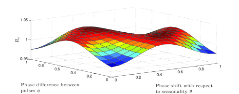
A natural question to ask is how does the relative timing of the pulse vaccinations in the two individual patches affect the global dynamics of the disease. By Theorems 3 and 4, the effective reproduction number Resubscript𝑅𝑒R_{e} provides a global threshold. Thus it suffices to determine how the phase difference between pulse vaccinations in the two patches affects the value of Resubscript𝑅𝑒R_{e}. In general, Resubscript𝑅𝑒R_{e} cannot be calculated explicitly. However, in the special case of no cross-infection or movement of infected individuals — i.e., f1=f2=0subscript𝑓1subscript𝑓20f_{1}=f_{2}=0 and k1=k2=0subscript𝑘1subscript𝑘20k_{1}=k_{2}=0Resubscript𝑅𝑒R_{e} can be formulated; furthermore, the effect of ϕitalic-ϕ\phi on Resubscript𝑅𝑒R_{e} can be quantified. In particular, we can prove that pulse synchronisation (ϕ=0italic-ϕ0\phi=0) minimizes (locally) the reproduction number Resubscript𝑅𝑒R_{e}. The details are contained in the following theorem.

Theorem 5.

Consider the two-patch model (19) with phase difference ϕitalic-ϕ\phi\in\mathbb{R} between pulse vaccinations and no cross-infection or movement of infected individuals; i.e., f1=f2=0subscript𝑓1subscript𝑓20f_{1}=f_{2}=0 and k1=k2=0subscript𝑘1subscript𝑘20k_{1}=k_{2}=0. Let S¯1ϕ(t)superscriptsubscript¯𝑆1italic-ϕ𝑡\overline{S}_{1}^{\phi}(t) and S¯2ϕ(t)superscriptsubscript¯𝑆2italic-ϕ𝑡\overline{S}_{2}^{\phi}(t) be the disease-free periodic solutions given by Proposition 2 parametrized by the phase difference ϕitalic-ϕ\phi. Then

Re(ϕ)=maxi=1,2{1(μi+γi)τ0τβi(t)S¯iϕ(t)𝑑t},subscript𝑅𝑒italic-ϕsubscript𝑖121subscript𝜇𝑖subscript𝛾𝑖𝜏superscriptsubscript0𝜏subscript𝛽𝑖𝑡superscriptsubscript¯𝑆𝑖italic-ϕ𝑡differential-d𝑡\displaystyle R_{e}(\phi)=\max_{i=1,2}\left\{\frac{1}{(\mu_{i}+\gamma_{i})\tau}\int_{0}^{\tau}\beta_{i}(t)\overline{S}_{i}^{\phi}(t)\,dt\right\}, (20)

where the reproduction number is a τ𝜏\tau-periodic function of ϕitalic-ϕ\phi on \mathbb{R}. Suppose further that the patches are identical and transmission rates are constant; i.e., b1=b2=b,μ1=μ2=μ,β1(t)=β2(t)=β,γ1=γ2=γ,m1=m2=mformulae-sequencesubscript𝑏1subscript𝑏2𝑏subscript𝜇1subscript𝜇2𝜇subscript𝛽1𝑡subscript𝛽2𝑡𝛽subscript𝛾1subscript𝛾2𝛾subscript𝑚1subscript𝑚2𝑚b_{1}=b_{2}=b,\mu_{1}=\mu_{2}=\mu,\beta_{1}(t)=\beta_{2}(t)=\beta,\gamma_{1}=\gamma_{2}=\gamma,m_{1}=m_{2}=m and ψ1=ψ2=ψsubscript𝜓1subscript𝜓2𝜓\psi_{1}=\psi_{2}=\psi. Then Re(ϕ)subscript𝑅𝑒italic-ϕR_{e}(\phi) has a local minimum at ϕ=0italic-ϕ0\phi=0 (in-phase pulses) and a critical point at ϕ=τ/2italic-ϕ𝜏2\phi=\tau/2 (out-of-phase pulses). More precisely, Re(ϕ)subscript𝑅𝑒italic-ϕR_{e}(\phi) is continuous on \mathbb{R}, smooth on {nτ:n}conditional-set𝑛𝜏𝑛\mathbb{R}\setminus\left\{n\tau:n\in\mathbb{Z}\right\} and

Re(0+)superscriptsubscript𝑅𝑒superscript0\displaystyle R_{e}^{\prime}(0^{+}) =R^0mψ2(eμτ1)22τ(eμτ(1ψ))2>0,Re(0)(=Re(τ))=Re(0+)<0,Re(τ2)=0,formulae-sequenceabsentsubscript^𝑅0𝑚superscript𝜓2superscriptsuperscript𝑒𝜇𝜏122𝜏superscriptsuperscript𝑒𝜇𝜏1𝜓20annotatedsuperscriptsubscript𝑅𝑒superscript0absentsuperscriptsubscript𝑅𝑒superscript𝜏superscriptsubscript𝑅𝑒superscript00superscriptsubscript𝑅𝑒𝜏20\displaystyle=\widehat{R}_{0}\frac{m\psi^{2}(e^{\mu\tau}-1)^{2}}{2\tau\left(e^{\mu\tau}-(1-\psi)\right)^{2}}>0,\qquad R_{e}^{\prime}(0^{-})\ \Big{(}=R_{e}^{\prime}(\tau^{-})\Big{)}\ =-R_{e}^{\prime}(0^{+})<0,\qquad R_{e}^{\prime}\left(\frac{\tau}{2}\right)=0,

where R^0=βbμ(μ+γ)subscript^𝑅0𝛽𝑏𝜇𝜇𝛾\widehat{R}_{0}=\frac{\beta b}{\mu(\mu+\gamma)} is the reproduction number of the (identical patch) system in the absence of pulse vaccination.

Proof.

Consider the two-patch model (19). Define the following linear system as in (11):

dwdt𝑑𝑤𝑑𝑡\displaystyle\frac{dw}{dt} =[V+Fϕ(t)λ]w,t,formulae-sequenceabsentdelimited-[]𝑉subscript𝐹italic-ϕ𝑡𝜆𝑤𝑡\displaystyle=\left[-V+\frac{F_{\phi}(t)}{\lambda}\right]w,\quad t\in\mathbb{R}, (21)

where

V=(μ1+γ1+k1k2k1μ2+γ2+k2),Fϕ(t)=(β1(t)S¯1ϕ(t)(1f1)β1(t)S¯1ϕ(t)f1β2(t)S¯2ϕ(t)f2β2(t)S¯2ϕ(t)(1f2)).formulae-sequence𝑉matrixsubscript𝜇1subscript𝛾1subscript𝑘1subscript𝑘2subscript𝑘1subscript𝜇2subscript𝛾2subscript𝑘2subscript𝐹italic-ϕ𝑡matrixsubscript𝛽1𝑡superscriptsubscript¯𝑆1italic-ϕ𝑡1subscript𝑓1subscript𝛽1𝑡superscriptsubscript¯𝑆1italic-ϕ𝑡subscript𝑓1subscript𝛽2𝑡superscriptsubscript¯𝑆2italic-ϕ𝑡subscript𝑓2subscript𝛽2𝑡superscriptsubscript¯𝑆2italic-ϕ𝑡1subscript𝑓2V=\begin{pmatrix}\mu_{1}+\gamma_{1}+k_{1}&-k_{2}\\ -k_{1}&\mu_{2}+\gamma_{2}+k_{2}\end{pmatrix},\qquad F_{\phi}(t)=\begin{pmatrix}\beta_{1}(t)\overline{S}_{1}^{\phi}(t)(1-f_{1})&\beta_{1}(t)\overline{S}_{1}^{\phi}(t)f_{1}\\ \beta_{2}(t)\overline{S}_{2}^{\phi}(t)f_{2}&\beta_{2}(t)\overline{S}_{2}^{\phi}(t)(1-f_{2})\end{pmatrix}.

Define the principle fundamental solution of (21) as Wϕ(t,λ)subscript𝑊italic-ϕ𝑡𝜆W_{\phi}(t,\lambda). Then the reproduction number as a function of ϕitalic-ϕ\phi, Re(ϕ)subscript𝑅𝑒italic-ϕR_{e}(\phi), is defined as the unique value of λ𝜆\lambda such that the dominant Floquet multiplier of (21) is one; i.e., ρ(Wϕ(τ,λ))=1𝜌subscript𝑊italic-ϕ𝜏𝜆1\rho(W_{\phi}(\tau,\lambda))=1. Clearly Re(ϕ)subscript𝑅𝑒italic-ϕR_{e}(\phi) is a τ𝜏\tau-periodic function. If k1=k2=f1=f2=0subscript𝑘1subscript𝑘2subscript𝑓1subscript𝑓20k_{1}=k_{2}=f_{1}=f_{2}=0, then the matrix Bϕ(t,λ)V+Fϕ(t)λsubscript𝐵italic-ϕ𝑡𝜆𝑉subscript𝐹italic-ϕ𝑡𝜆B_{\phi}(t,\lambda)\equiv-V+\frac{F_{\phi}(t)}{\lambda} is diagonal. Thus, as noted in [36] for diagonal systems, the eigenvalues of Wϕ(τ,λ)subscript𝑊italic-ϕ𝜏𝜆W_{\phi}(\tau,\lambda) are ri=(μi+γi)τ+1λ0τβi(t)S¯iϕ(t)𝑑tsubscript𝑟𝑖subscript𝜇𝑖subscript𝛾𝑖𝜏1𝜆superscriptsubscript0𝜏subscript𝛽𝑖𝑡superscriptsubscript¯𝑆𝑖italic-ϕ𝑡differential-d𝑡r_{i}=-(\mu_{i}+\gamma_{i})\tau+\frac{1}{\lambda}\int_{0}^{\tau}\beta_{i}(t)\overline{S}_{i}^{\phi}(t)\,dt, for i=1,2𝑖12i=1,2. It follows that

Re(ϕ)=maxi=1,2(1(μi+γi)τ0τβi(t)S¯iϕ(t)𝑑t).subscript𝑅𝑒italic-ϕsubscript𝑖121subscript𝜇𝑖subscript𝛾𝑖𝜏superscriptsubscript0𝜏subscript𝛽𝑖𝑡superscriptsubscript¯𝑆𝑖italic-ϕ𝑡differential-d𝑡R_{e}(\phi)=\max_{i=1,2}\Big{(}\frac{1}{(\mu_{i}+\gamma_{i})\tau}\int_{0}^{\tau}\beta_{i}(t)\overline{S}_{i}^{\phi}(t)\,dt\Big{)}.

In order to compute the derivative of Re(ϕ)subscript𝑅𝑒italic-ϕR_{e}(\phi), let ϕ>0italic-ϕ0\phi>0 and define R(ϕ)superscript𝑅italic-ϕR^{\prime}(\phi), and R(ϕ+)superscript𝑅superscriptitalic-ϕR^{\prime}(\phi^{+}) and Re(ϕ)superscriptsubscript𝑅𝑒superscriptitalic-ϕR_{e}^{\prime}(\phi^{-}) as the derivative and one-sided derivatives of Re(ϕ)subscript𝑅𝑒italic-ϕR_{e}(\phi) respectively. Consider the eigenvalue r(λ,ϕ)=ρ(Wϕ(τ,λ))𝑟𝜆italic-ϕ𝜌subscript𝑊italic-ϕ𝜏𝜆r(\lambda,\phi)=\rho(W_{\phi}(\tau,\lambda)). The characteristic equation is

r(λ,ϕ)2trWϕ(τ,λ)r(λ,ϕ)+detWϕ(τ,λ)=0.𝑟superscript𝜆italic-ϕ2trsubscript𝑊italic-ϕ𝜏𝜆𝑟𝜆italic-ϕsubscript𝑊italic-ϕ𝜏𝜆0r(\lambda,\phi)^{2}-{\rm tr}W_{\phi}(\tau,\lambda)r(\lambda,\phi)+\det W_{\phi}(\tau,\lambda)=0.

Then, since r(Re(ϕ),ϕ)=1𝑟subscript𝑅𝑒italic-ϕitalic-ϕ1r(R_{e}(\phi),\phi)=1 for all ϕitalic-ϕ\phi, we obtain:

detWϕ(τ,Re(ϕ))subscript𝑊italic-ϕ𝜏subscript𝑅𝑒italic-ϕ\displaystyle\det W_{\phi}(\tau,R_{e}(\phi)) =trWϕ(τ,Re(ϕ))1absenttrsubscript𝑊italic-ϕ𝜏subscript𝑅𝑒italic-ϕ1\displaystyle={\rm tr}W_{\phi}(\tau,R_{e}(\phi))-1
exp(0τtrBϕ(t,Re(ϕ))𝑑t)absentexpsuperscriptsubscript0𝜏trsubscript𝐵italic-ϕ𝑡subscript𝑅𝑒italic-ϕdifferential-d𝑡\displaystyle\Leftrightarrow{\rm exp}\left(\int_{0}^{\tau}{\rm tr}B_{\phi}(t,R_{e}(\phi))\,dt\right) =trWϕ(τ,Re(ϕ))1(by Liouville’s formula)absenttrsubscript𝑊italic-ϕ𝜏subscript𝑅𝑒italic-ϕ1(by Liouville’s formula)\displaystyle={\rm tr}W_{\phi}(\tau,R_{e}(\phi))-1\qquad\text{(by Liouville's formula)}
Thusϕexp(0τtrBϕ(t,Re(ϕ))𝑑t)Thusitalic-ϕexpsuperscriptsubscript0𝜏trsubscript𝐵italic-ϕ𝑡subscript𝑅𝑒italic-ϕdifferential-d𝑡\displaystyle\text{Thus}\ \ \frac{\partial}{\partial\phi}{\rm exp}\left(\int_{0}^{\tau}{\rm tr}B_{\phi}(t,R_{e}(\phi))\,dt\right) =ϕtrWϕ(τ,Re(ϕ)).absentitalic-ϕtrsubscript𝑊italic-ϕ𝜏subscript𝑅𝑒italic-ϕ\displaystyle=\frac{\partial}{\partial\phi}{\rm tr}W_{\phi}(\tau,R_{e}(\phi)).

Calculating the derivative with respect to ϕitalic-ϕ\phi, we obtain:

exp(0τtrBϕ(t,Re(ϕ))𝑑t)1Re(ϕ)[ϕ0τtrFϕ(t)𝑑tRe(ϕ)Re(ϕ)0τtrFϕ(t)𝑑t]=ϕtrWϕ(τ,Re(ϕ)).expsuperscriptsubscript0𝜏trsubscript𝐵italic-ϕ𝑡subscript𝑅𝑒italic-ϕdifferential-d𝑡1subscript𝑅𝑒italic-ϕdelimited-[]italic-ϕsuperscriptsubscript0𝜏trsubscript𝐹italic-ϕ𝑡differential-d𝑡superscriptsubscript𝑅𝑒italic-ϕsubscript𝑅𝑒italic-ϕsuperscriptsubscript0𝜏trsubscript𝐹italic-ϕ𝑡differential-d𝑡italic-ϕtrsubscript𝑊italic-ϕ𝜏subscript𝑅𝑒italic-ϕ\displaystyle{\rm exp}\left(\int_{0}^{\tau}{\rm tr}B_{\phi}(t,R_{e}(\phi))\,dt\right)\frac{1}{R_{e}(\phi)}\left[\frac{\partial}{\partial\phi}\int_{0}^{\tau}{\rm tr}F_{\phi}(t)\,dt-\frac{R_{e}^{\prime}(\phi)}{R_{e}(\phi)}\int_{0}^{\tau}{\rm tr}F_{\phi}(t)\,dt\right]=\frac{\partial}{\partial\phi}{\rm tr}W_{\phi}(\tau,R_{e}(\phi)). (22)

In the case that Bϕ(t,Re(ϕ))subscript𝐵italic-ϕ𝑡subscript𝑅𝑒italic-ϕB_{\phi}(t,R_{e}(\phi)) is diagonal — i.e., k1=k2=f1=f2=0subscript𝑘1subscript𝑘2subscript𝑓1subscript𝑓20k_{1}=k_{2}=f_{1}=f_{2}=0 — then Wϕ(τ,Re(ϕ))=exp(0τBϕ(t,Re(ϕ))𝑑t)subscript𝑊italic-ϕ𝜏subscript𝑅𝑒italic-ϕexpsuperscriptsubscript0𝜏subscript𝐵italic-ϕ𝑡subscript𝑅𝑒italic-ϕdifferential-d𝑡W_{\phi}(\tau,R_{e}(\phi))={\rm exp}\left(\int_{0}^{\tau}B_{\phi}(t,R_{e}(\phi))\,dt\right). Therefore

ϕtrWϕ(τ,Re(ϕ))italic-ϕtrsubscript𝑊italic-ϕ𝜏subscript𝑅𝑒italic-ϕ\displaystyle\frac{\partial}{\partial\phi}{\rm tr}W_{\phi}(\tau,R_{e}(\phi)) =i=12e(μi+γi)τRe(ϕ)[ϕ0τβi(t)S¯iϕ(t)𝑑tRe(ϕ)Re(ϕ)0τβi(t)S¯iϕ(t)𝑑t].absentsuperscriptsubscript𝑖12superscript𝑒subscript𝜇𝑖subscript𝛾𝑖𝜏subscript𝑅𝑒italic-ϕdelimited-[]italic-ϕsuperscriptsubscript0𝜏subscript𝛽𝑖𝑡superscriptsubscript¯𝑆𝑖italic-ϕ𝑡differential-d𝑡superscriptsubscript𝑅𝑒italic-ϕsubscript𝑅𝑒italic-ϕsuperscriptsubscript0𝜏subscript𝛽𝑖𝑡superscriptsubscript¯𝑆𝑖italic-ϕ𝑡differential-d𝑡\displaystyle=\sum_{i=1}^{2}{\frac{e^{-(\mu_{i}+\gamma_{i})\tau}}{R_{e}(\phi)}\left[\frac{\partial}{\partial\phi}\int_{0}^{\tau}\beta_{i}(t)\overline{S}_{i}^{\phi}(t)\,dt-\frac{R_{e}^{\prime}(\phi)}{R_{e}(\phi)}\int_{0}^{\tau}\beta_{i}(t)\overline{S}_{i}^{\phi}(t)\,dt\right].}

At this stage, we assume that μ1=μ2=μsubscript𝜇1subscript𝜇2𝜇\mu_{1}=\mu_{2}=\mu and γ1=γ2=γsubscript𝛾1subscript𝛾2𝛾\gamma_{1}=\gamma_{2}=\gamma. Inserting the above equation into (22), simplifying, and solving for Re(ϕ)superscriptsubscript𝑅𝑒italic-ϕR_{e}^{\prime}(\phi), we obtain:

Re(ϕ)superscriptsubscript𝑅𝑒italic-ϕ\displaystyle R_{e}^{\prime}(\phi) =Re(ϕ)ϕ[0τ(β1(t)S¯1ϕ(t)+β2(t)S¯2ϕ(t))𝑑t]0τ(β1(t)S¯1ϕ(t)+β2(t)S¯2ϕ(t))𝑑t.absentsubscript𝑅𝑒italic-ϕitalic-ϕdelimited-[]superscriptsubscript0𝜏subscript𝛽1𝑡superscriptsubscript¯𝑆1italic-ϕ𝑡subscript𝛽2𝑡superscriptsubscript¯𝑆2italic-ϕ𝑡differential-d𝑡superscriptsubscript0𝜏subscript𝛽1𝑡superscriptsubscript¯𝑆1italic-ϕ𝑡subscript𝛽2𝑡superscriptsubscript¯𝑆2italic-ϕ𝑡differential-d𝑡\displaystyle=R_{e}(\phi)\frac{\frac{\partial}{\partial\phi}\left[\int_{0}^{\tau}\left(\beta_{1}(t)\overline{S}_{1}^{\phi}(t)+\beta_{2}(t)\overline{S}_{2}^{\phi}(t)\right)\,dt\right]}{\int_{0}^{\tau}\left(\beta_{1}(t)\overline{S}_{1}^{\phi}(t)+\beta_{2}(t)\overline{S}_{2}^{\phi}(t)\right)\,dt}. (23)

The above formula shows that, under the prescribed assumptions, the relative change in Resubscript𝑅𝑒R_{e} with respect to the parameter ϕitalic-ϕ\phi is equal to the relative change (with respect to ϕitalic-ϕ\phi) in total force of infection summed over both patches and averaged over the period τ𝜏\tau. In the case that β1(t)=β2(t)=βsubscript𝛽1𝑡subscript𝛽2𝑡𝛽\beta_{1}(t)=\beta_{2}(t)=\beta is constant, β𝛽\beta cancels in formula (23) and we only need to consider the effect of ϕitalic-ϕ\phi on the total susceptible population among the patches averaged over the period.

Adding the differential equations of the disease-free τ𝜏\tau periodic solutions and integrating over the period τ𝜏\tau, we have

0=0τddt(S¯1ϕ(t)+S¯2ϕ(t))𝑑t0superscriptsubscript0𝜏𝑑𝑑𝑡superscriptsubscript¯𝑆1italic-ϕ𝑡superscriptsubscript¯𝑆2italic-ϕ𝑡differential-d𝑡\displaystyle 0=\int_{0}^{\tau}\frac{d}{dt}\left(\overline{S}_{1}^{\phi}(t)+\overline{S}_{2}^{\phi}(t)\right)\,dt =(b1+b2)τμ0τ(S¯1ϕ(t)+S¯2ϕ(t))𝑑t0τ(ψ1δ0S¯1ϕ(t)+ψ2δϕS¯2ϕ(t))𝑑t,absentsubscript𝑏1subscript𝑏2𝜏𝜇superscriptsubscript0𝜏superscriptsubscript¯𝑆1italic-ϕ𝑡superscriptsubscript¯𝑆2italic-ϕ𝑡differential-d𝑡superscriptsubscript0𝜏subscript𝜓1subscript𝛿0superscriptsubscript¯𝑆1italic-ϕ𝑡subscript𝜓2subscript𝛿italic-ϕsuperscriptsubscript¯𝑆2italic-ϕ𝑡differential-d𝑡\displaystyle=(b_{1}+b_{2})\tau-\mu\int_{0}^{\tau}\left(\overline{S}_{1}^{\phi}(t)+\overline{S}_{2}^{\phi}(t)\right)\,dt-\int_{0}^{\tau}\left(\psi_{1}\delta_{0}\overline{S}_{1}^{\phi}(t)+\psi_{2}\delta_{\phi}\overline{S}_{2}^{\phi}(t)\right)\,dt,

where δϕsubscript𝛿italic-ϕ\delta_{\phi} is the Dirac delta mass centred at ϕitalic-ϕ\phi. Thus

0τ(S¯1ϕ(t)+S¯2ϕ(t))𝑑tsuperscriptsubscript0𝜏superscriptsubscript¯𝑆1italic-ϕ𝑡superscriptsubscript¯𝑆2italic-ϕ𝑡differential-d𝑡\displaystyle\int_{0}^{\tau}\left(\overline{S}_{1}^{\phi}(t)+\overline{S}_{2}^{\phi}(t)\right)\,dt =1μ[(b1+b2)τ(ψ1S¯1ϕ(0)+ψ2S¯2ϕ(ϕ))].absent1𝜇delimited-[]subscript𝑏1subscript𝑏2𝜏subscript𝜓1superscriptsubscript¯𝑆1italic-ϕsuperscript0subscript𝜓2superscriptsubscript¯𝑆2italic-ϕsuperscriptitalic-ϕ\displaystyle=\frac{1}{\mu}\left[(b_{1}+b_{2})\tau-\left(\psi_{1}\overline{S}_{1}^{\phi}(0^{-})+\psi_{2}\overline{S}_{2}^{\phi}(\phi^{-})\right)\right]. (24)

Let

A=(μm1m2m1μm2).𝐴matrix𝜇subscript𝑚1subscript𝑚2subscript𝑚1𝜇subscript𝑚2A=\begin{pmatrix}-\mu-m_{1}&m_{2}\\ m_{1}&-\mu-m_{2}\end{pmatrix}.

As in the earlier formula (6), define the initial point of the disease-free periodic solution x¯=(S¯1ϕ(0),S¯2ϕ(0))T¯𝑥superscriptsuperscriptsubscript¯𝑆1italic-ϕsuperscript0superscriptsubscript¯𝑆2italic-ϕsuperscript0𝑇\overline{x}=\left(\overline{S}_{1}^{\phi}(0^{-}),\overline{S}_{2}^{\phi}(0^{-})\right)^{T}, along with the matrices D1=diag(1ψ1,1)subscript𝐷1diag1subscript𝜓11D_{1}={\rm diag}(1-\psi_{1},1), D2=diag(1,1ψ2)subscript𝐷2diag11subscript𝜓2D_{2}={\rm diag}(1,1-\psi_{2}), C2=e(τϕ)AD2subscript𝐶2superscript𝑒𝜏italic-ϕ𝐴subscript𝐷2C_{2}=e^{(\tau-\phi)A}D_{2}, C=C2eϕAD1𝐶subscript𝐶2superscript𝑒italic-ϕ𝐴subscript𝐷1C=C_{2}e^{\phi A}D_{1}. Also define x¯ϕ=(S¯1ϕ(ϕ),S¯2ϕ(ϕ))Tsubscript¯𝑥italic-ϕsuperscriptsuperscriptsubscript¯𝑆1italic-ϕsuperscriptitalic-ϕsuperscriptsubscript¯𝑆2italic-ϕsuperscriptitalic-ϕ𝑇\overline{x}_{\phi}=\left(\overline{S}_{1}^{\phi}(\phi^{-}),\overline{S}_{2}^{\phi}(\phi^{-})\right)^{T}. Then

x¯=(IC)1(C2(eϕAI)+e(τϕ)AI)A1b,x¯ϕ=eϕAD1x¯+(eϕAI)A1b.formulae-sequence¯𝑥superscript𝐼𝐶1subscript𝐶2superscript𝑒italic-ϕ𝐴𝐼superscript𝑒𝜏italic-ϕ𝐴𝐼superscript𝐴1𝑏subscript¯𝑥italic-ϕsuperscript𝑒italic-ϕ𝐴subscript𝐷1¯𝑥superscript𝑒italic-ϕ𝐴𝐼superscript𝐴1𝑏\overline{x}=(I-C)^{-1}\left(C_{2}(e^{\phi A}-I)+e^{(\tau-\phi)A}-I\right)A^{-1}b,\qquad\overline{x}_{\phi}=e^{\phi A}D_{1}\overline{x}+\left(e^{\phi A}-I\right)A^{-1}b.

All times are considered to be moduloτmodulo𝜏{\rm modulo}\ \tau. It can be inferred from these equations, along with (24) and (23), that Re(ϕ)superscriptsubscript𝑅𝑒italic-ϕR_{e}^{\prime}(\phi) is continuous on the set [0,τ)0𝜏[0,\tau) (where the interval is identified topologically as a circle glued together at the endpoints) and continuously differentiable on the set (0,τ)0𝜏(0,\tau). We further assume that m=m1=m2𝑚subscript𝑚1subscript𝑚2m=m_{1}=m_{2}, ψ=ψ1=ψ2𝜓subscript𝜓1subscript𝜓2\psi=\psi_{1}=\psi_{2}. Inserting the above formulas into (24), utilising (23), and evaluating /ϕitalic-ϕ\partial/\partial\phi at ϕ=0+italic-ϕsuperscript0\phi=0^{+}, ϕ=0italic-ϕsuperscript0\phi=0^{-} and ϕ=τ/2italic-ϕ𝜏2\phi=\tau/2, we find the following information:

Re(0+)superscriptsubscript𝑅𝑒superscript0\displaystyle R_{e}^{\prime}(0^{+}) =ψ2mb(eμτ1)2μ(1ψeμτ)2Re(ϕ)0τ(S¯10(t)+S¯20(t))𝑑t=R^0mψ2(eμτ1)22τ(eμτ(1ψ))2>0absentsuperscript𝜓2𝑚𝑏superscriptsuperscript𝑒𝜇𝜏12𝜇superscript1𝜓superscript𝑒𝜇𝜏2subscript𝑅𝑒italic-ϕsuperscriptsubscript0𝜏superscriptsubscript¯𝑆10𝑡superscriptsubscript¯𝑆20𝑡differential-d𝑡subscript^𝑅0𝑚superscript𝜓2superscriptsuperscript𝑒𝜇𝜏122𝜏superscriptsuperscript𝑒𝜇𝜏1𝜓20\displaystyle=\frac{\psi^{2}mb\left(e^{\mu\tau}-1\right)^{2}}{\mu\left(1-\psi-e^{\mu\tau}\right)^{2}}\cdot\frac{R_{e}(\phi)}{\int_{0}^{\tau}\left(\overline{S}_{1}^{0}(t)+\overline{S}_{2}^{0}(t)\right)\,dt}=\widehat{R}_{0}\frac{m\psi^{2}(e^{\mu\tau}-1)^{2}}{2\tau\left(e^{\mu\tau}-(1-\psi)\right)^{2}}>0 (25)
Re(0)superscriptsubscript𝑅𝑒superscript0\displaystyle R_{e}^{\prime}(0^{-}) =Re(τ)=ψ2mb(eμτ1)2μ(1ψeμτ)2Re(ϕ)0τ(S¯1ϕ(t)+S¯2ϕ(t))𝑑t=Re(0+)<0absentsuperscriptsubscript𝑅𝑒superscript𝜏superscript𝜓2𝑚𝑏superscriptsuperscript𝑒𝜇𝜏12𝜇superscript1𝜓superscript𝑒𝜇𝜏2subscript𝑅𝑒italic-ϕsuperscriptsubscript0𝜏superscriptsubscript¯𝑆1italic-ϕ𝑡superscriptsubscript¯𝑆2italic-ϕ𝑡differential-d𝑡superscriptsubscript𝑅𝑒superscript00\displaystyle=R_{e}^{\prime}(\tau^{-})=\frac{-\psi^{2}mb\left(e^{\mu\tau}-1\right)^{2}}{\mu\left(1-\psi-e^{\mu\tau}\right)^{2}}\cdot\frac{R_{e}(\phi)}{\int_{0}^{\tau}\left(\overline{S}_{1}^{\phi}(t)+\overline{S}_{2}^{\phi}(t)\right)\,dt}=-R_{e}^{\prime}(0^{+})<0 (26)
Re(τ2)superscriptsubscript𝑅𝑒𝜏2\displaystyle R_{e}^{\prime}\left(\frac{\tau}{2}\right) =0.absent0\displaystyle=0. (27)

Remarks. 1. The explicit formula for Re(0+)superscriptsubscript𝑅𝑒superscript0R_{e}^{\prime}(0^{+}) can tell us which parameters affect the sensitivity of Resubscript𝑅𝑒R_{e} to ϕitalic-ϕ\phi. In particular, Re(0+)superscriptsubscript𝑅𝑒superscript0R_{e}^{\prime}(0^{+}) is increasing with respect to the migration rate m𝑚m, the “natural” effective reproduction number R^0subscript^𝑅0\widehat{R}_{0}, the death rate μ𝜇\mu and the pulse vaccination proportion ψ𝜓\psi. Thus an increase in any of these parameters results in larger increases in Resubscript𝑅𝑒R_{e} when the pulse vaccinations in the two patches are perturbed away from synchrony.
2. While it would be nice to obtain more general results, the mathematical complexity of the system is difficult to overcome. We suspect that ϕ=0italic-ϕ0\phi=0 is the global minimum, but the formulas for Re(ϕ)subscript𝑅𝑒italic-ϕR_{e}(\phi) and Re(ϕ)superscriptsubscript𝑅𝑒italic-ϕR_{e}^{\prime}(\phi) are difficult to analyze at other values of ϕitalic-ϕ\phi. We note that simulations show that, for small enough values of migration rate m𝑚m, ϕ=τ/2italic-ϕ𝜏2\phi=\tau/2 corresponds to a global maximum of Re(ϕ)subscript𝑅𝑒italic-ϕR_{e}(\phi). However, for large migration rates m𝑚m, ϕ=τ/2italic-ϕ𝜏2\phi=\tau/2 may not correspond to a maximum, and simulations show there can be a value 0<ϕ<τ/20superscriptitalic-ϕ𝜏20<\phi^{*}<\tau/2 such that ϕ=ϕitalic-ϕsuperscriptitalic-ϕ\phi=\phi^{*} and ϕ=τϕitalic-ϕ𝜏superscriptitalic-ϕ\phi=\tau-\phi^{*}, which are both global maxima of Re(ϕ)subscript𝑅𝑒italic-ϕR_{e}(\phi). See Figure 2.
3. It would be nice to remove the assumption of no cross-infection or migration of infected individuals. However, the linear periodic system cannot generally be solved in this case, since Bϕ(t,λ)V+Fϕ(t)λsubscript𝐵italic-ϕ𝑡𝜆𝑉subscript𝐹italic-ϕ𝑡𝜆B_{\phi}(t,\lambda)\equiv-V+\frac{F_{\phi}(t)}{\lambda} is not diagonal. The system can be explicitly solved in this case when ϕ=0italic-ϕ0\phi=0 and the patches are identical (since B0(t,λ)subscript𝐵0𝑡𝜆B_{0}(t,\lambda) commutes with its integral in this case), but a perturbation in ϕitalic-ϕ\phi is very difficult to analyze, and we leave this as future work.
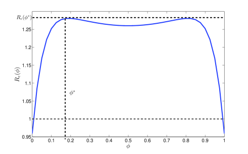
Refer to caption
Figure 2: Example of large migration rates producing two global maxima of Re(ϕ)subscript𝑅𝑒italic-ϕR_{e}(\phi). Parameters used were m=10𝑚10m=10, R^0=20subscript^𝑅020\widehat{R}_{0}=20, μ=b=1/50𝜇𝑏150\mu=b=1/50, γ=365/16𝛾36516\gamma=365/16, and ψ=0.8𝜓0.8\psi=0.8.

In the next subsection, we provide simulations that illustrate the theorem and show that the implications hold in the case of cross-infection and migration of infected individuals. In addition, the pulse synchronisation result is explained in the context of mass-vaccination campaigns against polio and measles.

6.2 The SIR model with identical patches and no seasonality

For the simulations in this subsection, we choose parameters in line with poliomyelitis epidemiology. To isolate the effects of varying phase difference ϕitalic-ϕ\phi between the pulses, we set τ𝜏\tau to 1 year and suppose that the patches are “identical”: b1=b2=b,μ1=μ2=μ,β1(t)=β2(t)=β(t),γ1=γ2=γ,f1=f2=f,m1=m2=m,k1=k2=mformulae-sequencesubscript𝑏1subscript𝑏2𝑏subscript𝜇1subscript𝜇2𝜇subscript𝛽1𝑡subscript𝛽2𝑡𝛽𝑡subscript𝛾1subscript𝛾2𝛾subscript𝑓1subscript𝑓2𝑓subscript𝑚1subscript𝑚2𝑚subscript𝑘1subscript𝑘2𝑚b_{1}=b_{2}=b,\mu_{1}=\mu_{2}=\mu,\beta_{1}(t)=\beta_{2}(t)=\beta(t),\gamma_{1}=\gamma_{2}=\gamma,f_{1}=f_{2}=f,m_{1}=m_{2}=m,k_{1}=k_{2}=m and ψ1=ψ2=ψsubscript𝜓1subscript𝜓2𝜓\psi_{1}=\psi_{2}=\psi. Then, with no seasonality (i.e., β(t)=β𝛽𝑡𝛽\beta(t)=\beta constant),

R^0βbμ(μ+γ)subscript^𝑅0𝛽𝑏𝜇𝜇𝛾\displaystyle\widehat{R}_{0}\equiv\frac{\beta b}{\mu(\mu+\gamma)} (17)

is the basic reproduction number of the autonomous (no pulse vaccination) version of model (19) [23]. We remark that, in this case of identical patches, the “global” reproduction number of the autonomous model, R^0subscript^𝑅0\widehat{R}_{0}, is equal to the “patch” reproduction number. We also note that the above formula holds for the case k1=k2msubscript𝑘1subscript𝑘2𝑚k_{1}=k_{2}\neq m, but we assume that the migration rates for susceptibles and infected individuals are equal. This assumption may be reasonable for polio, since at least 95% of cases are asymptomatic [38].

The reproduction number for polio in an immunologically naïve population in low-income areas has been estimated in the range 6–14, although it has been speculated to be as high as 20 for some densely populated regions [17]. The mean infectious period for poliovirus is approximately 16 days [17]. The average lifespan of individuals in the population is assumed to be 50 years. Note that we will also vary the lifespan, in order to see its effect on Resubscript𝑅𝑒R_{e}. The total population size can be normalised to be 1 by letting b=μ𝑏𝜇b=\mu. Note that this can be done without loss of generality by dividing the equations in (19) by b/μ𝑏𝜇b/\mu, which rescales the variables as fractions of carrying capacity (in the absence of migration) b/μ𝑏𝜇b/\mu, and rescales the parameters b𝑏b and β𝛽\beta. Explicitly, the following parameters will be used in the following subsection: b=μ=1/50𝑏𝜇150b=\mu=1/50, γ=365/16𝛾36516\gamma=365/16, β=319.655𝛽319.655\beta=319.655. These parameters give a value of R^0=14subscript^𝑅014\widehat{R}_{0}=14, close to the upper bound of reproductive potential for poliovirus. The pulse vaccination proportions, ψ𝜓\psi, are taken to be ψ=0.231𝜓0.231\psi=0.231, in order to bring the reproduction number close to the threshold value of 111. This proportion may seem small, but it should be mentioned that vaccination campaigns only target children; therefore, 23.1%percent23.123.1\% represents a substantial percentage of children to vaccinate. The coupling parameter values depend on the specific regions of consideration. In the simulations below, the coupling parameters m𝑚m and f𝑓f will be varied and, in some instances, will be chosen relatively large to illustrate the effect of phase difference on Resubscript𝑅𝑒R_{e}. Also, a seasonal transmission rate will be introduced in Section 6.3. The aforementioned parameter values are given in Table 1, along with units and descriptions.

Table 1: Parameter values, units and description for case of identical patches
Parameter Value Units Meaning
b𝑏b 1/50 individuals×year1individualssuperscriptyear1{\rm individuals}\times{\rm year}^{-1} birth rate
μ𝜇\mu 1/50 year1superscriptyear1{\rm year}^{-1} death rate
β𝛽\beta 319.655 (individuals×year)1superscriptindividualsyear1\left({\rm individuals}\times{\rm year}\right)^{-1} transmission rate
γ𝛾\gamma (1/(16/365)) year1superscriptyear1{\rm year}^{-1} recovery rate
m,k𝑚𝑘m,k varied; 0m,k2formulae-sequence0𝑚𝑘20\leq m,k\leq 2 year1superscriptyear1{\rm year}^{-1} migration rate of susceptible and infected
f𝑓f varied; 0f1/20𝑓120\leq f\leq 1/2 fraction of cross transmission
ψ𝜓\psi 0.231 pulse vaccination proportion
τ𝜏\tau 1 years period
ϕitalic-ϕ\phi varied; 0ϕ10italic-ϕ10\leq\phi\leq 1 yearsyears{\rm years} phase difference between pulses
R^0subscript^𝑅0\widehat{R}_{0} 14 reproduction number for naïve population

First, consider the case where linear migration is included without seasonality or mass-action coupling of the patches; i.e., m>0𝑚0m>0, f=0𝑓0f=0 and β(t)=β=constant𝛽𝑡𝛽constant\beta(t)=\beta=\text{constant}. Numerical calculations of Resubscript𝑅𝑒R_{e} as the phase difference between the pulses varies are presented in Figure 3. Notice that Resubscript𝑅𝑒R_{e} is minimised when the pulses are in phase; i.e., when the patches synchronise their vaccination campaigns. Also, as the migration rate m𝑚m increases, Resubscript𝑅𝑒R_{e} becomes increasingly sensitive to the phase difference, ϕitalic-ϕ\phi. These observations are consistent with Theorem 5. Also, there is an intuitive explanation for this result. When regions coupled by migration employ pulse vaccination, we can think of how to best time the vaccination pulses in order to immunise as many migrants as possible. If the pulses are de-synchronised, then it is possible — even with 100% coverage in each patch — that a migrant (who is born at some time t0subscript𝑡0t_{0} and does not die during the period [t0,t0+τ]subscript𝑡0subscript𝑡0𝜏[t_{0},t_{0}+\tau]) can remain unvaccinated by being in Patch 2 when Patch 1 employs pulse vaccination and in Patch 1 when Patch 2 conducts their pulse vaccination. There is evidence that this effect has led to measles epidemics in the coupled regions of Burkina Faso and Côte d’Ivoire in Africa [41]. Synchronising the pulses can most effectively reach the migrant population. Indeed, when the average total susceptible population over the year is plotted with respect to ϕitalic-ϕ\phi, the graph has the same shape as Figure 3. In other words, synchronising the pulses will produce the highest time-averaged coverage for a fixed proportion, ψ𝜓\psi, of susceptibles that can be vaccinated in each pulse. This is of course expected from Theorem 5, where we prove these statements about synchronisation (locally and in a more restricted setting).
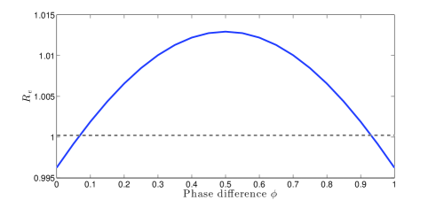
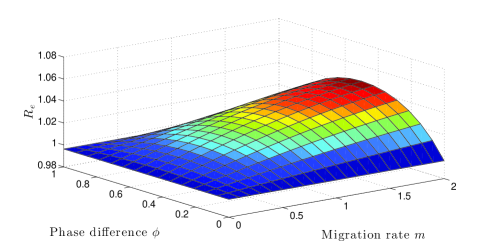
Refer to caption
Refer to caption
Figure 3: The effects of phase difference when the transmission rate is constant and there is only migration. (a) Resubscript𝑅𝑒R_{e} vs phase difference ϕitalic-ϕ\phi, for the case m=0.5𝑚0.5m=0.5. (b) Resubscript𝑅𝑒R_{e} vs phase difference ϕitalic-ϕ\phi and migration rate m𝑚m.

Next, suppose that the patches are only coupled through mass-action cross transmission without seasonality; i.e., 0f1/20𝑓120\leq f\leq 1/2, m=0𝑚0m=0 and β(t)=β𝛽𝑡𝛽\beta(t)=\beta. Figure 4 displays numerical calculations of Resubscript𝑅𝑒R_{e} versus the phase difference ϕitalic-ϕ\phi for this case. Again, Resubscript𝑅𝑒R_{e} is always minimised when the pulses are synchronised; i.e., ϕ=0italic-ϕ0\phi=0. However, this case is more subtle than the previous one. When the average total susceptible population over the year is taken as a function of the phase difference ϕitalic-ϕ\phi, it is not hard to see that this will be constant as ϕitalic-ϕ\phi varies between 00 and 111. Thus the optimality of pulse synchronisation cannot be explained like the previous case where the (averaged) susceptible population was minimised when ϕ=0italic-ϕ0\phi=0, and Theorem 5 cannot be applied. Also, observe that the phase difference becomes a non-factor as f1/2𝑓12f\rightarrow 1/2 in Figure 4. In this case, the contribution of cross transmission becomes equal to within-patch transmission when f1/2𝑓12f\rightarrow 1/2, causing the infected in a patch to have equal magnitude of correlation with either pulse. This is likely the reason that the phase difference does not affect Resubscript𝑅𝑒R_{e} when f=1/2𝑓12f=1/2.

Refer to caption
Refer to caption
Figure 4: The case when identical patches are coupled through mass-action cross transmission without seasonality. (a) Resubscript𝑅𝑒R_{e} vs phase difference ϕitalic-ϕ\phi for the coupling factor f=0.1𝑓0.1f=0.1. (b) Resubscript𝑅𝑒R_{e} vs phase difference ϕitalic-ϕ\phi and coupling factor f𝑓f.

Theorem 5 implies that Re(ϕ)subscript𝑅𝑒italic-ϕR_{e}(\phi), the reproduction number Resubscript𝑅𝑒R_{e} as a function of phase difference ϕitalic-ϕ\phi, may be most sensitive to ϕitalic-ϕ\phi when m𝑚m, R^0subscript^𝑅0\widehat{R}_{0}, ψ𝜓\psi and μ𝜇\mu are large; this is confirmed in simulations. From Figures 3 and 4, it is seen that the migration rate m𝑚m and coupling factor f𝑓f strongly affect the amplitude of Re(ϕ)subscript𝑅𝑒italic-ϕR_{e}(\phi). If the migration rate m𝑚m is large or if f𝑓f is close to a certain value (around 0.1 in Figure 4), pulse synchronisation becomes increasingly important, since Resubscript𝑅𝑒R_{e} can vary largely with ϕitalic-ϕ\phi. In Figure 5, observe that, as μ𝜇\mu and ψ𝜓\psi increases, while keeping b=μ𝑏𝜇b=\mu and fixing the other parameters, the amplitude of Re(ϕ)subscript𝑅𝑒italic-ϕR_{e}(\phi) increases. In Figure 5, we plot the pulse vaccination proportion ψ𝜓\psi required for Re=1subscript𝑅𝑒1R_{e}=1 as a function of ϕitalic-ϕ\phi for three different wild (before immunisation) reproduction numbers, R^0subscript^𝑅0\widehat{R}_{0}. As R^0subscript^𝑅0\widehat{R}_{0} increases, more vaccination is required to bring Resubscript𝑅𝑒R_{e} to unity and the “phase effect” increases. For the cases where the amplitude of Re(ϕ)subscript𝑅𝑒italic-ϕR_{e}(\phi) is relatively large, it is vital to synchronise the pulses since the parameter ϕitalic-ϕ\phi can be the difference between extinction and persistence of the pathogen. In Figure 6, there are simulations of the system (19) in the case of in-phase pulses (ϕ=0italic-ϕ0\phi=0), resulting in eradication, and out-of-phase pulses (ϕ=0.5italic-ϕ0.5\phi=0.5), resulting in disease persistence.
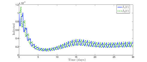
Refer to caption
Refer to caption
Figure 5: The effect of μ𝜇\mu, ψ𝜓\psi and R^0subscript^𝑅0\widehat{R}_{0} on Re(ϕ)subscript𝑅𝑒italic-ϕR_{e}(\phi). (a) Re(ϕ)subscript𝑅𝑒italic-ϕR_{e}(\phi) for three different values of μ𝜇\mu and ψ𝜓\psi with m=1𝑚1m=1, f=1𝑓1f=1 and all other parameters as in Table 1. (b) The pulse vaccination proportion ψ𝜓\psi required for Re=1subscript𝑅𝑒1R_{e}=1 as the phase difference ϕitalic-ϕ\phi varies for three different values of R^0subscript^𝑅0\widehat{R}_{0} with m=1𝑚1m=1, f=1𝑓1f=1 and all other parameters as in Table 1.
Refer to caption
Refer to caption
Figure 6: Simulations showing how the timing between the pulse vaccination can determine whether the disease persists. The coupling parameters are taken to be m=1𝑚1m=1 and f=0.1𝑓0.1f=0.1. (a) Simulation of the infected in Patches 1 and 2 when the vaccination pulses are synchronised; i.e., Ii(t)subscript𝐼𝑖𝑡I_{i}(t) when ϕ=0italic-ϕ0\phi=0. (b) Simulation of the infected in Patches 1 and 2 when the pulses are completely desynchronised; i.e., Ii(t)subscript𝐼𝑖𝑡I_{i}(t) when ϕ=0.5italic-ϕ0.5\phi=0.5. Identical patches are considered.

6.3 The SIR model with identical patches and seasonality

Now consider identical patches with seasonality, where β(t)=β(1+asin(2π(tθ)))𝛽𝑡𝛽1𝑎2𝜋𝑡𝜃\beta(t)=\beta(1+a\sin(2\pi(t-\theta))). Here θ𝜃\theta is a seasonal phase-shift parameter, which allows us to vary the timing of the pulses throughout the year. In the example simulated in Figure 7, it is optimal to synchronise the pulse vaccinations and to execute just before the high-transmission season. This finding agrees with results obtained for single patch SIR models [29]. The importance of synchronising the pulses increases with migration rate m𝑚m, while the sensitivity to timing the pulses with respect to seasonality increases with the seasonal forcing amplitude a𝑎a. Also, the sensitivity to timing pulses with respect to each other and seasonality both increase with ψ𝜓\psi, μ𝜇\mu, and R^0subscript^𝑅0\widehat{R}_{0}.

Refer to caption
Figure 7: Resubscript𝑅𝑒R_{e} vs phase difference between pulses for the system with seasonality. The seasonal transmission is of the form β(t)=β(1+asin(2π(tθ)))𝛽𝑡𝛽1𝑎2𝜋𝑡𝜃\beta(t)=\beta(1+a\sin(2\pi(t-\theta))) where θ𝜃\theta is the seasonal phase shift. Here a=0.5𝑎0.5a=0.5, the migration rate is m=0.5𝑚0.5m=0.5, there is no cross-transmission (f=0𝑓0f=0), and the other parameters are as in Table 1. In this case, the results show that it is best to synchronise pulse vaccinations and to execute them during the season before the high-transmission season.

If the seasonal transmission coefficients for the two patches are not in phase, then optimal timing of pulses with respect to seasonality can be in conflict with synchronising the pulses. This creates a trade-off between synchronising the pulses and optimally timing the pulse in each patch according to the transmission season. In the pulse vaccination operation against polio, Operation MECACAR, public health officials had to consider this trade-off [10]. In this case, they decided that pulse synchronisation was most important. Theoretically, the optimal timing of pulse vaccinations should depend on the specific parameters, especially the relative size of migration rate to seasonal forcing amplitude. To illustrate this phenomenon, we consider transmission rates β1(t)=β(1+asin(2π(tθ)))subscript𝛽1𝑡𝛽1𝑎2𝜋𝑡𝜃\beta_{1}(t)=\beta(1+a\sin(2\pi(t-\theta))) and β2(t)=β(1+asin(2π(tθσ)))subscript𝛽2𝑡𝛽1𝑎2𝜋𝑡𝜃𝜎\beta_{2}(t)=\beta(1+a\sin(2\pi(t-\theta-\sigma))) for Patch 1 and Patch 2, respectively. Here σ𝜎\sigma is the phase difference between the seasonal transmission rates of Patch 1 and Patch 2. In Figure 8, Resubscript𝑅𝑒R_{e} is calculated for the case where the seasonal transmission rates are out of phase; i.e., σ=0.5𝜎0.5\sigma=0.5. In Figure 8, the migration rate m𝑚m is set to 0.50.50.5 and the mass-action coupling f𝑓f is 00. For this case, the seasonal transmission has a larger effect than the migration, and it is best to desynchronise the pulses so that each pulse occurs in the season before the higher transmission season. In Figure 8, the migration rate is assumed to be larger (m=2𝑚2m=2); in this scenario, it is best to synchronise the pulses.
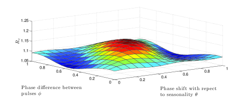
Refer to caption
Refer to caption
Figure 8: Resubscript𝑅𝑒R_{e} vs phase difference between pulses for the system with out-of-phase seasonal transmission rates. The seasonal transmission rates are of the form β1(t)=β(1+0.5sin(2π(tθ)))subscript𝛽1𝑡𝛽10.52𝜋𝑡𝜃\beta_{1}(t)=\beta(1+0.5\sin(2\pi(t-\theta))) and β2(t)=β(1+0.5sin(2π(tθ0.5)))subscript𝛽2𝑡𝛽10.52𝜋𝑡𝜃0.5\beta_{2}(t)=\beta(1+0.5\sin(2\pi(t-\theta-0.5))). In (a), the migration rate, m𝑚m, is set to 0.50.50.5. For this case, it is best to desynchronise pulses. In (b), the migration rate is set to 222, and it is best to synchronise the pulses. In both figures, there is no mass-action coupling (f=0)𝑓0(f=0) and the other parameters are specified in the text.
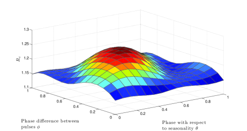
6.4 Comparison of vaccination strategies and effect of different movement scenarios on optimal vaccine distribution

An interesting and possibly applicable exercise is to compare a constant-vaccination strategy with the pulse-vaccination strategy. From a theoretical standpoint, it is important to reconcile results obtained for pulse vaccination with the findings for a smooth, constant vaccination rate. On the practical side, disease-control authorities may like to know the optimal vaccination strategy based on a simple cost measure. The basic measure that will be used to quantify the cost of a vaccination strategy is vaccinations per period τ𝜏\tau calculated at the disease-free periodic solution. From an economic perspective, this cost measure has the appeal of simplicity. To understand why this definition can also be the dynamically sound way of measuring cost, it is instructive to consider the case of isolated patches or, without loss of generality, a single patch under a general periodic vaccination strategy. Specifically, consider the following system:

dSdt𝑑𝑆𝑑𝑡\displaystyle\frac{dS}{dt} =bμSβ(t)SIζ(t)Sabsent𝑏𝜇𝑆𝛽𝑡𝑆𝐼𝜁𝑡𝑆\displaystyle=b-\mu S-\beta(t)SI-\zeta(t)S
dIdt𝑑𝐼𝑑𝑡\displaystyle\frac{dI}{dt} =β(t)SI(μ+γ)I,absent𝛽𝑡𝑆𝐼𝜇𝛾𝐼\displaystyle=\beta(t)SI-(\mu+\gamma)I,

where the ζ(t)𝜁𝑡\zeta(t) is a τ𝜏\tau-periodic vaccination rate and the transmission rate, β(t)𝛽𝑡\beta(t), is τ𝜏\tau-periodic. In the case of constant vaccination, ζ(t)σ𝜁𝑡𝜎\zeta(t)\equiv\sigma, where σ+𝜎subscript\sigma\in\mathbb{R}_{+}. For pulse vaccination, ζ(t)=nψδnτ𝜁𝑡subscript𝑛𝜓subscript𝛿𝑛𝜏\zeta(t)=\sum_{n\in\mathbb{N}}\psi\delta_{n\tau}, where δtsubscript𝛿𝑡\delta_{t} is the Dirac delta mass centred at t𝑡t and 0ψ10𝜓10\leq\psi\leq 1. In [29], the authors rigorously define the appropriate space of periodic vaccination rates to include the Dirac delta mass and guarantee existence of a unique disease-free susceptible periodic solution, S¯ζ(t)subscript¯𝑆𝜁𝑡\overline{S}_{\zeta}(t), for any periodic vaccination rate ζ(t)𝜁𝑡\zeta(t) in this setting. The cost of vaccination (vaccinations per period calculated at S¯ζ(t)subscript¯𝑆𝜁𝑡\overline{S}_{\zeta}(t)) is

Cζ0τζ(t)S¯ζ(t)𝑑t.subscript𝐶𝜁superscriptsubscript0𝜏𝜁𝑡subscript¯𝑆𝜁𝑡differential-d𝑡\displaystyle C_{\zeta}\equiv\int_{0}^{\tau}\zeta(t)\overline{S}_{\zeta}(t)\,dt.

Using the next-generation characterisation (11), the effective reproduction number, Resubscript𝑅𝑒R_{e}, can be explicitly found as

Re=1μ+γ1τ0τβ(t)S¯ζ(t)𝑑t.subscript𝑅𝑒1𝜇𝛾1𝜏superscriptsubscript0𝜏𝛽𝑡subscript¯𝑆𝜁𝑡differential-d𝑡\displaystyle R_{e}=\frac{1}{\mu+\gamma}\frac{1}{\tau}\int_{0}^{\tau}\beta(t)\overline{S}_{\zeta}(t)\,dt.

Onyango and Müller studied optimal vaccination strategies in this model in terms of minimising Resubscript𝑅𝑒R_{e} [29]. Here we give a simple representation of Resubscript𝑅𝑒R_{e} that can yield insight into comparing vaccination strategies, but do not provide the rigorous construction of the optimal strategy done by Onyango and Müller [29]. Specifically, we rewrite Resubscript𝑅𝑒R_{e} for a general periodic vaccination strategy ζ(t)𝜁𝑡\zeta(t) in a form that compares it to the constant-vaccination strategy of equal cost. First, as noted in [29], by integrating the S˙˙𝑆\dot{S} equation over one period, the following can be obtained:

Cζ=τbμ0τS¯ζ(t)𝑑t.subscript𝐶𝜁𝜏𝑏𝜇superscriptsubscript0𝜏subscript¯𝑆𝜁𝑡differential-d𝑡\displaystyle C_{\zeta}=\tau b-\mu\int_{0}^{\tau}\overline{S}_{\zeta}(t)\,dt.

Define the average transmission rate as β=1τ0τβ(t)𝑑tdelimited-⟨⟩𝛽1𝜏superscriptsubscript0𝜏𝛽𝑡differential-d𝑡\langle\beta\rangle=\frac{1}{\tau}\int_{0}^{\tau}\beta(t)\,dt. For constant vaccination, ζ1(t)σsubscript𝜁1𝑡𝜎\zeta_{1}(t)\equiv\sigma, so we find that Cζ1=σbτμ+σsubscript𝐶subscript𝜁1𝜎𝑏𝜏𝜇𝜎C_{\zeta_{1}}=\frac{\sigma b\tau}{\mu+\sigma} and the effective reproduction number is Rec=βb(μ+σ)(μ+γ)superscriptsubscript𝑅𝑒𝑐delimited-⟨⟩𝛽𝑏𝜇𝜎𝜇𝛾R_{e}^{c}=\frac{\langle\beta\rangle b}{(\mu+\sigma)(\mu+\gamma)}. For the periodic vaccination rate ζ(t)𝜁𝑡\zeta(t), we rewrite the effective reproduction number Resubscript𝑅𝑒R_{e} by comparing it to a constant-vaccination strategy of equal cost:

βσbτμ+σdelimited-⟨⟩𝛽𝜎𝑏𝜏𝜇𝜎\displaystyle\langle\beta\rangle\frac{\sigma b\tau}{\mu+\sigma} =βCζ1=βCζ=βτbβμ0τS¯ζ(t)𝑑tabsentdelimited-⟨⟩𝛽subscript𝐶subscript𝜁1delimited-⟨⟩𝛽subscript𝐶𝜁delimited-⟨⟩𝛽𝜏𝑏delimited-⟨⟩𝛽𝜇superscriptsubscript0𝜏subscript¯𝑆𝜁𝑡differential-d𝑡\displaystyle=\langle\beta\rangle C_{\zeta_{1}}=\langle\beta\rangle C_{\zeta}=\langle\beta\rangle\tau b-\langle\beta\rangle\mu\int_{0}^{\tau}\overline{S}_{\zeta}(t)\,dt
βσbτμ+σdelimited-⟨⟩𝛽𝜎𝑏𝜏𝜇𝜎\displaystyle\langle\beta\rangle\frac{\sigma b\tau}{\mu+\sigma} =βτbμ0τβ(t)S¯ζ(t)𝑑t+μ0τS¯(t)(β(t)β)𝑑tabsentdelimited-⟨⟩𝛽𝜏𝑏𝜇superscriptsubscript0𝜏𝛽𝑡subscript¯𝑆𝜁𝑡differential-d𝑡𝜇superscriptsubscript0𝜏¯𝑆𝑡𝛽𝑡delimited-⟨⟩𝛽differential-d𝑡\displaystyle=\langle\beta\rangle\tau b-\mu\int_{0}^{\tau}\beta(t)\overline{S}_{\zeta}(t)\,dt+\mu\int_{0}^{\tau}\overline{S}(t)(\beta(t)-\langle\beta\rangle)\,dt
βσbτμ+σdelimited-⟨⟩𝛽𝜎𝑏𝜏𝜇𝜎\displaystyle\langle\beta\rangle\frac{\sigma b\tau}{\mu+\sigma} =βτbμ(μ+γ)τRe+μ0τS¯ζ(t)(β(t)β)𝑑tabsentdelimited-⟨⟩𝛽𝜏𝑏𝜇𝜇𝛾𝜏subscript𝑅𝑒𝜇superscriptsubscript0𝜏subscript¯𝑆𝜁𝑡𝛽𝑡delimited-⟨⟩𝛽differential-d𝑡\displaystyle=\langle\beta\rangle\tau b-\mu(\mu+\gamma)\tau R_{e}+\mu\int_{0}^{\tau}\overline{S}_{\zeta}(t)(\beta(t)-\langle\beta\rangle)\,dt
Reabsentsubscript𝑅𝑒\displaystyle\Leftrightarrow R_{e} =Rec+1(μ+γ)τ0τS¯ζ(t)(β(t)β)𝑑t.absentsuperscriptsubscript𝑅𝑒𝑐1𝜇𝛾𝜏superscriptsubscript0𝜏subscript¯𝑆𝜁𝑡𝛽𝑡delimited-⟨⟩𝛽differential-d𝑡\displaystyle=R_{e}^{c}+\frac{1}{(\mu+\gamma)\tau}\int_{0}^{\tau}\overline{S}_{\zeta}(t)(\beta(t)-\langle\beta\rangle)\,dt.

If we normalise S¯ζ(t)subscript¯𝑆𝜁𝑡\overline{S}_{\zeta}(t) by letting s¯ζ(t)=μbS¯ζ(t)subscript¯𝑠𝜁𝑡𝜇𝑏subscript¯𝑆𝜁𝑡\bar{s}_{\zeta}(t)=\frac{\mu}{b}\overline{S}_{\zeta}(t) and denote R^0=βbμ(μ+γ)subscript^𝑅0delimited-⟨⟩𝛽𝑏𝜇𝜇𝛾\widehat{R}_{0}=\frac{\langle\beta\rangle b}{\mu(\mu+\gamma)} (the reproduction number in the absence of vaccination), then the following is obtained:

Re=RecR^01τ0τs¯ζ(t)(1β(t)β)𝑑t.subscript𝑅𝑒superscriptsubscript𝑅𝑒𝑐subscript^𝑅01𝜏superscriptsubscript0𝜏subscript¯𝑠𝜁𝑡1𝛽𝑡delimited-⟨⟩𝛽differential-d𝑡\displaystyle R_{e}=R_{e}^{c}-\widehat{R}_{0}\frac{1}{\tau}\int_{0}^{\tau}\overline{s}_{\zeta}(t)\left(1-\frac{\beta(t)}{\langle\beta\rangle}\right)\,dt.

Clearly, if β(t)𝛽𝑡\beta(t) is constant — i.e., β(t)=β𝛽𝑡delimited-⟨⟩𝛽\beta(t)=\langle\beta\rangle — then all vaccination strategies are equivalent, in particular pulse- and constant-vaccination strategies, and Re=Rcsubscript𝑅𝑒subscript𝑅𝑐R_{e}=R_{c}. This observation provides justification as to why Cζsubscript𝐶𝜁C_{\zeta} is an appropriate cost measure from an epidemiological point of view. When β(t)𝛽𝑡\beta(t) is not constant, then a different result is obtained. Define α(t)=1β(t)β𝛼𝑡1𝛽𝑡delimited-⟨⟩𝛽\alpha(t)=1-\frac{\beta(t)}{\langle\beta\rangle} and notice that α¯=0¯𝛼0\overline{\alpha}=0. Then s¯ζ(t)subscript¯𝑠𝜁𝑡\overline{s}_{\zeta}(t) acts as a weighting function and can be chosen to maximise 0τα(t)s¯ζ(t)superscriptsubscript0𝜏𝛼𝑡subscript¯𝑠𝜁𝑡\int_{0}^{\tau}\alpha(t)\overline{s}_{\zeta}(t), thereby minimising Resubscript𝑅𝑒R_{e}. Intuitively, a susceptible profile s¯ζ(t)subscript¯𝑠𝜁𝑡\overline{s}_{\zeta}(t) that is minimal for the range of values where α(t)<0𝛼𝑡0\alpha(t)<0 and maximal for α(t)>0𝛼𝑡0\alpha(t)>0 would seem to work the best. The rigorous construction of the optimal vaccination strategy was carried out by Onyango and Müller [29]. They found that a single, well-timed pulse is the optimal strategy (assuming that the allotted cost can be exhausted by a single pulse; otherwise, the optimal susceptible profile requires s¯(t)0¯𝑠𝑡0\overline{s}(t)\equiv 0 on [t1,t2][0,τ)subscript𝑡1subscript𝑡20𝜏[t_{1},t_{2}]\subset[0,\tau) and no vaccinations can occur in [0,τ)[t1,t2]0𝜏subscript𝑡1subscript𝑡2[0,\tau)\setminus[t_{1},t_{2}]) [29]. For the pulse-vaccination strategy ζ(t)=nψδnτ𝜁𝑡subscript𝑛𝜓subscript𝛿𝑛𝜏\zeta(t)=\sum_{n\in\mathbb{N}}\psi\delta_{n\tau}, we find that

s¯ζ(t)=1eμt(1(1ψ)(1eμτ)1eμτ(1ψ)).subscript¯𝑠𝜁𝑡1superscript𝑒𝜇𝑡11𝜓1superscript𝑒𝜇𝜏1superscript𝑒𝜇𝜏1𝜓\overline{s}_{\zeta}(t)=1-e^{-\mu t}\left(1-\frac{(1-\psi)(1-e^{-\mu\tau})}{1-e^{-\mu\tau}(1-\psi)}\right).

It can be inferred that the advantage of the optimal pulse vaccination over constant vaccination (in terms of difference in Resubscript𝑅𝑒R_{e}) increases with R^0subscript^𝑅0\widehat{R}_{0}, μ𝜇\mu (when R^0subscript^𝑅0\widehat{R}_{0} remains fixed), ψ𝜓\psi and the amplitude of α(t)𝛼𝑡\alpha(t).

A natural question to ask is whether similar results can be obtained for the two-patch model. First, for the case of no seasonality, does the equivalence of vaccination strategies hold? The cost can still be defined as number of vaccinations per period in each patch calculated at the disease-free periodic solution. The vaccination rate ζ(t)=(ζ1(t),ζ2(t))T𝜁𝑡superscriptsubscript𝜁1𝑡subscript𝜁2𝑡𝑇\zeta(t)=(\zeta_{1}(t),\zeta_{2}(t))^{T} has two components. Consider the diagonal matrix Z(t)=diag(ζ1(t),ζ2(t))𝑍𝑡diagsubscript𝜁1𝑡subscript𝜁2𝑡Z(t)={\rm diag}(\zeta_{1}(t),\zeta_{2}(t)) and the 2×1212\times 1 disease-free periodic solution vector S¯ζ(t)subscript¯𝑆𝜁𝑡\overline{S}_{\zeta}(t). Then Cζ=0τZ(t)S¯ζ(t)𝑑tsubscript𝐶𝜁superscriptsubscript0𝜏𝑍𝑡subscript¯𝑆𝜁𝑡differential-d𝑡C_{\zeta}=\int_{0}^{\tau}Z(t)\overline{S}_{\zeta}(t)\,dt; here Cζsubscript𝐶𝜁C_{\zeta} is a 2×1212\times 1 vector containing the cost in each patch. The effective reproduction number, Resubscript𝑅𝑒R_{e}, is defined in Section 4, but cannot be explicitly expressed for multiple patches. Using notation from Section 4, we note that the reproduction number, Resubscript𝑅𝑒R_{e}, for constant vaccination in the case of no seasonality (i.e., F(t)=F,V(t)=Vformulae-sequence𝐹𝑡𝐹𝑉𝑡𝑉F(t)=F,V(t)=V are independent of time) is found to be FV1𝐹superscript𝑉1FV^{-1}, which agrees with the next-generation matrices for autonomous disease-compartmental models [36].

Under the conditions of Theorem 5 — no cross-transmission and no migration of infected — the equivalence of vaccination strategies of equal cost holds for constant transmission rate by (20). Numerical simulations showed that shifting the phase difference between the pulse vaccinations can alter the value of Resubscript𝑅𝑒R_{e} when there is cross transmission and no migration (Figure 4), even though the cost Cζsubscript𝐶𝜁C_{\zeta} remains constant. Thus the equivalence of vaccination strategies of equal cost cannot hold for the general constant transmission case in system (19). However, we performed simulations with many different parameters showing that the synchronised pulse vaccinations have values of Resubscript𝑅𝑒R_{e} very close (within the range of numerical error) or identical to the reproduction number for the constant-vaccination strategy of equal cost. For the case of no cross transmission (but migration of both susceptible and infected), simulations produced identical or nearly identical reproduction numbers for constant and pulse vaccinations of equal cost, independent of the phase difference ϕitalic-ϕ\phi. This is not in contradiction with Figure 3, since shifting the phase difference ϕitalic-ϕ\phi in the migration model alters the cost of vaccination; i.e., synchronised pulses result in more vaccinations per period than desynchronised pulses in model (19) when m1,m2>0subscript𝑚1subscript𝑚20m_{1},m_{2}>0.

Refer to caption
Refer to caption
Figure 9: Simulations showing that an imbalance in migration rates can affect Resubscript𝑅𝑒R_{e} and the optimal deployment of the vaccine in otherwise identical patches. The parameters are β=36.5𝛽36.5\beta=36.5, ϕ=0italic-ϕ0\phi=0, f=0𝑓0f=0, and b,μ,γ𝑏𝜇𝛾b,\mu,\gamma as in Table 1, yielding R^0=1.6subscript^𝑅01.6\widehat{R}_{0}=1.6. The migration rates are m1=msubscript𝑚1𝑚m_{1}=m and m2=0.1msubscript𝑚20.1𝑚m_{2}=0.1-m, where 0m0.10𝑚0.10\leq m\leq 0.1. The total amount of vaccinations per year, Vtotsubscript𝑉𝑡𝑜𝑡V_{tot} (summed over both patches) — i.e., Vtot=1Cζsubscript𝑉𝑡𝑜𝑡1subscript𝐶𝜁V_{tot}=\vec{1}\cdot C_{\zeta} — is fixed at Vtot=0.94%subscript𝑉𝑡𝑜𝑡percent0.94V_{tot}=0.94\% of the total population, while the fraction, q𝑞q, of the total allotted vaccinations distributed in Patch 1 varies. In other words, Cζ=(qVtot,(1q)Vtot)Tsubscript𝐶𝜁superscript𝑞subscript𝑉𝑡𝑜𝑡1𝑞subscript𝑉𝑡𝑜𝑡𝑇C_{\zeta}=\left(qV_{tot},(1-q)V_{tot}\right)^{T}, where 0q10𝑞10\leq q\leq 1. Note that the pulse vaccination proportions ψ1subscript𝜓1\psi_{1} and ψ2subscript𝜓2\psi_{2} vary as q𝑞q and m𝑚m change. (a) Resubscript𝑅𝑒R_{e} vs q𝑞q, for three different balance of migration rates: m=0.03𝑚0.03m=0.03, m=0.045𝑚0.045m=0.045 and m=0.05𝑚0.05m=0.05, along with Re=1subscript𝑅𝑒1R_{e}=1 (dashed line). The solid coloured lines represent pulse vaccination, whereas the yellow stars represent constant vaccination of equal cost (notice that they are identical). Notice also that the ratio m1m2subscript𝑚1subscript𝑚2\frac{m_{1}}{m_{2}} affects Resubscript𝑅𝑒R_{e} for each vaccination scenario and alters the optimal vaccine distribution. (b) A three-dimensional graph of Resubscript𝑅𝑒R_{e} vs q𝑞q and m𝑚m with the plane Re=1subscript𝑅𝑒1R_{e}=1. This shows that the required distribution of vaccine needed to control the disease changes as the balance of migration changes.

One implication of the cases where pulse vaccination and constant vaccination of equal cost agree on the value of Resubscript𝑅𝑒R_{e} is that results obtained in prior work on the autonomous multi-patch model can carry over to the impulsive model. For example, an imbalance in migration rates has been shown to strongly affect Resubscript𝑅𝑒R_{e} in previous work on metapopulation models [40]. The same result is found in the case of pulse vaccination, as shown in Figure 9. For otherwise identical patches, an imbalance in migration rates (m1m2)subscript𝑚1subscript𝑚2(m_{1}\neq m_{2}) causes the susceptibles and infected to concentrate more heavily in one patch, which increases the overall effective reproduction number. This affects how the vaccine should be optimally distributed among the two patches, as illustrated in Figure 9.

As in the single-patch model, including seasonality induces an advantage of well-timed pulse vaccination over constant vaccination of equal cost. In Figure 10, we see that, as the amplitude of seasonality increases, synchronous pulse vaccinations applied the season before the high-transmission season can become more and more advantageous. Simulations also show that the migration rate does not affect Resubscript𝑅𝑒R_{e} for the case of identical patches and simultaneous pulses. The advantage of pulse vaccination over constant vaccination depends on the parameters, as detailed previously. For the simulations in Figure 10, pulse vaccination can offer a substantive advantage over constant vaccination. Hence the inherent advantage of pulse vaccination in a seasonal model may provide motivation for its employment over constant vaccination, contrary to what is stated by Onyango and Müller [29].
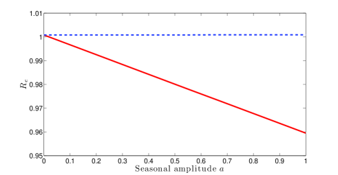
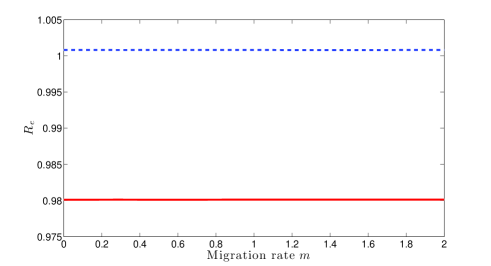
Refer to caption
Refer to caption
Figure 10: Simulations comparing Resubscript𝑅𝑒R_{e} for pulse vaccination (solid) and constant vaccination (dashed) of equal cost for the seasonal version of model (19) with β(t)=β(1+asin(2π(tθ)))𝛽𝑡𝛽1𝑎2𝜋𝑡𝜃\beta(t)=\beta(1+a\sin(2\pi(t-\theta))) and ϕ=0italic-ϕ0\phi=0, so the synchronised pulses occur just before the high-transmission season. The other parameters are f=0𝑓0f=0 and ψ=0.23𝜓0.23\psi=0.23, with the remainder as in Table 1. (a) Resubscript𝑅𝑒R_{e} vs amplitude of seasonality, a𝑎a, with m=0.0𝑚0.0m=0.0 (b) Resubscript𝑅𝑒R_{e} vs m𝑚m with a=0.5𝑎0.5a=0.5.

6.5 Environmental transmission with identical patches and no seasonality

Finally, we consider how environmental transmission affects the results. To begin this section, we state a general theorem about the effective reproduction number for the autonomous (unpulsed) version of the general model (2) with environmental transmission. The following theorem states that the effective reproduction number for the autonomous version of the general model (2) with environmental transmission is identical to the effective reproduction number of the autonomous model (2) without environmental transmission, but with the redefined direct transmission parameter β~ij=βij+ξjνjϵijsubscript~𝛽𝑖𝑗subscript𝛽𝑖𝑗subscript𝜉𝑗subscript𝜈𝑗subscriptitalic-ϵ𝑖𝑗\widetilde{\beta}_{ij}=\beta_{ij}+\frac{\xi_{j}}{\nu_{j}}\epsilon_{ij}.

Refer to caption
Refer to caption
Figure 11: a) Simulations of the system with environmental transmission (18) comparing Resubscript𝑅𝑒R_{e} for pulse vaccination (solid) and constant vaccination (dashed) of equal cost for the single-patch version of model (2) as the fraction of environmental transmission, fesubscript𝑓𝑒f_{e} increases from 0 to 1. The parameters are as in Table 1 with β~=319.655~𝛽319.655\tilde{\beta}=319.655 days-1, ν=5year1𝜈5superscriptyear1\nu=5\ {\rm year}^{-1}, m=f=ec=0𝑚𝑓subscript𝑒𝑐0m=f=e_{c}=0. Note that the parameter values for ξ𝜉\xi and ϵitalic-ϵ\epsilon are absorbed into fesubscript𝑓𝑒f_{e} through a rescaling. b) Resubscript𝑅𝑒R_{e} vs the phase difference, ϕitalic-ϕ\phi, between the vaccination pulses for three different values of fesubscript𝑓𝑒f_{e} (0, 0.2 and 1), when m=1,f=ce=0.1formulae-sequence𝑚1𝑓subscript𝑐𝑒0.1m=1,f=c_{e}=0.1. The rest of the parameters are as in the previous simulation.
Theorem 6.

Denote R^esubscript^𝑅𝑒\widehat{R}_{e} as the effective reproduction number of the autonomous version (2). Let β~ij=βij+ξjνjϵijsubscript~𝛽𝑖𝑗subscript𝛽𝑖𝑗subscript𝜉𝑗subscript𝜈𝑗subscriptitalic-ϵ𝑖𝑗\widetilde{\beta}_{ij}=\beta_{ij}+\frac{\xi_{j}}{\nu_{j}}\epsilon_{ij} and R~esubscript~𝑅𝑒\widetilde{R}_{e} denote the effective reproduction number of the autonomous version of the multi-patch SIR sub-model (no environmental transmission) in (2) with the direct transmission parameter as β~ijsubscript~𝛽𝑖𝑗\widetilde{\beta}_{ij}. Then R^e=R~esubscript^𝑅𝑒subscript~𝑅𝑒\widehat{R}_{e}=\widetilde{R}_{e}.

Proof.

To find the reproduction number, R^esubscript^𝑅𝑒\widehat{R}_{e}, for the autonomous version of (2), we utilize the standard next-generation approach [35]. Then the infection component linearization at the disease-free equilibrium is x˙=(FV)x˙𝑥𝐹𝑉𝑥\dot{x}=(F-V)x, where the 2N×2N2𝑁2𝑁2N\times 2N matrices F𝐹F and V𝑉V can be written in the block-triangular form:

F𝐹\displaystyle F =(DE00),V=(A0BC),formulae-sequenceabsentmatrix𝐷𝐸00𝑉matrix𝐴0𝐵𝐶\displaystyle=\begin{pmatrix}D&E\\ 0&0\end{pmatrix},\quad V=\begin{pmatrix}A&0\\ B&C\end{pmatrix},

in which D,E,A,B,C𝐷𝐸𝐴𝐵𝐶D,E,A,B,C are N×N𝑁𝑁N\times N matrices. Here B𝐵B and C𝐶C are diagonal matrices with ξisubscript𝜉𝑖\xi_{i} and νisubscript𝜈𝑖\nu_{i} (i=1,n𝑖1𝑛i=1,\dots n) as the respective diagonal entries. The entries of matrices D𝐷D, E𝐸E and A𝐴A are as follows: Di,j=βijS¯i,Ei,j=ϵijS¯iformulae-sequencesubscript𝐷𝑖𝑗subscript𝛽𝑖𝑗subscript¯𝑆𝑖subscript𝐸𝑖𝑗subscriptitalic-ϵ𝑖𝑗subscript¯𝑆𝑖D_{i,j}=\beta_{ij}\overline{S}_{i},\ E_{i,j}=\epsilon_{ij}\overline{S}_{i} and Ai,j=(μi+γi+kii)δij+(1δij)(kij)subscript𝐴𝑖𝑗subscript𝜇𝑖subscript𝛾𝑖subscript𝑘𝑖𝑖subscript𝛿𝑖𝑗1subscript𝛿𝑖𝑗subscript𝑘𝑖𝑗A_{i,j}=(\mu_{i}+\gamma_{i}+k_{ii})\delta_{ij}+(1-\delta_{ij})(-k_{ij}), where δijsubscript𝛿𝑖𝑗\delta_{ij} is the Kronecker delta function and S¯=(S¯1,,S¯N)¯𝑆subscript¯𝑆1subscript¯𝑆𝑁\overline{S}=\left(\overline{S}_{1},\dots,\overline{S}_{N}\right) is the disease-free equilibrium. Then

V1=(A10C1BA1C1)and soFV1=(DA1+EC1BA100).formulae-sequencesuperscript𝑉1matrixsuperscript𝐴10superscript𝐶1𝐵superscript𝐴1superscript𝐶1and so𝐹superscript𝑉1matrix𝐷superscript𝐴1𝐸superscript𝐶1𝐵superscript𝐴100V^{-1}=\begin{pmatrix}A^{-1}&0\\ C^{-1}BA^{-1}&C^{-1}\end{pmatrix}\quad\text{and so}\ \ FV^{-1}=\begin{pmatrix}DA^{-1}+EC^{-1}BA^{-1}&*\\ 0&0\end{pmatrix}.

R^esubscript^𝑅𝑒\widehat{R}_{e} is the spectral radius of FV1𝐹superscript𝑉1FV^{-1}, so R^e=ρ(FV1)=ρ((D+EC1B)A1)subscript^𝑅𝑒𝜌𝐹superscript𝑉1𝜌𝐷𝐸superscript𝐶1𝐵superscript𝐴1\widehat{R}_{e}=\rho(FV^{-1})=\rho\left((D+EC^{-1}B)A^{-1}\right). Now define β~ij=βij+ξjνjϵijsubscript~𝛽𝑖𝑗subscript𝛽𝑖𝑗subscript𝜉𝑗subscript𝜈𝑗subscriptitalic-ϵ𝑖𝑗\widetilde{\beta}_{ij}=\beta_{ij}+\frac{\xi_{j}}{\nu_{j}}\epsilon_{ij} and consider the effective reproduction number, R~esubscript~𝑅𝑒\widetilde{R}_{e}, of the autonomous version of (2) with no environmental transmission, but with direct transmission rate β~ijsubscript~𝛽𝑖𝑗\widetilde{\beta}_{ij}. It is not hard to see that R~e=ρ((D+EC1B)A1)subscript~𝑅𝑒𝜌𝐷𝐸superscript𝐶1𝐵superscript𝐴1\widetilde{R}_{e}=\rho\left((D+EC^{-1}B)A^{-1}\right). Thus R^e=R~esubscript^𝑅𝑒subscript~𝑅𝑒\widehat{R}_{e}=\widetilde{R}_{e}, and the result is obtained. ∎

Thus, for the autonomous case, the addition of environmental transmission to an SIR metapopulation model, by considering the system (2), does not qualitatively affect the effective reproduction number. We should note that environmental transmission can result in a substantive delay in epidemic onset and its duration of first peak when compared to the analogous regime of direct transmission [12], so the nature of the transient dynamics is affected by environmental transmission.

For simulations, we include the environmental parameters in the two-patch model (19) and suppose the the patches are identical. Then, using the notation from the previous identical patch case, we can write the infected-component equations as:

dIidt𝑑subscript𝐼𝑖𝑑𝑡\displaystyle\frac{dI_{i}}{dt} =β~Si((1fe)((1f)Ii+fIj)+fe((1ce)Gi+ceGj))(μ+γ)IimIi+mIjabsent~𝛽subscript𝑆𝑖1subscript𝑓𝑒1𝑓subscript𝐼𝑖𝑓subscript𝐼𝑗subscript𝑓𝑒1subscript𝑐𝑒subscript𝐺𝑖subscript𝑐𝑒subscript𝐺𝑗𝜇𝛾subscript𝐼𝑖𝑚subscript𝐼𝑖𝑚subscript𝐼𝑗\displaystyle=\tilde{\beta}S_{i}((1-f_{e})((1-f)I_{i}+fI_{j})+f_{e}((1-c_{e})G_{i}+c_{e}G_{j}))-(\mu+\gamma)I_{i}-mI_{i}+mI_{j} (18)
dGidt𝑑subscript𝐺𝑖𝑑𝑡\displaystyle\frac{dG_{i}}{dt} =ξIiνGi,ij,i,j=1,2,formulae-sequenceabsent𝜉subscript𝐼𝑖𝜈subscript𝐺𝑖formulae-sequence𝑖𝑗𝑖𝑗12\displaystyle=\xi I_{i}-\nu G_{i},\qquad i\neq j,\ i,j=1,2,

where β~β+ξνϵ~𝛽𝛽𝜉𝜈italic-ϵ\tilde{\beta}\equiv\beta+\frac{\xi}{\nu}\epsilon is the total transmission rate, ββ11+β12𝛽subscript𝛽11subscript𝛽12\beta\equiv\beta_{11}+\beta_{12}, ϵϵ11+ϵ12italic-ϵsubscriptitalic-ϵ11subscriptitalic-ϵ12\epsilon\equiv\epsilon_{11}+\epsilon_{12}, feξϵνβ~subscript𝑓𝑒𝜉italic-ϵ𝜈~𝛽f_{e}\equiv\frac{\xi\epsilon}{\nu\tilde{\beta}} is the fraction of environmental transmission, fβ12β𝑓subscript𝛽12𝛽f\equiv\frac{\beta_{12}}{\beta} and ceϵ12ϵsubscript𝑐𝑒subscriptitalic-ϵ12italic-ϵc_{e}\equiv\frac{\epsilon_{12}}{\epsilon} is fraction of cross-transmission for direct and environmental transmission, respectively. Then, by Theorem 6, the effective reproduction number for the autonomous model with constant per capita vaccination rate of susceptibles, σ𝜎\sigma, is

R^e=β~b(μ+σ)(μ+γ).subscript^𝑅𝑒~𝛽𝑏𝜇𝜎𝜇𝛾\displaystyle\widehat{R}_{e}=\frac{\widetilde{\beta}b}{(\mu+\sigma)(\mu+\gamma)}.

Clearly, adding environmental transmission to the identical two-patch model (19) does not alter the autonomous (without pulse vaccination) patch reproduction number R^esubscript^𝑅𝑒\widehat{R}_{e} if we re-define the transmission rate in (17) to be β~~𝛽\widetilde{\beta}.

However, when pulse vaccination is introduced into the model, we find that the fraction of environmental transmission, fesubscript𝑓𝑒f_{e}, affects Resubscript𝑅𝑒R_{e}. In Figure 11, synchronous pulse vaccinations are compared to constant vaccination as fesubscript𝑓𝑒f_{e} is varied. The reproduction number, Resubscript𝑅𝑒R_{e}, under the pulse vaccination shows non-monotone behaviour with respect to fesubscript𝑓𝑒f_{e}, with a maximum occurring around fe=0.2subscript𝑓𝑒0.2f_{e}=0.2 and the minimum occurring at fe=1subscript𝑓𝑒1f_{e}=1 (where all of the transmission is due to the environment). We remark that this graph looks the same for many different values that we utilised for the migration rate and cross transmission, in particular for the case of isolated patches. The other parameters are as in Table 1 with β~=319.655~𝛽319.655\tilde{\beta}=319.655 days-1 and ν=5year1𝜈5superscriptyear1\nu=5\ {\rm year}^{-1}. Note that the parameter values for ξ𝜉\xi and ϵitalic-ϵ\epsilon are absorbed into fesubscript𝑓𝑒f_{e} through a rescaling. Of course, we know from before that when fe=0subscript𝑓𝑒0f_{e}=0, the vaccination strategies yield identical Resubscript𝑅𝑒R_{e} (proven in the isolated patch case without seasonality). In contrast, even in the single patch case, environmental transmission can cause disagreement in the reproduction numbers for pulse- and constant-vaccination strategies of equal cost. This result can be viewed as an impulsive analogue to that showing that sinusoidal transmission alters the reproduction number for an SEIR model, but leaves the reproduction number for the SIR model the same as with constant transmission [6, 13]. Indeed, an SEIR model can be seen as a special case of the no-impulse environmental transmission model. In Figure 11, we vary the phase difference, ϕitalic-ϕ\phi, between the vaccination pulses for three different values of fesubscript𝑓𝑒f_{e} (0, 0.2 and 1), when m=1,f=ce=0.1formulae-sequence𝑚1𝑓subscript𝑐𝑒0.1m=1,f=c_{e}=0.1. The remaining parameters are as in Table 1.

7 Discussion

We have studied pulse vaccination in metapopulations, using poliovirus vaccination as our focus. By allowing each patch to have distinct, periodic pulse-vaccination schedules connected with a common period — along with considering seasonality, environmental transmission and two types of mobility — we add more generality and complexity to prior models. The effective reproduction number, Resubscript𝑅𝑒R_{e}, is defined for the model, system (2), and found to be a global threshold. If Re<1subscript𝑅𝑒1R_{e}<1, then the disease dies out; on the other hand, when Re>1subscript𝑅𝑒1R_{e}>1, the disease uniformly persists.

Through theoretical analysis and numerical simulations, we were able to gain insights into optimising vaccination strategies in the metapopulation setting. Theorem 5 and the supporting numerical simulations show that synchronising vaccination pulses among connected patches is key in minimising the effective reproduction number. An open problem is to analytically prove that synchronising the pulses minimises Resubscript𝑅𝑒R_{e} under more general conditions than are assumed in Theorem 5.

Evidence from the epidemiological data suggests that pulse synchronisation at different spatial scales influences the effectiveness of a vaccination campaign. Based on field studies, the WHO recommends that the duration of the vaccination campaign, in the form of national immunisation days, be as short as possible (1–2 days) [10]. The importance of administering the vaccine across a whole country in 1–2 days, as opposed to taking a longer period of time, may be in part due to the higher levels of synchronisation for the shorter duration vaccination campaign. Increased seroconversion rates also seem to play a role in the optimality of mass vaccinations with short duration [10]. On an international scale, the effectiveness of Operation MECACAR [37] and a study of the effect of migration on measles incidence after mass vaccination in Burkina Faso [41] point to the importance of pulse synchronisation. Our study highlights the critical role that the WHO and national governments can play in optimising disease control by synchronising mass vaccination campaigns among countries and regions.

Another important problem is comparing the effectiveness of periodic mass (pulse) vaccination versus routine (constant) vaccination. Disease-control authorities must consider certain logistical aspects, which may affect the cost of implementing a particular strategy. From a mathematical perspective, the fundamental starting point for comparison is to consider Resubscript𝑅𝑒R_{e} for strategies of equal vaccinations per period. For the case of no seasonality and environmental transmission, we find some cases where the strategies are equivalent in terms of Resubscript𝑅𝑒R_{e}. When seasonality is included, a well-timed pulse-vaccination strategy (simultaneous pulses administered during the season before the high-transmission season) is optimal (assuming the patches have synchronous seasons), similar to results for the single-patch SIR model [29]. Future work will consider comparing pulse vaccination and constant-vaccination strategies in a stochastic model, which yields some insights not seen in the deterministic setting.

More work needs to be done in the case of environmental transmission. When indirect transmission was considered to be a major mode of transmission in other studies, a delay in epidemic onset and its extension when compared to the analogous regime of direct transmission were observed [12]. This could be explained by the persistence of the virus in the environment leading to new infections generated over a longer duration than that of the direct contact. Such a two-step mechanism, with a human-to-environment segment and an environment-to-human segment, could lead to delay and extension of the effective infectious period when compared to that of direct human-to-human transmission [12]. Interestingly, we found that varying the fraction of environmental transmission in the system alters the effective reproduction number Resubscript𝑅𝑒R_{e} under pulse vaccination, contrary to results for the case of constant-rate vaccination. Further consideration of the interaction of environment-induced delay with the influence of seasonality on environmental transmission and pulse vaccination is the subject of our ongoing work.

Finally, we mention the importance of incorporating mobility and spatial structure into disease models. In addition to our findings about the how mobility induces an advantage to synchronise pulse vaccination, population movement has other implications for disease control. As found in previous work on autonomous models [31], imbalance in migration rates among the patches can have a large effect on the overall reproduction number, which may alter the optimal vaccine distribution among patches or may influence disease-control strategies related to movement restriction. The combination of population movement with complexities of control strategies and disease transmission presents many problems for which mathematical modelling may yield valuable insight.

Acknowledgements

We are grateful to two anonymous reviewers whose comments greatly improved the manuscript. RJS? is supported by an NSERC Discovery Grant. For citation purposes, note that the question mark in “Smith?” is part of his name.

References

  • [1]
  • [2] Agur, Z., L. Cojocaru, G. Mazor, R. Anderson, Y. Danon (1993). Pulse mass measles vaccination across age cohorts. Proc. Natl. Acad. Sci. 90:11698–11702
  • [3] Alyward, B., K.A. Hennessey, N. Zagario, J.-M.Olivé and S. Cochi (2000). When Is a Disease Eradicable? 100 Years of Lessons Learned. American Journal of Public Health 90:10, 1515–1520.
  • [4] Bacaer, N. and E.H. Ait Dads (2012). On the biological interpretation of a definition for the parameter R0subscript𝑅0R_{0} in periodic population models. J. Math. Biol. 65:601–621.
  • [5] Bacaer, N. and S. Guernaoui-Morocco (2006). The epidemic threshold of vector-borne diseases with seasonality. The case of cutaneous leishmaniasis in Chichaoua. J. Math. Biol. 53:421–436.
  • [6] Bacaër, N. and R. Ouifki (2007). Growth rate and basic reproduction number for population models with a simple periodic factor, Math. Biosci., 210:647–658.
  • [7] Bainov, D.D., Simeonov, P.S. (1989). Systems with Impulsive Effect. Ellis Horwood Ltd, Chichester.
  • [8] Bainov, D.D., Simeonov, P.S. (1993). Impulsive differential equations: periodic solutions and applications. Longman Scientific and Technical, Burnt Mill.
  • [9] Bainov, D.D., Simeonov, P.S. (1995). Impulsive Differential Equations: Asymptotic Properties of the Solutions. World Scientific, Singapore.
  • [10] Birmingham, M.E., R.B. Aylward, S.L. Cochi and H.F. Hull (1997). National immunization days: state of the art. J. Infect. Dis. 175:S183–188.
  • [11] Breban, R., J. Drake, D.E. Stallknecht, P. Rohani (2009). The Role of Environmental Transmission in Recurrent Avian Influenza Epidemics. PLoS Comput Biol 5(4): e1000346.
  • [12] Bourouiba, L., Teslya, S. L., and Wu, J. (2011) Highly pathogenic avian influenza outbreak mitigated by seasonal low pathogenic strains: Insights form dynamic modeling. J. Theor. Biol. 271: 181-201.
  • [13] Browne, C.J. and S.S. Pilyugin (2012). Periodic Multidrug Therapy in a Within-Host Virus Model, Bull. Math. Biol., 74:562–589.
  • [14] Burton, J., L. Billings, D.A.T. Cummings and I.B. Schwartz (2012). Disease persistence in epidemiological models: The interplay between vaccination and migration. Math. Biosci., 239(1):91–96.
  • [15] C.C. Chicone, Ordinary Differential Equations With Applications, 2nd edition, Springer, New York, 2006.
  • [16] Earn, D.J.D., P. Rohani and B.T. Grenfell (1998). Persistence, chaos, and synchronicity in ecology and epidemiology, Proc. R. Soc. Lond.-B, 265:7–10.
  • [17] Fine, P.E.M. and I.A.M. Carneiro (1999). Transmissibility and persistence of oral polio vaccine viruses: implications for the global poliomyelitis eradication initiative. American Journal of Epidemiology 150(10): 1001–1021.
  • [18] Heffernan, J.M., R.J. Smith and L.M. Wahl (2005). Perspectives on the basic reproductive ratio. J. R. Soc. Interface, 2(4):281–293.
  • [19] Kealey, A.D. and R.J. Smith? (2010). Neglected Tropical Diseases: Infection, Modeling, and Control. J. Health Care Poor Underserved 21:53–69.
  • [20] Kirkilionis, M. and S. Walcher (2004). On comparison systems for ordinary differential equations. J Math Anal Appl 299:157–173.
  • [21] Li J., D. Blakeley and R.J. Smith? (2011). The Failure of R0subscript𝑅0R_{0}. Comp. Math. Methods Med., Vol. 2011, Article ID 527610.
  • [22] Liebovitch, L.S. and I.B. Schwartz (2004). Migration induced epidemics: dynamics of flux based multipatch models, Physics Letters A 332:256–267.
  • [23] Liu J. and Y. Zhou (2009). Global stability of an SIRS epidemic model with transport related infection, Chaos, Solitons & Fractals 40(1):145–158.
  • [24] Lloyd, A.L. and V.A.A. Jansen (2004). Spatiotemporal dynamics of epidemics: synchrony in metapopulation models, Mathematical Biosciences 188 1–16.
  • [25] V. Lakshmikantham, D. Bainov, and P. Simeonov, Theory of Impulsive Differential Equations, World Scientific, Singapore, 1989.
  • [26] Losos J. Report of the work group on viral diseases. In:Goodman RA, Foster KL, Trowbridge FL, Figueroa JP, eds. Global disease elimination and eradication as public health strategies. Bull World Health Organ. 1998;76(suppl2):94–102.
  • [27] Meng, X., L. Chen and B. Wu (2010). A delay SIR epidemic model with pulse vaccination and incubation times. Nonlinear Analysis: Real World Applications 11(1):88–98.
  • [28] Morens, D.M., E.C. Holmes, A.S. Davis and J.K. Taunbenberger (2011). Global Rinderpest Eradication: Lessons Learned and Why Humans Should Celebrate Too. J Infect Dis. 204(4):502–505.
  • [29] Onyango, N.O. and J. Müller (2013). Determination of optimal vaccination strategies using an orbital stability threshold from periodically driven systems. J. Math. Biol. (in press)
  • [30] Smith?, R.J., P. Cloutier, J. Harrison and A. Desforges (2012). A mathematical model for the eradication of Guinea Worm Disease. In: Understanding the dynamics of emerging and re-emerging infectious diseases using mathematical models, S. Mushayabasa and C.P. Bhunu, eds, pp133–156.
  • [31] Smith?, R.J., J. Li, R. Gordon, J.M. Heffernan (2009). Can we spend our way out of the AIDS epidemic? A world halting AIDS model. BMC Public Health 9(Suppl 1):S15.
  • [32] Shulgin, B., L. Stone and Z. Agur (1998). Pulse vaccination strategy in the SIR epidemic model. Bull. Math. Biol. 60:1123–1148.
  • [33] Terry, A.J. (2010). Pulse vaccination strategies in a metapopulation SIR model, Math. Biosci. Eng. 7:457–479.
  • [34] H.R. Thieme, Mathematics in Population Biology, Princeton University Press, Princeton 2003.
  • [35] van den Driessche, P., Watmough, J. 2002. Reproduction numbers and sub-threshold endemic equilibria for compartmental models of disease transmission. Math. Biosci. 180, 29–48.
  • [36] Wang, W. and X.-Q. Zhao (2008). Threshold dynamics for compartmental epidemic models in periodic environments. J. Dyn. Differ. Equ. 20:699–717.
  • [37] World Health Organization Regional Offices for Europe and the Eastern Mediterranean. Operation MECACAR: eradicating polio, final report 1995–2000. Copenhagen, Denmark: World Health Organization Regional Office for Europe, 2001.
  • [38] World Health Organization. The case for completing polio eradication. Geneva, Switzerland: World Health Organization, 2008. Available at: http://www.polioeradication.org/content/publications/thecase_final.pdf
  • [39] Xiao, Y., S. Tang, Y. Zhou, R.J. Smith?, J. Wu and N. Wang (2013). Predicting an HIV/AIDS epidemic and measuring the effect of mobility in mainland China. Journal of Theoretical Biology, 317, 271–285.
  • [40] Xiao, Y. and X. Zou (2013). Transmission dynamics for vector-borne diseases in a patchy environment. J. Math. Biol. (in press).
  • [41] Yameogo, K.R., R.T. Perry, A. Yameogo, et al. (2005) Migration as a risk factor for measles after a mass vaccination campaign, Burkina Faso, 2002. Int. J. Epidemiol. 34, 556–564.
  • [42] Yang, Y.P. and Y.N. Xiao (2010). The effects of population dispersal and pulse vaccination on disease control. Math. Comput. Model. 52:1591–1604.
  • [43] X.-Q. Zhao, Dynamical Systems in Population Biology, Springer, New York, 2003.
  • [44] Zipursky, S., L. Boualam, D.O. Cheikh, J. Fournier-Caruana, D. Hamid, M. Janssen, U. Kartoglu, G. Waeterloos and O. Ronveaux (2011). Assessing the potency of oral polio vaccine kept outside of the cold chain during a national immunization campaign in Chad. Vaccine 29(34):5652–5656.