The Galerkin Method for Perturbed Self-Adjoint Operators and Applications

Abstract.

We consider the Galerkin method for approximating the spectrum of an operator $T+A$ where $T$ is semi-bounded self-adjoint and $A$ satisfies a relative compactness condition. We show that the method is reliable in all regions where it is reliable for the unperturbed problem - which always contains $\mathbb{C}\backslash\mathbb{R}$. The results lead to a new technique for identifying eigenvalues of $T$, and for identifying spectral pollution which arises from applying the Galerkin method directly to $T$. The new technique benefits from being applicable on the form domain.

Keywords Eigenvalue problem, spectral pollution, Galerkin method, finite-section method.

2010 Mathematics Subject Classification 47A55, 47A58.

¹WIMCS-Leverhulme Fellow, School of Mathematics, Cardiff University, Senghennydd Road, CARDIFF CF24 4AG, Wales, UK. straussmd@cardiff.ac.uk.

1. Introduction

In general, the approximation of the spectrum of a semi-bounded self-adjoint a operator $T$ with the Galerkin (finite section) method is reliable only for those eigenvalues lying below the essential spectrum. Any element from the closed convex hull of $\sigma_{\mathrm{ess}}(T)\cup\{\infty\}$ can in principle be the limit point of a sequence of Galerkin eigenvalues; see [12, Theorem 2.1]. This phenomenon is called spectral pollution and constitutes a serious problem in computational spectral theory; see for example [1, 2, 6, 15]. As is well-known, under fairly mild assumptions on a sequence of trial spaces the Galerkin method will capture the whole spectrum, although eigenvalues may be obscured by spectral pollution. In the presence of essential spectrum, the Galerkin method applied to non-self-adjoint operators is less well understood. Reliability of the Galerkin method is assured in some situations, notably for compact operators or operators with compact resolvent and satisfying ellipticity conditions; see for example [5] and reference therein.

The closed sesquilinear form associated to $T$ we denote by $\mathfrak{t}$. Let $A$ be a closed, $|T|^{\frac{1}{2}}$-compact operator, such that $(T+A)^{*}=T+A^{*}$ and for some $0\leq\alpha<1$, $\beta\geq 0$ satisfies

(1.1) $$|\langle A\phi,\phi\rangle|\leq\alpha\mathfrak{t}[\phi]+\beta\|\phi\|^{2}\quad\textrm{for all}\quad\phi\in{\rm Dom}(\mathfrak{t})={\rm Dom}(|T|^{\frac{1}{2}}).$$

We note that $\sigma_{\mathrm{ess}}(T+A)=\sigma_{\mathrm{ess}}(T)$; see for example [11, Theorem IV.5.35]. In Section 2 we shall be concerned with the approximation of the discrete spectrum (isolated eigenvalues of finite multiplicity) of $T+A$ by means of the Galerkin method. In Theorem 2.3 we show that if a compact set $\Gamma\subset\rho(T+A)$ does not contain a limit point of Galerkin eigenvalues for the self-adjoint operator $T$ and sequence of trial spaces $(\mathcal{L}_{n})$, then $\Gamma$ will not contain a limit point of Galerkin eigenvalues for the operator $T+A$. Further, if in a region $U\subset\mathbb{C}$ with $U\cap\sigma_{\mathrm{ess}}(T)=\varnothing$, the self-adjoint operator $T$ does not suffer from spectral pollution for a sequence of trial spaces $(\mathcal{L}_{n})$, then Theorem 2.5 states that $\sigma(T+A)\cap U$ will be approximated and without spectral pollution, and by Theorem 2.9 the Galerkin method will also capture the multiplicity of eigenvalues in the region.

In Section 3 we employ the preceding results to aid the development of a new technique for approximating those eigenvalues of $T$ which lie within the closed convex hull of $\sigma_{\mathrm{ess}}(T)\cup\{\infty\}$ - the region where a direct application of the Galerkin method is unreliable. This is an issue which has received considerable attention in recent decades. There are two approaches to the problem. Firstly, general methods which may be applied to an arbitrary self-adjoint operator, and secondly, methods designed for a specific class of operator. Examples of the former are proposed in [8, 12, 16, 18] and can be highly effective. However, application of these techniques can require a priori information about the spectrum, and always require trial subspaces to belong to the operator domain rather than the preferred form domain. The latter is due to requiring matrices with entries of the form $\langle T\phi,T\psi\rangle$, while the Galerkin method requires only matrices with entries of the form $\mathfrak{t}(\phi,\psi)$. A new method designed for a specific class of operator is studied in [13, 14] and is applicable to operators of the form $T=-\Delta+q$ which act on $L^{2}(\mathbb{R}^{n})$ and $L^{2}(0,\infty)$, respectively. The idea is to apply the Galerkin method to the perturbed operator $-\Delta+q+is$ for a suitably chosen function $s$. The result of the perturbation is to lift eigenvalues of $T$ off the real line where they can be approximated without encountering spectral pollution. Based on this idea and using the form domain, we consider the Galerkin method applied to $T+iQ$ where $Q$ is an orthogonal projection. For a set $J\subset\mathbb{R}$ and a trial space $\mathcal{L}$ we choose $Q$ to be the orthogonal projection onto the eigenspace associated to Galerkin eigenvalues contained in $J$, we then apply the Galerkin method to $T+iQ$ and a larger trial space. In Theorem 3.6 we show that if $\lambda\in\sigma_{\mathrm{dis}}(T)\cap J$ and our trial space $\mathcal{L}$ approximates the corresponding eigenspace sufficiently well, then $T+iQ$ will have eigenvalues in a neighbourhood of $\lambda+i$ with total-multiplicity equally that of $\lambda\in\sigma_{\mathrm{dis}}(T)$. Now applying results from Section 2, we may approximate the non-real eigenvalues of $T+iQ$, their multiplicities, and free from spectral pollution. The technique is effectively applied to examples where eigenvalues are obscured by spectral pollution.

2. The Truncated Eigenvalue Problem

We set $m=\min\sigma(T)$ and denote by $\mathcal{H}_{\mathfrak{t}}$ the Hilbert space ${\rm Dom}(\mathfrak{t})$ equipped with the inner product

$$\langle\phi,\psi\rangle_{\mathfrak{t}}:=(\mathfrak{t}-m)(\phi,\psi)+\langle\phi,\psi\rangle\quad\textrm{and norm}\quad\|\phi\|_{\mathfrak{t}}^{2}:=(\mathfrak{t}-m)[\phi]+\|\phi\|^{2}.$$

Throughout, $(\mathcal{L}_{n})\subset{\rm Dom}(\mathfrak{t})$ is a sequence of finite-dimensional subspaces. The orthogonal projections from $\mathcal{H}$ and $\mathcal{H}_{\mathfrak{t}}$ onto $\mathcal{L}_{n}$ will be denoted by $P_{n}$ and $\hat{P}_{n}$, respectively. We always assume that the sequence $(\mathcal{L}_{n})$ is dense in $\mathcal{H}_{\mathfrak{t}}$:

$$\forall\phi\in{\rm Dom}(\mathfrak{t})\quad\exists\phi_{n}\in\mathcal{L}_{n}:\quad\|\phi-\phi_{n}\|_{\mathfrak{t}}\to 0.$$

We define the form

$$\mathfrak{s}(\phi,\psi):=\mathfrak{t}(\phi,\psi)+\langle A\phi,\psi\rangle\quad\textrm{with}\quad{\rm Dom}(\mathfrak{s})={\rm Dom}(\mathfrak{t}),$$

the sets

$$\sigma(T+A,\mathcal{L}_{n}) :=\{z\in\mathbb{C}:~{}\exists\phi\in\mathcal{L}_{n}\quad\textrm{with}\quad\mathfrak{s}(\phi,\psi)=z\langle\phi,\psi\rangle~{}\forall\psi\in\mathcal{L}_{n}\}$$

$$\sigma(T,\mathcal{L}_{n}) :=\{z\in\mathbb{C}:~{}\exists\phi\in\mathcal{L}_{n}\quad\textrm{with}\quad\mathfrak{t}(\phi,\psi)=z\langle\phi,\psi\rangle~{}\forall\psi\in\mathcal{L}_{n}\},$$

and the limit sets

$$\sigma(T+A,\mathcal{L}_{\infty}) :=\{z\in\mathbb{C}:~{}\exists~{}z_{n}\in\sigma(T+A,\mathcal{L}_{n})\textrm{ with }z_{n}\to z\}$$

$$\sigma(T,\mathcal{L}_{\infty}) :=\{z\in\mathbb{C}:~{}\exists~{}z_{n}\in\sigma(T,\mathcal{L}_{n})\textrm{ with }z_{n}\to z\}.$$

Associated to the restriction of $\mathfrak{s}$ and $\mathfrak{t}$ to $\mathcal{L}_{n}$ are operators $S_{n}$ and $T_{n}$ which act on the Hilbert space $\mathcal{L}_{n}$, and satisfy

$$\langle S_{n}\phi,\psi\rangle=\mathfrak{s}(\phi,\psi)\quad\textrm{and}\quad\langle T_{n}\phi,\psi\rangle=\mathfrak{t}(\phi,\psi).$$

Evidently, we have $\sigma(T+A,\mathcal{L}_{n})=\sigma(S_{n})$ and $\sigma(T,\mathcal{L}_{n})=\sigma(T_{n})$.

2.1. Regular Sets

We say that $\Gamma\subset\mathbb{C}$ is a $T_{n}$-regular set if there exist a $\delta>0$ and $N\in\mathbb{N}$, with

(2.1) $$\min_{\genfrac{}{}{0.0pt}{}{\phi\in\mathcal{L}_{n}}{\|\phi\|=1}}\max_{\genfrac{}{}{0.0pt}{}{\psi\in\mathcal{L}_{n}}{\|\psi\|=1}}|(\mathfrak{t}-z)(\phi,\psi)|\geq\delta\quad\textrm{for all}\quad z\in\Gamma,\quad\textrm{and}\quad n\geq N,$$

or equivalently

(2.2) $$\|(T_{n}-z)\phi\|\geq\delta\|\phi\|\quad\textrm{for all}\quad z\in\Gamma,\quad\phi\in\mathcal{L}_{n}\quad\textrm{and}\quad n\geq N.$$

Similarly, we define $S_{n}$-regular sets, and we shall make use of the function

$$\sigma_{n}(z) :=\min_{\genfrac{}{}{0.0pt}{}{\phi\in\mathcal{L}_{n}}{\|\phi\|=1}}\max_{\genfrac{}{}{0.0pt}{}{\psi\in\mathcal{L}_{n}}{\|\psi\|=1}}|(\mathfrak{s}-z)(\phi,\psi)|$$

$$=\min_{\genfrac{}{}{0.0pt}{}{\phi\in\mathcal{L}_{n}}{\|\phi\|=1}}\|(S_{n}-z)\phi\|$$

$$=\begin{cases}\|(S_{n}-z)^{-1}\|^{-1}&\text{if }z\in\rho(S_{n}),\\[4.30554pt] 0&\text{if }z\in\sigma(S_{n}).\end{cases}$$

Lemma 2.1.

If $\Gamma$ is a $T_{n}$-regular set, then $\Gamma\subset\rho(T)$.

Proof.

We suppose the contrary, so that $\Gamma$ is a $T_{n}$-regular set and $\lambda\in\Gamma\cap\sigma(T)$. There exists a normalised sequence $(\psi_{k})\subset{\rm Dom}(T)$ such that $\|(T-\lambda)\psi_{k}\|<k^{-1}$. For a fixed $k$, let $\hat{\psi}_{n}=\hat{P}_{n}\psi_{k}$. Then for any normalised $v_{n}\in\mathcal{L}_{n}$ we have

$$|\mathfrak{t}(\hat{\psi}_{n},v_{n})-\lambda\langle\hat{\psi}_{n},v_{n}\rangle| =|\mathfrak{t}(\hat{\psi}_{n}-\psi_{k},v_{n})+\mathfrak{t}(\psi_{k},v_{n})-\lambda\langle\hat{\psi}_{n},v_{n}\rangle|$$

$$=|\langle\hat{\psi}_{n}-\psi_{k},v_{n}\rangle_{\mathfrak{t}}+(m-1)\langle\hat{\psi}_{n}-\psi_{k},v_{n}\rangle$$

$$\qquad+\langle(T-\lambda)\psi_{k},v_{n}\rangle-\lambda\langle\hat{\psi}_{n}-\psi_{k},v_{n}\rangle|$$

$$=|\langle(\hat{P}_{n}-I)\psi_{k},v_{n}\rangle_{\mathfrak{t}}+\langle(T-\lambda)\psi_{k},v_{n}\rangle$$

$$\qquad-(\lambda-m+1)\langle\hat{\psi}_{n}-\psi_{k},v_{n}\rangle|$$

$$=|\langle(T-\lambda)\psi_{k},v_{n}\rangle-(\lambda-m+1)\langle\hat{\psi}_{n}-\psi_{k},v_{n}\rangle|$$

$$<k^{-1}+|\lambda-m+1|\|\hat{\psi}_{n}-\psi_{k}\|,$$

where the right hand side is less than $k^{-1}$ for all sufficiently large $n$. Since $\|\hat{\psi}_{n}\|\to 1$ it follows that $\Gamma$ is not a $T_{n}$-regular set. The result follows from the contradiction. ∎

Lemma 2.2.

Let $(\phi_{n})$ be a bounded sequence of vectors with $\phi_{n}\in\mathcal{L}_{n}$ and

$$\max_{\genfrac{}{}{0.0pt}{}{v\in\mathcal{L}_{n}}{\|v\|=1}}|(\mathfrak{s}-z)(\phi_{n},v)-\langle x,v\rangle|\to 0\quad\textrm{as}\quad n\to\infty.$$

There exists a $u\in\mathcal{H}$ and a subsequence $n_{k}$, such that $\|A\phi_{n_{k}}-u\|\to 0$. Moreover, if $\{z\}$ is a $T_{n}$-regular set, then $\|\phi_{n_{k}}-(T-z)^{-1}(x-u)\|_{\mathfrak{t}}\to 0$.

Proof.

Suppose that $A\phi_{n}$ does not have a convergent subsequence. It follows that $\||T|^{\frac{1}{2}}\phi_{n}\|\to\infty$ and therefore also that $\mathfrak{t}[\phi_{n}]\to\infty$. We have

$$\langle x,\phi_{n}\rangle\approx(\mathfrak{s}-z)(\phi_{n},\phi_{n})=\mathfrak{t}[\phi_{n}]+\langle A\phi_{n},\phi_{n}\rangle-z\langle\phi_{n},\phi_{n}\rangle.$$

Let $M\in\mathbb{R}$ be such that $\|\phi_{n}\|\leq M$ for all $n\in\mathbb{N}$. Using (1.1) and recalling that $m=\min\sigma(T)$, we obtain

$$\mathfrak{t}[\phi_{n}] \approx z\langle\phi_{n},\phi_{n}\rangle-\langle A\phi_{n},\phi_{n}\rangle+\langle x,\phi_{n}\rangle$$

$$\leq|z|M^{2}+|\langle A\phi_{n},\phi_{n}\rangle|+\|x\|M$$

$$\leq|z|M^{2}+\alpha\langle|T|\phi_{n},\phi_{n}\rangle+\beta M^{2}+\|x\|M$$

$$\leq|z|M^{2}+\alpha\mathfrak{t}[\phi_{n}]+2\alpha|m|M^{2}+\beta M^{2}+\|x\|M.$$

Therefore

$$\mathfrak{t}[\phi_{n}]\leq\frac{|z|M^{2}+2\alpha|m|M^{2}+\beta M^{2}+\|x\|M}{1-\alpha}$$

which is a contradiction since the left hand side converges to $\infty$. We deduce that $A\phi_{n_{k}}\to u$ for some $u\in\mathcal{H}$ and subsequence $n_{k}$.

Suppose now that $\{z\}$ is a $T_{n}$-regular set. Then by Lemma 2.1 we have $z\in\rho(T)$, hence there exists a vector $\psi\in{\rm Dom}(T)$ with $(T-z)\psi=x-u$. Let $\psi_{n}=\hat{P}_{n}\psi$, then for any normalised $v_{n}\in\mathcal{L}_{n}$ we have

$$\mathfrak{t}(\psi_{n},v_{n})-z\langle\psi_{n},v_{n}\rangle =\mathfrak{t}(\psi,v_{n})-z\langle\psi,v_{n}\rangle+\mathfrak{t}(\psi_{n}-\psi,v_{n})-z\langle\psi_{n}-\psi,v_{n}\rangle$$

$$=\langle(T-z)\psi,v_{n}\rangle+(\mathfrak{t}-m)(\psi_{n}-\psi,v_{n})+\langle\psi_{n}-\psi,v_{n}\rangle$$

$$\qquad-(z-m+1)\langle\psi_{n}-\psi,v_{n}\rangle$$

$$=\langle x-u,v_{n}\rangle+\langle\psi_{n}-\psi,v_{n}\rangle_{\mathfrak{t}}-(z-m+1)\langle\psi_{n}-\psi,v_{n}\rangle$$

$$=\langle x-u,v_{n}\rangle+\langle(\hat{P}_{n}-I)\psi,v_{n}\rangle_{\mathfrak{t}}-(z-m+1)\langle\psi_{n}-\psi,v_{n}\rangle$$

$$=\langle x-u,v_{n}\rangle-(z-m+1)\langle\psi_{n}-\psi,v_{n}\rangle$$

and

$$\mathfrak{t}(\phi_{n},v_{n})+\langle A\phi_{n},v_{n}\rangle-z\langle\phi_{n},v_{n}\rangle=(\mathfrak{s}-z)(\phi_{n},v_{n})\approx\langle x,v_{n}\rangle.$$

Hence, we have

$$\mathfrak{t}(\phi_{n_{k}},v_{n_{k}})-z\langle\phi_{n_{k}},v_{n_{k}}\rangle\approx\langle x-u,v_{n_{k}}\rangle$$

and

$$\mathfrak{t}(\phi_{n_{k}}-\psi_{n_{k}},v_{n_{k}})-z\langle\phi_{n_{k}}-\psi_{n_{k}},v_{n_{k}}\rangle\to 0.$$

Since $\{z\}$ is a $T_{n}$-regular set we deduce that $\phi_{n_{k}}-\psi_{n_{k}}$ and $\mathfrak{t}(\phi_{n_{k}}-\psi_{n_{k}},v_{n_{k}})$ both converge to zero. In particular, we have $\mathfrak{t}[\phi_{n_{k}}-\psi_{n_{k}}]\to 0$, and therefore $\|\phi_{n_{k}}-\psi_{n_{k}}\|_{\mathfrak{t}}\to 0$, hence

$$\|\phi_{n_{k}}-\psi\|_{\mathfrak{t}} \leq\|\phi_{n_{k}}-\psi_{n_{k}}\|_{\mathfrak{t}}+\|\psi_{n_{k}}-\psi\|_{\mathfrak{t}}$$

$$=\|\phi_{n_{k}}-\psi_{n_{k}}\|_{\mathfrak{t}}+\|(\hat{P}_{n_{k}}-I)\psi\|_{\mathfrak{t}}$$

$$\to 0.$$

∎

Theorem 2.3.

Let $\Gamma\subset\mathbb{C}$ be a compact $T_{n}$-regular set. If $\Gamma\subseteq\rho(T+A)$ then $\Gamma$ is an $S_{n}$-regular set.

Proof.

Suppose the assertion is false. Then there exists a subsequence $n_{k}$ and a sequence $(z_{n_{k}})\subset\Gamma$, such that $\sigma_{n_{k}}(z_{n_{k}})\to 0$ as $k\to\infty$. We assume without loss of generality that $\sigma_{n}(z_{n})\to 0$ for some sequence $(z_{n})\subset\Gamma$. Since $\Gamma$ is a compact set it follows that $(z_{n})$ has a convergent subsequence, and without loss of generality we assume that $z_{n}\to z\in\Gamma$. Therefore, for a sequence of normalised vectors $\phi_{n}\in\mathcal{L}_{n}$ we have

$$\max_{\genfrac{}{}{0.0pt}{}{v\in\mathcal{L}_{n}}{\|v\|=1}}|(\mathfrak{s}-z)(\phi_{n},v)|\to 0\quad\textrm{as}\quad n\to\infty.$$

By Lemma 2.2 there exists a $u\in\mathcal{H}$ and subsequence $n_{k}$ with

$$\|A\phi_{n_{k}}-u\|\to 0\quad\textrm{and}\quad\|\phi_{n_{k}}+(T-z)^{-1}u\|_{\mathfrak{t}}\to 0.$$

Without loss of generality we assume that

$$\|A\phi_{n}-u\|\to 0\quad\textrm{and}\quad\|\phi_{n}+(T-z)^{-1}u\|_{\mathfrak{t}}\to 0.$$

We note that $u\neq 0$. We have $z\in\rho(T+A)$ and therefore $\overline{z}\in\rho(T+A^{*})$. Let $\psi\in{\rm Dom}(T+A^{*})$ be such that $(T+A^{*}-\overline{z})\psi=-(T-z)^{-1}u$. Set $\psi_{n}=\hat{P}_{n}\psi$, then $\|\psi_{n}-\psi\|_{\mathfrak{t}}\to 0$, hence $\mathfrak{t}(\phi_{n},\psi_{n})\to-\mathfrak{t}((T-z)^{-1}u,\psi)$ (see [11, Theorem VI.1.12]). We obtain

$$0 \leftarrow(\mathfrak{s}-z)(\phi_{n},\psi_{n})$$

$$=\mathfrak{t}(\phi_{n},\psi_{n})+\langle A\phi_{n},\psi_{n}\rangle-z\langle\phi_{n},\psi_{n}\rangle$$

$$\to-\mathfrak{t}((T-z)^{-1}u,\psi)-\langle A(T-z)^{-1}u,\psi\rangle+z\langle(T-z)^{-1}u,\psi\rangle$$

$$=-\langle(T-z)^{-1}u,T\psi\rangle-\langle(T-z)^{-1}u,A^{*}\psi\rangle+z\langle(T-z)^{-1}u,\psi\rangle$$

$$=-\langle(T-z)^{-1}u,(T+A^{*}-\overline{z})\psi\rangle$$

$$=\|(T-z)^{-1}u\|^{2},$$

however, the right hand side is non-zero. From the contradiction we deduce that $\Gamma$ is an $S_{n}$-regular set. ∎

2.2. Uniform Sets

We say that an open set $U\subseteq\mathbb{C}$ is a $T_{n}$-uniform set if:

• any compact subset of $U\cap\rho(T)$ is $T_{n}$-regular

• $U\cap\sigma(T,\mathcal{L}_{\infty})=U\cap\sigma(T)\subset\sigma_{\mathrm{dis}}(T)$

• if $\lambda\in\sigma(T)\cap U$ and $\Gamma\subset U$ is a circle with center $\lambda$ and which neither intersects nor encloses any other element from $\sigma(T)$, then for all sufficiently large $n$ the total multiplicity of those eigenvalues of $T_{n}$ enclosed by $\Gamma$ equals the multiplicity of the eigenvalue $\lambda$.
  

$U$ is assumed to be a $T_{n}$-uniform set for the remainder of this section. For a $\lambda\in\sigma(T)\cap U$ we denote the corresponding spectral subspace by $\mathcal{L}(\{\lambda\})$. Let $\Gamma\subset U$ be a circle with center $\lambda$ and which neither intersects nor encloses any other element from $\sigma(T)$. We denote by $\mathcal{L}_{n}(\Gamma)$ the spectral subspace associated to those elements from $\sigma(T,\mathcal{L}_{n})$ which are enclosed by $\Gamma$.

We use the following notions of the gap between subspaces $\mathcal{L}$ and $\mathcal{M}$:

$$\delta(\mathcal{L},\mathcal{M})=\sup_{\genfrac{}{}{0.0pt}{}{x\in\mathcal{L}}{\|x\|=1}}{\rm dist}[x,\mathcal{M}]\quad\textrm{and}\quad\hat{\delta}(\mathcal{L},\mathcal{M})=\max\{\delta(\mathcal{L},\mathcal{M}),\delta(\mathcal{M},\mathcal{L})\},$$

see [11, Section IV.2] for further details. We shall write $\hat{\delta}_{\mathfrak{t}}$ and $\delta_{\mathfrak{t}}$ when the norm employed is $\|\cdot\|_{\mathfrak{t}}$.

Lemma 2.4.

$\hat{\delta}_{\mathfrak{t}}(\mathcal{L}(\lambda),\mathcal{L}_{n}(\Gamma))=\mathcal{O}(\delta_{\mathfrak{t}}(\mathcal{L}(\lambda),\mathcal{L}_{n}))$.

Proof.

Set $\delta_{\mathfrak{t}}(\mathcal{L}(\lambda),\mathcal{L}_{n})=\varepsilon_{n}$, $\tilde{m}=m-1$ and $\tilde{\mathcal{L}}_{n}:=(T-\tilde{m})^{\frac{1}{2}}\mathcal{L}_{n}$. Then for any $\phi\in\mathcal{L}({\lambda})$ with $\|\phi\|_{\mathfrak{t}}=1$ there exists a $\psi\in\mathcal{L}_{n}$ such that $\|\phi-\psi\|_{\mathfrak{t}}\leq\varepsilon_{n}$. Noting that $\|\phi\|^{2}=1/(\lambda-\tilde{m})$, we obtain

$$\varepsilon_{n}^{2} \geq\|\phi-\psi\|_{\mathfrak{t}}^{2}$$

$$=(\mathfrak{t}-m)[\phi-\psi]+\|\phi-\psi\|^{2}$$

$$=(\mathfrak{t}-\tilde{m})[\phi-\psi]+(1+\tilde{m}-m)\|\phi-\psi\|^{2}$$

$$=\|(T-\tilde{m})^{\frac{1}{2}}(\phi-\psi)\|^{2}$$

$$=\left\|\frac{\phi}{\|\phi\|}-(T-\tilde{m})^{\frac{1}{2}}\psi\right\|^{2},$$

and therefore $\delta(\mathcal{L}(\lambda),\tilde{\mathcal{L}}_{n})\leq\varepsilon_{n}$.

Let $\mu\in\sigma(T_{n})$ with eigenvector $\psi$, then for all $v\in\mathcal{L}_{n}$ we have

$$0 =(\mathfrak{t}-\tilde{m})(\psi,v)-(\mu-\tilde{m})\langle\psi,v\rangle$$

$$=\langle(T-\tilde{m})^{\frac{1}{2}}\psi,(T-\tilde{m})^{\frac{1}{2}}v\rangle-(\mu-\tilde{m})\langle\psi,v\rangle.$$

Setting $\tilde{\psi}=(T-\tilde{m})^{\frac{1}{2}}\psi$ and $\tilde{v}=(T-\tilde{m})^{\frac{1}{2}}v$, the above equation may be rewritten

$$\langle(T-\tilde{m})^{-1}\tilde{\psi},\tilde{v}\rangle=(\mu-\tilde{m})^{-1}\langle\tilde{\psi},\tilde{v}\rangle,$$

and therefore we have the following one-to-one correspondence between $\sigma((T-\tilde{m})^{-1},\tilde{\mathcal{L}}_{n})$ and $\sigma(T_{n})$:

$$\mu\in\sigma(T_{n})\quad\iff\quad\frac{1}{\mu-\tilde{m}}\in\sigma((T-\tilde{m})^{-1},\tilde{\mathcal{L}}_{n}).$$

Let $(\tilde{P}_{n})$ be the orthogonal projections from $\mathcal{H}$ onto $\tilde{\mathcal{L}}_{n}$. Since the sequence $(\mathcal{L}_{n})$ is dense in $\mathcal{H}_{\mathfrak{t}}$ it follows that the sequence $(\tilde{\mathcal{L}}_{n})$ is dense in $\mathcal{H}$, i.e. that $\tilde{P}_{n}\stackrel{{\scriptstyle s}}{{\longrightarrow}}I$. Hence, $\tilde{P}_{n}(T-\tilde{m})^{-1}\tilde{P}_{n}\stackrel{{\scriptstyle s}}{{\longrightarrow}}(T-\tilde{m})^{-1}$, $(\lambda-\tilde{m})^{-1}$ is isolated in $\sigma((T-\tilde{m})^{-1},\tilde{\mathcal{L}}_{\infty})$, and for all sufficiently large $n$ the total multiplicity of those elements from $\sigma((T-\tilde{m})^{-1},\tilde{\mathcal{L}}_{n})$ in a neighbourhood of $(\lambda-\tilde{m})^{-1}$ equals $\dim\mathcal{L}(\lambda)$. We denote by $\tilde{\mathcal{L}}_{n}(\Gamma)$ the spectral subspace corresponding to those eigenvalues from $\sigma((T-\tilde{m})^{-1},\tilde{\mathcal{L}}_{n})$ which are in a neighbourhood of $(\lambda-\tilde{m})^{-1}$. Then combining the estimate from the previous paragraph with [5, Theorem 6.6 and Lemma 6.9] we obtain

(2.3) $$\hat{\delta}(\mathcal{L}(\lambda),\tilde{\mathcal{L}}_{n}(\Gamma))=\mathcal{O}(\varepsilon_{n}).$$

Let $M\geq 0$ be such that $\hat{\delta}(\mathcal{L}(\lambda),\tilde{\mathcal{L}}_{n}(\Gamma))\leq M\varepsilon_{n}$ for all $n\in\mathbb{N}$. It follows that for some $\psi\in\mathcal{L}_{n}(\Gamma)$ we have

$$\left\|\phi-\frac{(T-\tilde{m})^{\frac{1}{2}}\psi}{\sqrt{\lambda-\tilde{m}}}\right\|\leq\frac{M\varepsilon_{n}}{\sqrt{\lambda-\tilde{m}}}=\|\phi\|M\varepsilon_{n}.$$

Then

$$\|\phi-\psi\|^{2}_{\mathfrak{t}} =(\mathfrak{t}-m)[\phi-\psi]+\|\phi-\psi\|^{2}$$

$$=\|(T-\tilde{m})^{\frac{1}{2}}(\phi-\psi)\|^{2}+(\tilde{m}-m+1)\|\phi-\psi\|^{2}$$

$$=(\lambda-\tilde{m})\left\|\phi-\frac{(T-\tilde{m})^{\frac{1}{2}}\psi}{\sqrt{\lambda-\tilde{m}}}\right\|^{2}$$

$$\leq M^{2}\varepsilon_{n}^{2}$$

and therefore $\delta_{\mathfrak{t}}(\mathcal{L}(\lambda),\mathcal{L}_{n}(\Gamma))=\mathcal{O}(\varepsilon_{n})$. Since $\dim\mathcal{L}_{n}(\Gamma)=\dim\mathcal{L}(\lambda)<\infty$ for all sufficiently large $n$, we have the estimate

$$\delta_{\mathfrak{t}}(\mathcal{L}_{n}(\Gamma),\mathcal{L}(\lambda))\leq\frac{\delta_{\mathfrak{t}}(\mathcal{L}(\lambda),\mathcal{L}_{n}(\Gamma))}{1-\delta_{\mathfrak{t}}(\mathcal{L}(\lambda),\mathcal{L}_{n}(\Gamma))};$$

see [10, Lemma 213]. We deduce that $\tilde{\delta}_{\mathfrak{t}}(\mathcal{L}(\lambda),\mathcal{L}_{n}(\Gamma))=\mathcal{O}(\varepsilon_{n})$. ∎

Theorem 2.5.

If $U$ is a $T_{n}$-uniform set, then $\sigma(T+A,\mathcal{L}_{\infty})\cap U=\sigma(T+A)\cap U$.

Remark 2.6.

If the essential spectrum of $T$ is non-empty and $\lambda_{\textrm{e}}^{-}=\min\sigma_{\mathrm{ess}}(T)$ then $\mathbb{C}\backslash[\lambda_{\textrm{e}}^{-},\infty)$ is a $T_{n}$-uniform set (though not necessarily the largest). If the essential spectrum is empty then $\mathbb{C}$ is a $T_{n}$-uniform set. If $T$ is bounded and $\lambda_{\textrm{e}}^{+}=\max\sigma_{\mathrm{ess}}(T)$ then $\mathbb{C}\backslash(\lambda_{\textrm{e}}^{-},\lambda_{\textrm{e}}^{+})$ is a $T_{n}$-uniform set (though not necessarily the largest).

Proof of Theorem 2.5.

First we show that $\sigma(T+A,\mathcal{L}_{\infty})\cap U\subset\sigma(T+A)$. Let $z\in\rho(T+A)\cap U$. First suppose that $z\in\rho(T)$. Then $\{z\}$ is a $T_{n}$-regular set and by Theorem 2.3 also an $S_{n}$-regular set. We deduce that $z\notin\sigma(T+A,\mathcal{L}_{\infty})$. Suppose now that $z\in\sigma(T)$ and that $z\in\sigma(T+A,\mathcal{L}_{\infty})$. Therefore, for a sequence of normalised vectors $\phi_{n}\in\mathcal{L}_{n}$ we have

$$\max_{\genfrac{}{}{0.0pt}{}{v\in\mathcal{L}_{n}}{\|v\|=1}}|(\mathfrak{s}-z)(\phi_{n},v)|\to 0\quad\textrm{as}\quad n\to\infty.$$

By Lemma 2.2 the sequence $(A\phi_{n})$ has a convergent subsequence. Without loss of generality we assume that $A\phi_{n}\to u$, and hence for a normalised $v\in\mathcal{L}_{n}$ we have

(2.4) $$\mathfrak{t}(\phi_{n},v)-z\langle\phi_{n},v\rangle\approx-\langle u,v\rangle.$$

For any $y\in\mathcal{H}$ there exists a $\psi\in{\rm Dom}(T+A^{*})$ such that $(T+A^{*}-\overline{z})\psi=y$. Let $\psi_{n}=\hat{P}_{n}\psi$, then

$$0 \leftarrow(\mathfrak{s}-z)(\phi_{n},\psi_{n})$$

$$=\mathfrak{t}(\phi_{n},\psi_{n})+\langle A\phi_{n},\psi_{n}\rangle-z\langle\phi_{n},\psi_{n}\rangle$$

$$=\mathfrak{t}(\phi_{n},\psi_{n}-\psi)+\langle A\phi_{n},\psi_{n}-\psi\rangle-z\langle\phi_{n},\psi_{n}-\psi\rangle+\langle\phi_{n},y\rangle$$

$$=\langle\phi_{n},\psi_{n}-\psi\rangle_{\mathfrak{t}}+\langle A\phi_{n},\psi_{n}-\psi\rangle-(z-m+1)\langle\phi_{n},\psi_{n}-\psi\rangle+\langle\phi_{n},y\rangle$$

$$=\langle\phi_{n},(\hat{P}_{n}-I)\psi\rangle_{\mathfrak{t}}+\langle A\phi_{n},\psi_{n}-\psi\rangle-(z-m+1)\langle\phi_{n},\psi_{n}-\psi\rangle+\langle\phi_{n},y\rangle$$

$$=\langle A\phi_{n},\psi_{n}-\psi\rangle-(z-m+1)\langle\phi_{n},\psi_{n}-\psi\rangle+\langle\phi_{n},y\rangle$$

$$\approx\langle\phi_{n},y\rangle,$$

and therefore $\phi_{n}\stackrel{{\scriptstyle w}}{{\longrightarrow}}0$. For an arbitrary $\psi\in{\rm Dom}(T)$ let $\psi_{n}=\hat{P}_{n}\psi$, then

$$=\mathfrak{t}(\phi_{n},\psi)-z\langle\phi_{n},\psi\rangle-\mathfrak{t}(\phi_{n},\psi_{n})+z\langle\phi_{n},\psi_{n}\rangle$$

$$=(m-1-z)\langle\phi_{n},\psi-\psi_{n}\rangle$$

$$\to 0.$$

Then using (2.4) it follows that $-\langle u,\psi\rangle\leftarrow\mathfrak{t}(\phi_{n},\psi)-z\langle\phi_{n},\psi\rangle=\langle\phi_{n},(T-z)\psi\rangle\to 0$, which implies that $u=0$. Therefore, we have

$$\max_{\genfrac{}{}{0.0pt}{}{v\in\mathcal{L}_{n}}{\|v\|=1}}|(\mathfrak{t}-z)(\phi_{n},v)|\to 0\quad\textrm{as}\quad n\to\infty,$$

which together with Lemma 2.4 implies that ${\rm dist}(\phi_{n},\ker(T-z))\to 0$ which is a contradiction since $\ker(T-z)$ is finite dimensional and $\phi_{n}$ converges weakly to zero. We deduce that $\sigma(T+A,\mathcal{L}_{\infty})\cap U\subset\sigma(T+A)$.

It remains to show that $\sigma(T+A)\cap U\subset\sigma(T+A,\mathcal{L}_{\infty})$. Let $z\in\sigma(T+A)\cap U$. Then $z\in\sigma_{\mathrm{dis}}(T+A)$ and we choose a circle $\Gamma$ contained in $(\rho(T+A)\cup\rho(T))\cap U$ with center $z$ and which encloses no other element from $\sigma(T+A)$. By Theorem 2.3, $\Gamma$ is an $S_{n}$-regular set. Let $(T+A-z)\phi=0$ and $\phi_{n}=\hat{P}_{n}\phi$, then $\|\phi-\phi_{n}\|_{\mathfrak{t}}\to 0$ and $\mathfrak{t}[\phi_{n}]\to\mathfrak{t}[\phi]$. It follows that $(|T|^{\frac{1}{2}}\phi_{n})$ is a bounded sequence and therefore that $A\phi_{n_{j}}\to A\phi$ for some subsequence $n_{j}$. We show that in fact $A\phi_{n}\to A\phi$. Suppose the contrary, then there exists a subsequence $n_{k}$ and a $\delta>0$ such that $\|A\phi_{n_{k}}-A\phi\|\geq\delta$ for all $k\in\mathbb{N}$. However, $(|T|^{\frac{1}{2}}\phi_{n_{k}})$ is a bounded sequence and therefore $A\phi_{n_{k}}$ has a convergent subsequence which must converge to $A\phi$. From the contradiction we deduce that $A\phi_{n}\to A\phi$. We have

$$\sigma_{n}(z) \leq\max_{\genfrac{}{}{0.0pt}{}{v\in\mathcal{L}_{n}}{\|v\|=1}}|(\mathfrak{s}-z)(\phi_{n},v)|$$

$$=\max|\mathfrak{t}(\phi_{n},v)+\langle A\phi_{n},v\rangle-z\langle\phi_{n},v\rangle|$$

$$=\max|\mathfrak{t}(\phi_{n}-\phi,v)+\langle A(\phi_{n}-\phi),v\rangle-z\langle\phi_{n}-\phi,v\rangle|$$

$$=\max|\langle(\hat{P}_{n}-I)\phi,v\rangle_{\mathfrak{t}}+\langle A(\phi_{n}-\phi),v\rangle-(z-m+1)\langle\phi_{n}-\phi,v\rangle|$$

$$=\max|\langle A(\phi_{n}-\phi),v\rangle-(z+m-1)\langle\phi_{n}-\phi,v\rangle|$$

$$\to 0.$$

Hence, for all sufficiently large $n$, the function $\sigma_{n}(\cdot)$ has a local minimum inside the circle $\Gamma$ and therefore $\sigma(T+A,\mathcal{L}_{n})$ intersects the interior of $\Gamma$; see [7, Theorem 9.2.8]. The radius of $\Gamma$ may be chosen arbitrarily small from which we deduce that $z\in\sigma(T+A,\mathcal{L}_{\infty})$, as required. ∎

2.3. Multiplicity

We consider an eigenvalue $z\in\sigma(T+A)\cap U$ where $U$ is a $T_{n}$-uniform set. We denote by $\Gamma$ a circle contained in $U$ with center $z$ and which neither intersects nor encloses any additional element from $\sigma(T+A)\cup\sigma(T)$. The spectral projections associated to the part of $\sigma(T+A)$ and $\sigma(T+A,\mathcal{L}_{n})$ enclosed by the circle $\Gamma$ are defined by

$$P(z) :=-\frac{1}{2i\pi}\int_{\Gamma}(T+A-\zeta)^{-1}~{}d\zeta\quad\textrm{and}$$

$$P_{n}(\Gamma) :=-\frac{1}{2i\pi}\int_{\Gamma}(S_{n}-\zeta)^{-1}~{}d\zeta,$$

respectively. We denote by $\mathcal{M}(z)$, $\mathcal{K}(z)$, and $\mathcal{M}_{n}(\Gamma)$ the range of $P(z)$, $I-P(z)$, and $P_{n}(\Gamma)$, respectively. We denote by $\mathcal{L}_{n}(\Gamma)$ the spectral subspace associated to those elements from $\sigma(T,\mathcal{L}_{n})$ which are enclosed by $\Gamma$.

We introduce the operator $\mathcal{T}$ with domain ${\rm Dom}(\mathcal{T})={\rm Dom}(T)\ominus\ker(T-z)$ and action $\mathcal{T}\phi=T\phi$. Evidently, $\mathcal{T}$ is a self-adjoint operator on the Hilbert space $\mathcal{H}\ominus\ker(T-z)$ and we have $z\in\rho(\mathcal{T})$. We do not assume that $z\in\sigma(T)$, so that in the case where $z\in\rho(T)$ we have $\mathcal{T}=T$ and $\mathcal{H}\ominus\ker(T-z)=\mathcal{H}$.

Lemma 2.7.

Let $(\phi_{n})$ be a bounded sequence of vectors with $\phi_{n}\in\mathcal{L}_{n}$ and

$$\max_{\genfrac{}{}{0.0pt}{}{v\in\mathcal{L}_{n}}{\|v\|=1}}|(\mathfrak{s}-z)(\phi_{n},v)-\langle x,v\rangle|\to 0\quad\textrm{as}\quad n\to\infty.$$

There exists a $u\in\mathcal{H}$ and subsequence $n_{k}$, such that $\|A\phi_{n_{k}}-u\|\to 0$. Moreover, $x-u\perp\ker(T-z)$ and ${\rm dist}_{\mathfrak{t}}[\phi_{n_{k}}-(\mathcal{T}-z)^{-1}(x-u),\ker(T-z)]\to 0$.

Proof.

For the first statement see Lemma 2.2. If $z\in\rho(T)$ then for the second statement see Lemma 2.2. It remains to consider the case where $z\in\sigma(T)$. Let $\phi\in\ker(T-z)$, then

$$\langle x-u,\phi\rangle\approx\mathfrak{t}(\phi_{n_{k}},\phi)-z\langle\phi_{n_{k}},\phi\rangle=0,$$

and therefore $x-u\perp\ker(T-z)$. There exists a vector $\psi\in{\rm Dom}(T)\ominus\ker(T-z)$ with $(\mathcal{T}-z)\psi=(T-z)\psi=x-u$. Let $\psi_{n}=\hat{P}_{n}\psi$ and $v_{n}\in\mathcal{L}_{n}$ with $\|v_{n}\|=1$, then arguing precisely as in Lemma 2.2 we have

$$\mathfrak{t}(\psi_{n},v_{n})-z\langle\psi_{n},v_{n}\rangle=\langle x-u,v_{n}\rangle-(z-m+1)\langle\psi_{n}-\psi,v_{n}\rangle\quad\textrm{and}$$

$$\mathfrak{t}(\phi_{n},v_{n})-z\langle\phi_{n},v_{n}\rangle=\langle(S_{n}-z)\phi_{n},v_{n}\rangle-\langle A\phi_{n},v_{n}\rangle\approx\langle x,v_{n}\rangle-\langle A\phi_{n},v_{n}\rangle.$$

Hence, we have $\mathfrak{t}(\phi_{n_{k}}-\psi_{n_{k}},v_{n_{k}})-z\langle\phi_{n_{k}}-\psi_{n_{k}},v_{n_{k}}\rangle\to 0$, from which we deduce that ${\rm dist}[\phi_{n_{k}}-\psi_{n_{k}},\mathcal{L}_{n_{k}}(\Gamma)]\to 0$. Let $x_{k}\in\mathcal{L}_{n_{k}}(\Gamma)$ be such that $\phi_{n_{k}}-\psi_{n_{k}}-x_{k}\to 0$, and note that $(\phi_{n_{k}}-\psi_{n_{k}})$ and therefore also $(x_{k})$ is a bounded sequence in $\mathcal{H}$. Furthermore, if $\phi_{n_{k}}-\psi_{n_{k}}\to 0$ then we may choose $x_{k}=0$ for every $k$. If $d=\dim\ker(T-z)$, then $\dim\mathcal{L}_{n_{k}}(\Gamma)=d$ for all sufficiently large $k$. Hence $\mathcal{L}_{n_{k}}(\Gamma)=\operatorname{span}\{y_{k,1},\dots,y_{k,d}\}$ where the $y_{k,j}$ are orthonormal and

$$\mathfrak{t}(y_{k,j},v)=z_{k,j}\langle y_{k,j},v\rangle\quad\forall v\in\mathcal{L}_{n_{k}}\quad\textrm{where}\quad z_{k,j}\approx z.$$

Hence $x_{k}=\sum\alpha_{k,j}y_{k,j}$ and

$$\|\phi_{n_{k}}-\psi_{n_{k}}-x_{k}\|^{2}_{\mathfrak{t}} =(\mathfrak{t}-z)[\phi_{n_{k}}-\psi_{n_{k}}-x_{k}]+(z-m+1)\|\phi_{n_{k}}-\psi_{n_{k}}-x_{k}\|^{2}$$

$$=(\mathfrak{t}-z)[\phi_{n_{k}}-\psi_{n_{k}}]+\sum\overline{\alpha}_{k,j}(\mathfrak{t}-z)(\phi_{n_{k}}-\psi_{n_{k}},y_{k,j})$$

$$\quad+\sum\alpha_{k,j}(\mathfrak{t}-z)(y_{k,j},\phi_{n_{k}}-\psi_{n_{k}})$$

$$\quad+(\mathfrak{t}-z)\sum\overline{\alpha}_{k,i}\alpha_{k,j}(y_{k,j},y_{k,i})$$

$$\quad+(z-m+1)\|\phi_{n_{k}}-\psi_{n_{k}}-x_{k}\|^{2}$$

$$=(\mathfrak{t}-z)[\phi_{n_{k}}-\psi_{n_{k}}]+\sum\overline{\alpha}_{k,j}(z_{k,j}-z)(\phi_{n_{k}}-\psi_{n_{k}},y_{k,j})$$

$$\quad+\sum\alpha_{k,j}(z_{k,j}-z)(y_{k,j},\phi_{n_{k}}-\psi_{n_{k}})$$

$$\quad+\sum|\alpha_{k,j}|^{2}(z_{k,j}-z)$$

$$\quad+(z-m+1)\|\phi_{n_{k}}-\psi_{n_{k}}-x_{k}\|^{2}$$

$$\to 0.$$

Using Lemma 2.4 it follows that there exists a sequence $y_{k}\in\ker(T-z)$ such that $\|x_{k}-y_{k}\|_{\mathfrak{t}}\to 0$, and therefore

$$\|\phi_{n_{k}}-(\mathcal{T}-z)^{-1}(x-u)-y_{k}\|_{\mathfrak{t}} =\|\phi_{n_{k}}-\psi-y_{k}\|_{\mathfrak{t}}$$

$$\leq\|\phi_{n_{k}}-\psi_{n_{k}}-x_{k}\|_{\mathfrak{t}}+\|\psi_{n_{k}}-\psi\|_{\mathfrak{t}}+\|x_{k}-y_{k}\|_{\mathfrak{t}}$$

$$\to 0.$$

∎

Lemma 2.8.

If $\mathcal{M}(z)\subset\mathcal{L}_{n}$ for all $n\in\mathbb{N}$, then $\mathcal{M}_{n}(\Gamma)=\mathcal{M}(z)$ for all sufficiently large $n$.

Proof.

Evidently, we have $z\in\sigma(T+A,\mathcal{L}_{n})$ for every $n\in\mathbb{N}$. We denote by $\mathcal{M}_{n}(z)$ the spectral subspace associated to $S_{n}$ and the eigenvalue $z\in\sigma(T+A,\mathcal{L}_{n})$. We note that $\mathcal{M}(z)\subseteq\mathcal{M}_{n}(z)\subseteq\mathcal{M}_{n}(\Gamma)$ for all $n$.

Suppose that $\mathcal{M}(z)\subsetneqq\mathcal{M}_{n_{k}}(z)$ for some subsequence $n_{k}$, and without loss of generality we assume that $\mathcal{M}(z)\subsetneqq\mathcal{M}_{n}(z)$ for every $n\in\mathbb{N}$. Then we may choose a normalised sequence $(\phi_{n})$ with $\phi_{n}\in\mathcal{M}_{n}(z)$ and

$$\phi_{n}\in\mathcal{K}(z)\quad\textrm{and}\quad x_{n}:=(S_{n}-z)\phi_{n}\in\mathcal{M}(z).$$

To see this, we note that there is at least one vector $y\in\mathcal{K}(z)\cap\mathcal{M}_{n}(z)$, therefore

$$P(z)(S_{n}-z) y+(I-P(z))(S_{n}-z)y=(S_{n}-z)y\in\mathcal{M}_{n}(z)$$

$$\Rightarrow(I-P(z))(S_{n}-z)y\in\mathcal{M}_{n}(z).$$

First consider the case where $x_{n_{k}}\to 0$ for some subsequence $n_{k}$. We assume without loss of generality that $x_{n}\to 0$. Using Lemma 2.7 and the fact that $0\leq\dim\ker(T-z)<\infty$, we have a $u\in\mathcal{H}$, a subsequence $n_{k}$, and $\phi\in\ker(T-z)$, such that

$$\|A\phi_{n_{k}}-u\|\to 0\quad\textrm{and}\quad\|\phi_{n_{k}}+(\mathcal{T}-z)^{-1}u-\phi\|_{\mathfrak{t}}\to 0.$$

We assume without loss of generality that

$$\|A\phi_{n}-u\|\to 0\quad\textrm{and}\quad\|\phi_{n}+(\mathcal{T}-z)^{-1}u-\phi\|_{\mathfrak{t}}\to 0.$$

We note that $\phi_{n}\to-(\mathcal{T}-z)^{-1}u+\phi$ implies that

$$(\mathcal{T}-z)^{-1}u-\phi\in\mathcal{K}(z)\quad\textrm{and}\quad A\phi_{n}\to-A(\mathcal{T}-z)^{-1}u+A\phi.$$

Let $v\in{\rm Dom}(T+A^{*})$ and $v_{n}=\hat{P}_{n}v$, then

$$0 \leftarrow\langle(S_{n}-z)\phi_{n},v_{n}\rangle$$

$$=\mathfrak{t}(\phi_{n},v_{n})+\langle A\phi_{n},v_{n}\rangle-z\langle\phi_{n},v_{n}\rangle$$

$$\to-\mathfrak{t}((\mathcal{T}-z)^{-1}u-\phi,v)-\langle A(\mathcal{T}-z)^{-1}u-A\phi,v\rangle+z\langle(\mathcal{T}-z)^{-1}u-\phi,v\rangle$$

$$=-\langle(\mathcal{T}-z)^{-1}u-\phi,Tv\rangle-\langle(\mathcal{T}-z)^{-1}u-\phi,A^{*}v\rangle+z\langle(\mathcal{T}-z)^{-1}u-\phi,v\rangle$$

$$=-\langle(\mathcal{T}-z)^{-1}u-\phi,(T+A^{*}-\overline{z})v\rangle.$$

It follows that $(\mathcal{T}-z)^{-1}u-\phi\in{\rm Ker}(T+A-z)\subseteq\mathcal{M}(z)$, and we obtain a contradiction since $(\mathcal{T}-z)^{-1}u-\phi\in\mathcal{K}(z)$.

We suppose now that $\|x_{n}\|\geq c>0$ for all sufficiently large $n\in\mathbb{N}$. Let $\hat{\phi}_{n}=\phi_{n}/\|x_{n}\|$, then since $\mathcal{M}(z)$ is finite dimensional we have for some subsequence $n_{k}$

$$(S_{n_{k}}-z)\hat{\phi}_{n_{k}}\to x\quad\textrm{for some normalised}\quad x\in\mathcal{M}(z).$$

We assume without loss of generality that $(S_{n}-z)\hat{\phi}_{n}\to x$. Using Lemma 2.7 as above, we may assume that

$$\|A\hat{\phi}_{n}-u\|\to 0\quad\textrm{and}\quad\|\hat{\phi}_{n}-(\mathcal{T}-z)^{-1}(x-u)-\phi\|_{\mathfrak{t}}\to 0\quad\textrm{where}\quad\phi\in\ker(T-z).$$

We note that $\hat{\phi}_{n}\to(\mathcal{T}-z)^{-1}(x-u)+\phi$ implies that

$$(\mathcal{T}-z)^{-1}(x-u)+\phi\in\mathcal{K}(z)\quad\textrm{and}\quad A\hat{\phi}_{n}\to A(\mathcal{T}-z)^{-1}(x-u)+A\phi.$$

We have

$$(T+A-z)\big{(}(\mathcal{T}-z)^{-1}(x-u)+\phi\big{)}=x-u+A(\mathcal{T}-z)^{-1}(x-u)+A\phi=x\in\mathcal{M}(z)$$

which is a contradiction since $(\mathcal{T}-z)^{-1}(x-u)+\phi\in\mathcal{K}(z)$.

We have shown that $\mathcal{M}(z)=\mathcal{M}_{n}(z)$ for all sufficiently large $n$. It remains to show that $z$ is not the limit point of a sequence $z_{n_{k}}\in\sigma(T+A,\mathcal{L}_{n_{k}})$ where $z_{n_{k}}\neq z$ for each $k\in\mathbb{N}$. Suppose the contrary and without loss of generality that $(S_{n}-z_{n})\phi_{n}=0$ for some normalised vectors $\phi_{n}\in\mathcal{L}_{n}$ where $z_{n}\to z$, and $z_{n}\neq z$ for each $n\in\mathbb{N}$. Therefore $(S_{n}-z)\phi_{n}\to 0$, and using Lemma 2.7 as above, we may assume that

$$\|A\phi_{n}-u\|\to 0\quad\textrm{and}\quad\|\phi_{n}+(\mathcal{T}-z)^{-1}u-\phi\|_{\mathfrak{t}}\to 0\quad\textrm{where}\quad\phi\in\ker(T-z).$$

Arguing as above, we let $v\in{\rm Dom}(T+A^{*})$ and $v_{n}=\hat{P}_{n}v$, then

$$0\leftarrow\langle(S_{n}-z)\phi_{n},v_{n}\rangle\to-\langle(\mathcal{T}-z)^{-1}u-\phi,(T+A^{*}-\overline{z})v\rangle.$$

It follows that $(\mathcal{T}-z)^{-1}u-\phi\in{\rm Ker}(T+A-z)\subseteq\mathcal{M}(z)$, and therefore that $\phi_{n}\approx\psi_{n}\in{\rm Ker}(T+A-z)$ where $\|\psi_{n}\|=1$. We have

(2.5) $$0=(S_{n}-z_{n})\phi_{n}=(S_{n}-z_{n})(I-P(z))\phi_{n}+(S_{n}-z_{n})P(z)\phi_{n},$$

with $0\neq(I-P(z))\phi_{n}\to 0$ and $(S_{n}-z_{n})P(z)\phi_{n}\to 0$. To see the latter let $v_{n}\in\mathcal{L}_{n}$ and write $P(z)\phi_{n}=\psi_{n}+\varepsilon_{n}y_{n}$ where $\|y_{n}\|=1$ and $\varepsilon_{n}\to 0$, then

$$\langle(S_{n}-z_{n})P(z)\phi_{n},v_{n}\rangle =\mathfrak{t}(P(z)\phi_{n},v_{n})+\langle AP(z)\phi_{n},v_{n}\rangle-z_{n}\langle P(z)\phi_{n},v_{n}\rangle$$

$$=\langle(T+A-z_{n})P(z)\phi_{n},v_{n}\rangle$$

$$=(z-z_{n})\langle\psi_{n},v_{n}\rangle+\varepsilon_{n}\langle(T+A-z_{n})P(z)y_{n},v_{n}\rangle$$

that the first term on the right hand side converges to zero is clear, for the second term we note that $(T+A-z_{n})P(z)$ is a bounded operator. We denote

$$\hat{\phi}_{n}=\frac{(I-P(z))\phi_{n}}{\|(S_{n}-z_{n})P(z)\phi_{n}\|}\in\mathcal{K}(z),$$

then using (2.5) we have for some subsequence $n_{k}$

$$(S_{n_{k}}-z_{n_{k}})\hat{\phi}_{n_{k}}=-\frac{(S_{n_{k}}-z_{n_{k}})P(z)\phi_{n_{k}}}{\|(S_{n_{k}}-z_{n_{k}})P(z)\phi_{n_{k}}\|}\to x\quad\textrm{for some normalised}\quad x\in\mathcal{M}(z).$$

We assume without loss of generality that $(S_{n}-z_{n})\hat{\phi}_{n}\to x\in\mathcal{M}(z)$.

First consider the case where the sequence $\|\hat{\phi}_{n}\|$ is bounded. Using Lemma 2.7 as above, we may assume that

$$\|A\hat{\phi}_{n}-u\|\to 0\quad\textrm{and}\quad\|\hat{\phi}_{n}-(\mathcal{T}-z)^{-1}(x-u)-\phi\|_{\mathfrak{t}}\to 0\quad\textrm{where}\quad\phi\in\ker(T-z).$$

We note that $\hat{\phi}_{n}\to(\mathcal{T}-z)^{-1}(x-u)+\phi$ implies that

$$(\mathcal{T}-z)^{-1}(x-u)+\phi\in\mathcal{K}(z)\quad\textrm{and}\quad A\hat{\phi}_{n}\to A(\mathcal{T}-z)^{-1}(x-u)+A\phi.$$

We have

$$(T+A-z)\big{(}(\mathcal{T}-z)^{-1}(x-u)+\phi\big{)}=x-u+A(\mathcal{T}-z)^{-1}(x-u)+A\phi=x\in\mathcal{M}(z)$$

which is a contradiction since $(\mathcal{T}-z)^{-1}(x-u)+\phi\in\mathcal{K}(z)$.

Suppose now that the sequence $\|\hat{\phi}_{n}\|$ is not bounded. In view of the previous paragraph we assume that $\|\hat{\phi}_{n}\|\to\infty$. We set $\tilde{\phi}_{n}=\hat{\phi}_{n}/\|\hat{\phi}_{n}\|$ and obtain

$$(S_{n}-z_{n})\tilde{\phi}_{n}\to 0\quad\Rightarrow\quad(S_{n}-z)\tilde{\phi}_{n}\to 0.$$

Then using Lemma 2.7 as above, we may assume that

$$\|A\tilde{\phi}_{n}-u\|\to 0\quad\textrm{and}\quad\|\tilde{\phi}_{n}+(\mathcal{T}-z)^{-1}u-\phi\|_{\mathfrak{t}}\to 0\quad\textrm{where}\quad\phi\in\ker(T-z).$$

We note that $\tilde{\phi}_{n}\to-(\mathcal{T}-z)^{-1}u+\phi$ implies that

$$(\mathcal{T}-z)^{-1}u-\phi\in\mathcal{K}(z)\quad\textrm{and}\quad A\tilde{\phi}_{n}\to-A(\mathcal{T}-z)^{-1}u+A\phi.$$

Let $v\in{\rm Dom}(T+A^{*})$ and $v_{n}=\hat{P}_{n}v$, then

$$0 \leftarrow\langle(S_{n}-z)\tilde{\phi}_{n},v_{n}\rangle$$

$$=\mathfrak{t}(\tilde{\phi}_{n},v_{n})+\langle A\tilde{\phi}_{n},v_{n}\rangle-z\langle\tilde{\phi}_{n},v_{n}\rangle$$

$$\to-\mathfrak{t}((\mathcal{T}-z)^{-1}u-\phi,v)-\langle A(\mathcal{T}-z)^{-1}u-A\phi,v\rangle+z\langle(\mathcal{T}-z)^{-1}u-\phi,v\rangle$$

$$=-\langle(\mathcal{T}-z)^{-1}u-\phi,Tv\rangle-\langle(\mathcal{T}-z)^{-1}u-\phi,A^{*}v\rangle+z\langle(\mathcal{T}-z)^{-1}u-\phi,v\rangle$$

$$=-\langle(\mathcal{T}-z)^{-1}u-\phi,(T+A^{*}-\overline{z})v\rangle.$$

It follows that $(\mathcal{T}-z)^{-1}u-\phi\in{\rm Ker}(T+A-z)\subseteq\mathcal{M}(z)$, and we obtain a contradiction since $(\mathcal{T}-z)^{-1}u-\phi\in\mathcal{K}(z)$. ∎

Theorem 2.9.

$\mathrm{Rank}~{}P_{n}(\Gamma)=\mathrm{Rank}~{}P(z)$ for all sufficiently large $n\in\mathbb{N}$.

Proof.

Let ${\rm span}\{\phi_{1},\dots,\phi_{d}\}=\mathcal{M}(z)$ where the $\phi_{j}$ are orthonormal in $\mathcal{H}$, and set $\phi_{n,j}=\hat{P}_{n}\phi_{j}$. Note that there exists a sequence $\varepsilon_{n}\to 0$ such that

(2.6) $$\|(I-\hat{P}_{n})\phi_{j}\|\leq\varepsilon_{n},\quad\textrm{and}\quad|\langle\phi_{n,j},\phi_{n,i}\rangle|\leq\varepsilon_{n}\quad\textrm{for}\quad i\neq j.$$

Evidently, the vectors $\{\phi_{n,1},\dots,\phi_{n,d}\}$ form a linearly independent set for all sufficiently large $n\in\mathbb{N}$. There exist orthonormal vectors $\phi_{n,d+1},\dots,\phi_{n,n}$ (we assume without loss of generality that $\dim\mathcal{L}_{n}=n$) such that

(2.7) $$\mathcal{L}_{n}={\rm span}\{\phi_{n,1},\dots,\phi_{n,d},\phi_{n,d+1},\dots,\phi_{n,n}\}$$

and

(2.8) $${\rm span}\{\phi_{n,1},\dots,\phi_{n,d}\}\perp{\rm span}\{\phi_{n,d+1},\dots,\phi_{n,n}\},$$

where on both occasions the orthogonality is with respect to $\mathcal{H}$. For $1\leq j\leq d$ we set $\phi_{n,j}(t)=t\phi_{j}+(1-t)\phi_{n,j}$ where $t\in\mathbb{R}$. Let $\underline{\alpha}\in\mathbb{C}^{n}$, then

$$\sum_{j=1}^{d}\alpha_{j}\phi_{n,j}(t)+\sum_{j=d+1}^{n}\alpha_{j}\phi_{n,j} =\sum_{j=1}^{d}\alpha_{j}(t\phi_{j}+(1-t)\phi_{n,j})+\sum_{j=d+1}^{n}\alpha_{j}\phi_{n,j}$$

$$=\sum_{j=1}^{n}\alpha_{j}\phi_{n,j}+\sum_{j=1}^{d}\alpha_{j}t(\phi_{j}-\phi_{n,j})$$

$$=\sum_{j=1}^{n}\alpha_{j}\phi_{n,j}+(I-\hat{P}_{n})\sum_{j=1}^{d}\alpha_{j}t\phi_{j}.$$

The two summations on the right hand side are orthogonal in $\mathcal{H}_{\mathfrak{t}}$. Hence the left hand side can only vanish if both terms on the right hand side vanish, that is, if $\underline{\alpha}=\underline{0}$. We deduce that the vectors $\{\phi_{n,1}(t),\dots,\phi_{n,d}(t),\phi_{n,d+1},\dots,\phi_{n,m}\}$ form a linearly independent set for every $t\in\mathbb{R}$. We define the family of $n$-dimensional subspaces

$$\mathcal{L}_{n}(t):={\rm span}\{\phi_{n,1}(t),\dots,\phi_{n,d}(t),\phi_{n,d+1},\dots,\phi_{n,n}\}.$$

For any $\psi\in{\rm Dom}(\mathfrak{t})$, there exist vectors $\psi_{n}\in\mathcal{L}_{n}$ such that $\|\psi-\psi_{n}\|_{\mathfrak{t}}\to 0$. Using (2.7) we have

$$\psi_{n} =\sum_{j=1}^{n}\alpha_{n,j}\phi_{n,j}\quad\textrm{for some}\quad\underline{\alpha}\in\mathbb{C}^{n}.$$

Note that for some $M\in\mathbb{R}$ we have $\|\psi_{n}\|^{2}\leq M$ for all $n$. Using (2.6), (2.7) and (2.8) we have

$$M \geq\|\sum_{j=1}^{n}\alpha_{n,j}\phi_{n,j}\|^{2}$$

$$=\sum_{j=1}^{n}|\alpha_{n,j}|^{2}\|\phi_{n,j}\|^{2}+\sum_{i\neq j}^{d}\alpha_{n,j}\overline{\alpha}_{n,i}\langle\phi_{n,j},\phi_{n,i}\rangle$$

$$\geq\sum_{j=1}^{n}|\alpha_{n,j}|^{2}\|\phi_{n,j}\|^{2}-\sum_{i\neq j}^{d}|\alpha_{n,j}\overline{\alpha}_{n,i}|\varepsilon_{n}$$

$$\geq\sum_{j=1}^{n}|\alpha_{n,j}|^{2}\|\phi_{n,j}\|^{2}-(d^{2}-d)\max_{1\leq j\leq d}\big{\{}|\alpha_{n,j}|^{2}\big{\}}\varepsilon_{n}$$

$$\geq\bigg{(}\min_{1\leq j\leq n}\big{\{}\|\phi_{n,j}\|^{2}\big{\}}-(d^{2}-d)\varepsilon_{n}\bigg{)}\max_{1\leq j\leq d}\big{\{}|\alpha_{n,j}|^{2}\big{\}}.$$

From which it follows that for some $K\in\mathbb{R}$ we have $\max_{1\leq j\leq d}\{|\alpha_{n,j}|\}\leq K$ for all $n$. Consider a sequence $(t_{n})\subset[0,1]$ and the vectors $\psi_{n}(t_{n})\in\mathcal{L}_{n}(t_{n})$ given by

$$\psi_{n}(t_{n}) =\sum_{j=1}^{d}\alpha_{n,j}\phi_{n,j}(t_{n})+\sum_{j=d+1}^{n}\alpha_{n,j}\phi_{n,j}$$

$$=\sum_{j=1}^{n}\alpha_{n,j}\phi_{n,j}+(I-\hat{P}_{n})\sum_{j=1}^{d}\alpha_{n,j}t_{n}\phi_{j}$$

$$=\psi_{n}+(I-\hat{P}_{n})\sum_{j=1}^{d}\alpha_{n,j}t_{n}\phi_{j}.$$

We have

$$\|\psi_{n}(t_{n})-\psi_{n}\|_{\mathfrak{t}}\leq\sum_{j=1}^{d}t_{n}|\alpha_{n,j}|\|(I-\hat{P}_{n})\phi_{j}\|_{\mathfrak{t}}\leq K\sum_{j=1}^{d}\|(I-\hat{P}_{n})\phi_{j}\|_{\mathfrak{t}}\to 0,$$

and therefore the sequence $(\mathcal{L}_{n}(t_{n}))$ is dense in $\mathcal{H}_{\mathfrak{t}}$.

Let $S_{n}(t)$ be the operator acting on $\mathcal{L}_{n}(t)$ which is associated to the restriction of the form $\mathfrak{s}$ to $\mathcal{L}_{n}(t)$. We now show that for all sufficiently large $n\in\mathbb{N}$ we have

(2.9) $$\Gamma\subset\rho(S_{n}(t))\quad\textrm{for all}\quad t\in[0,1].$$

We suppose that (2.9) is false. Then there exist sequences $(w_{j})\subset\Gamma$ and $(t_{j})\subset[0,1]$, and a subsequence $n_{j}$, such that

$$\min_{\phi\in\mathcal{L}_{n_{j}}(t_{j})\backslash\{0\}}\left\{\frac{\|(S_{n_{j}}(t_{j})-w_{j})\phi\|}{\|\phi\|}\right\}=0.$$

However, the sequence of subspaces $(\mathcal{L}_{n_{j}}(t_{j}))$ is dense in $\mathcal{H}_{\mathfrak{t}}$, then by Theorem 2.3 the set $\Gamma$ is an $S_{n_{j}}(t_{j})$-regular set. The assertion (2.9) follows from the contradiction. Consider the projection

$$P_{n}(\Gamma,t):=-\frac{1}{2i\pi}\int_{\Gamma}(S_{n}(t)-\zeta)^{-1}~{}d\zeta:\mathcal{L}_{n}(t)\to\mathcal{L}_{n}(t)$$

which is the spectral projection associated to $S_{n}(t)$ and the part of the spectrum enclosed by the circle $\Gamma$. By employing the Gram-Schmidt procedure we may obtain

$$\mathcal{L}_{n}(t)={\rm span}\{\hat{\phi}_{n,1}(t),\dots,\hat{\phi}_{n,k}(t),\hat{\phi}_{n,k+1}(t),\dots,\hat{\phi}_{n,n}(t)\}$$

where the vectors $\{\hat{\phi}_{n,1}(t),\dots,\hat{\phi}_{n,k}(t),\hat{\phi}_{n,k+1}(t),\dots,\hat{\phi}_{n,n}(t)\}$ are analytic in $t$ and orthonormal for each fixed $t\in[0,1]$. Let $\mathcal{S}_{n}(t)$ be the matrix representation of $S_{n}(t)$ with respect to this orthonormal basis, then $\mathcal{S}_{n}(t):\mathbb{C}^{n}\to\mathbb{C}^{n}$ clearly has the same eigenvalues as $S_{n}(t)$, and the eigenvalues have the same multiplicities. Evidently, the spectral projection associated to $\mathcal{S}_{n}(t)$ and the part of the spectrum enclosed by the circle $\Gamma$ is analytic in $t$, and therefore has constant rank for $t\in[0,1]$. We deduce that $\mathrm{Rank}(P_{n}(\Gamma,t))$ is also is constant for $t\in[0,1]$. The result now follows from Lemma 2.8. ∎

3. Approximation of $\sigma_{\mathrm{dis}}(T)$

We consider now the perturbation $T+iQ$ for an orthogonal projection $Q$. If $(T+iQ-z)\psi=0$ for some $\psi\neq 0$ and $z\notin\mathbb{R}$, then we have

$$(T-{\rm Re}\;z)\psi=i{\rm Im}\;z\psi-iQ\psi,\quad\langle T\psi,\psi\rangle={\rm Re}\;z\|\psi\|^{2},\quad\|Q\psi\|^{2}={\rm Im}\;z\|\psi\|^{2},$$

and hence

$$\|(T-{\rm Re}\;z)\psi\|^{2} =({\rm Im}\;z)^{2}\|\psi\|^{2}+(1-2{\rm Im}\;z)\|Q\psi\|^{2}$$

$$={\rm Im}\;z(1-{\rm Im}\;z)\|\psi\|^{2}$$

from which we obtain the estimate

(3.1) $${\rm dist}({\rm Re}\;z,\sigma(T))\leq\sqrt{{\rm Im}\;z(1-{\rm Im}\;z)}.$$

Therefore, information about the location of $\sigma(T)$ may be gleamed by studying the perturbation $T+iQ$ for a suitably chosen projection. In fact, the estimate (3.1) could be significantly improved if some a priori information is at hand. Let $(a,b)\cap\sigma(T)=\lambda$, then using [9, Lemma 1 & 2] we obtain

(3.2) $$\lambda\in\left({\rm Re}\;z-\frac{{\rm Im}\;z(1-{\rm Im}\;z)}{b-{\rm Re}\;z},{\rm Re}\;z+\frac{{\rm Im}\;z(1-{\rm Im}\;z)}{{\rm Re}\;z-a}\right)$$

whenever the interval on the right hand side is contained in $(a,b)$.

Let $a,b\in\rho(T)$ with $a<b$ and set $\Delta=[a,b]$. For the remainder of this section we assume that $\Delta\cap\sigma(T)=\{\lambda_{1},\dots,\lambda_{d}\}\subset\sigma_{\mathrm{dis}}(T)$ where the eigenvalues are repeated according to multiplicity. The corresponding spectral projection and eigenspace are denoted by $E(\Delta)$ and $\mathcal{L}(\Delta)$, respectively. Denote by $\Gamma_{a}$ and $\Gamma_{b}$, circles with radius $1$ and centers $a$ and $b$, respectively. We define

$$U(a,b):=\Big{\{}z\in\mathbb{C}: ~{}a<{\rm Re}\;z<b,~{}z\textrm{ belongs to the exterior of circles }\Gamma_{a}\textrm{ and }\Gamma_{b},$$

$$~{}z\neq\lambda_{j}+i\textrm{ for }1\leq j\leq d\Big{\}},$$

and, for a compact set $X\subset U(a,b)$

$$d_{X}:={\rm dist}(X,\sigma(T)\backslash\Delta)\quad\textrm{and}\quad d_{\Delta}:={\rm dist}(\{\lambda_{1}+i\dots,\lambda_{d}+i\},X).$$

Lemma 3.1.

Let $\varepsilon=\|(I-Q)E(\Delta)\|$ and $c=\min\{d_{X}-1-2\varepsilon,d_{\Delta}-3\varepsilon\}$, then

(3.3) $$\|(T+iQ-z)u\|\geq c\|u\|\quad\textrm{for all}\quad z\in X\quad\textrm{and}\quad u\in{\rm Dom}(T).$$

Proof.

Let $z\in X$, $u\in{\rm Dom}(T)$ and $E:=E(\Delta)$. We have $\|(I-E)QE\|\leq\varepsilon$ and therefore $\|EQ(I-E)\|\leq\varepsilon$, then using the equality $Q=EQE+(I-E)QE+EQ(I-E)+(I-E)Q(I-E)$, we obtain

$$\|(T+iQ-z)u\| =\|(T-z)(I-E)u+(T-z)Eu+iQu\|$$

$$=\|(T-z)(I-E)u+(T-z)Eu$$

$$\qquad+i(EQE+(I-E)QE+EQ(I-E)+(I-E)Q(I-E))u\|$$

$$\geq\|(T-z)(I-E)u+i(I-E)Q(I-E)u$$

$$\qquad+(T-z)Eu+iEQEu\|-\|(I-E)QE+EQ(I-E)\|$$

$$\geq\|(T-z)(I-E)u+i(I-E)Q(I-E)u$$

$$\qquad+(T-z)Eu+iEQEu\|-2\varepsilon\|u\|.$$

The vector $(T-z)(I-E)u$ satisfies the estimate $\|(T-z)(I-E)u\|\geq d_{X}\|(I-E)u\|$, hence $\|(T-z)(I-E)u+i(I-E)Q(I-E)u\|\geq(d_{X}-1)\|(I-E)u\|$. The vector $(T-z)Eu+iEQEu$ satisfies the estimate

$$\|(T-z)Eu+iEQEu\| =\|(T-z+i)Eu+iE(Q-I)Eu\|\geq(d_{\Delta}-\varepsilon)\|Eu\|.$$

Combining these estimates yields required result. ∎

We denote by $U_{\varepsilon}(a,b)$ the open set contained in $U(a,b)$ and which is exterior to the circles with centers $a$, $b$ and radius $1+2\varepsilon$ and the circles with center $\lambda_{j}+i$ and radius $3\varepsilon$ for $1\leq j\leq d$. An immediate consequence of Lemma 3.1 is the inclusion

(3.4) $$U_{\varepsilon}(a,b)\subset\rho(T+iQ).$$

Lemma 3.2.

Let $\|(I-Q)E(\Delta)\|=0$, then $\lambda_{1}+i,\dots,\lambda_{d}+i\in\sigma(T+iQ)$ with spectral subspace $\mathcal{L}(\Delta)$, and $U(a,b)\subset\rho(T+iQ)$.

Proof.

The last assertion is an immediate consequence of (3.4). Let $(T+iQ-(\lambda_{j}+i))\phi=0$, then $(T-\lambda_{j})\phi=i(I-Q)\phi$ and therefore

$$\langle(T-\lambda_{j})\phi,\phi\rangle=i\langle(I-Q)\phi,\phi\rangle.$$

The left hand side is real and the right hand side is purely imaginary, from which we deduce that $(I-Q)\phi=0$, therefore $(T-\lambda_{j})\phi=0$ and hence $\phi\in\mathcal{L}(\Delta)$. It follows that $\mathcal{L}(\Delta)$ is the space spanned by the eigenvectors associated to $T+iQ$ and the eigenvalues $\lambda_{1}+i,\dots,\lambda_{d}+i$. Suppose that $\lambda_{j}+i$ is not semi-simple. The geometric eigenspace associated to $T+iQ$ and eigenvalue $\lambda_{j}+i$ is precisely $\mathcal{L}(\{\lambda_{j}\})$ the eigenspace associated to $T$ and eigenvalue $\lambda_{j}$. There exists a non-zero vector $\psi\perp\mathcal{L}(\{\lambda_{j}\})$ with $(T+iQ-\lambda_{j}-i)\psi=\phi\in\mathcal{L}(\{\lambda_{j}\})$. We have

$$(T-(\lambda_{j}+i))\psi\perp\mathcal{L}(\{\lambda_{j}\})\quad\textrm{with}\quad\|(T-(\lambda_{j}+i))\psi\|>\|\psi\|,$$

and

$$iQ\psi=\phi-(T-(\lambda_{j}+i))\psi\quad\textrm{where}\quad\phi\perp(T-(\lambda_{j}+i))\psi.$$

It follows that $\|Q\psi\|^{2}=\|\phi\|^{2}+\|(T-(\lambda_{j}+i))\psi\|^{2}>\|\psi\|^{2}$, which is a contradiction since $\|Q\|=1$. ∎

Theorem 3.3.

Let $Q$ be finite rank, $\|(I-Q)E(\Delta)\|=\varepsilon<1/\sqrt{d}$,

(3.5) $$3\varepsilon<r<\min\Big{\{}\sqrt{(\lambda_{j}-a)^{2}+1},\sqrt{(b-\lambda_{j})^{2}+1}\Big{\}}-1-2\varepsilon\quad\textrm{for}\quad 1\leq j\leq d$$

and $\Gamma_{j}$ the circle with center $\lambda_{j}+i$ and radius $r$, and set $X=\cup_{j=1}^{d}\Gamma_{j}$. If $\Gamma_{i}\cap\Gamma_{j}=\varnothing$ whenever $i\neq j$, then $\Gamma_{j}\subset\rho(T+iQ)$, ${\rm dist}(\lambda_{j}+i,\sigma(T+iQ))<r$,

$$\|(T+iQ-z)u\|\geq c\|u\|\quad\textrm{for all}\quad u\in{\rm Dom}(T)\quad\textrm{and}\quad z\in\Gamma_{j}$$

with $c>0$ as in Lemma 3.1, and the dimension of the spectral subspace associated to $T+iQ$ and the region enclosed by $\Gamma_{j}$ equals the dimension of $\mathcal{L}(\{\lambda_{j}\})$.

Proof.

An immediate consequence of the condition (3.5) is that the circle $\Gamma_{j}$ does not intersect the circles $\Gamma_{a}$ and $\Gamma_{b}$. Furthermore,

$$c\geq\min\left\{\min_{1\leq j\leq d}\Big{\{}\sqrt{(\lambda_{j}-a)^{2}+1},\sqrt{(b-\lambda_{j})^{2}+1}\Big{\}}-r-1-2\varepsilon,r-3\varepsilon\right\}>0,$$

hence $\Gamma_{j}\subset\rho(T+iQ)$ follows from Lemma 3.1. It now suffices to prove the last assertion.

Let $\phi_{1},\dots,\phi_{e}$ form an orthonormal basis for $\mathcal{L}(\{\lambda_{j}\})$. Set

$$\hat{\phi}_{k}=Q\phi_{k}\quad\textrm{and}\quad\hat{\phi}_{k}(t)=t\phi_{k}+(1-t)\hat{\phi}_{k}\quad\textrm{for}\quad t\in[0,1].$$

It is straightforward to show that the condition $\|(I-Q)E\|<1/\sqrt{d}\leq 1/\sqrt{e}$ implies that $\{\hat{\phi}_{1}(t),\dots,\hat{\phi}_{e}(t)\}$ form a linearly independent for any $t\in[0,1]$. Furthermore, if we set $n=\mathrm{Rank}(Q)$, then similarly to the proof of Theorem 2.9 there exist vectors $\{\phi_{e+1},\dots,\phi_{n}\}$ such that

$$\mathrm{Range}(Q)={\rm span}\{\hat{\phi}_{1},\dots,\hat{\phi}_{e},\phi_{e+1},\dots,\phi_{n}\}$$

and $\{\hat{\phi}_{1}(t),\dots,\hat{\phi}_{e}(t),\phi_{e+1},\dots,\phi_{n}\}$ is a linearly independent set for every $t\in[0,1]$. We define the family of orthogonal projections $Q(t)$ such that

$$\mathrm{Range}(Q(t))={\rm span}\{\hat{\phi}_{1}(t),\dots,\hat{\phi}_{e}(t),\phi_{e+1},\dots,\phi_{n}\}.$$

Let $\phi\in\mathcal{L}(\{\lambda_{j}\})$ with $\|\phi\|=1$, then $\phi=\alpha_{1}\phi_{1}+\cdots+\alpha_{e}\phi_{e}$ and $\|(I-Q)\phi\|\leq\varepsilon$, therefore

$$\|(I-Q(t))\phi\| \leq\|\phi-\alpha_{1}\hat{\phi}_{1}(t)+\cdots+\alpha_{e}\hat{\phi}_{e}(t)\|$$

$$=(1-t)\|\alpha_{1}(\phi_{1}-\hat{\phi}_{1})+\cdots+\alpha_{e}(\phi_{e}-\hat{\phi}_{e})\|$$

$$=(1-t)\|(I-Q)\phi\|$$

$$\leq\varepsilon$$

and we deduce that $\Gamma_{j}\subset\rho(T+iQ(t))$ for all $t\in[0,1]$. If $P(t)$ is the spectral projection associated to the operator $T+iQ(t)$ and the region enclosed by the circle $\Gamma$, then we have

$$P(t) =-\frac{1}{2i\pi}\int_{\Gamma}(T+iQ(t)-z)^{-1}~{}dz.$$

Evidently, $P(t)$ is a continuous family of projections, therefore $\mathrm{Rank}(P(t))=e$ for all $t\in[0,1]$ follows from Lemma 3.2. ∎

3.1. Convergence of $\sigma(T+iQ_{n})$

We now assume that $T$ is a bounded self-adjoint operator. Denote by $E_{n}$ be the spectral measure associated to $P_{n}T|_{\mathcal{L}_{n}}$ and let $Q_{n}=E_{n}(\Delta)P_{n}$. Evidently, $(Q_{n})$ is a sequence of finite rank orthogonal projections.

Lemma 3.4.

$Q_{n}\stackrel{{\scriptstyle s}}{{\longrightarrow}}E(\Delta)$ and $\|(I-Q_{n})E(\Delta)\|=\mathcal{O}(\delta(\mathcal{L}(\Delta),\mathcal{L}_{n}))$.

Proof.

Let $\phi\in\mathcal{H}$, then $\phi=E(\Delta)\phi+(I-E(\Delta))\phi$. For each $1\leq j\leq d$ we have $P_{n}TP_{n}E(\{\lambda_{j}\})\phi\to TE(\{\lambda_{j}\})\phi=\lambda_{j}E(\{\lambda_{j}\})\phi$, then it follows from the spectral theorem that $Q_{n}E(\Delta)\phi\to E(\Delta)\phi$. For any $\mu\in\Delta\cap\rho(T)$ we have $E_{n}(\mu)P_{n}\stackrel{{\scriptstyle s}}{{\longrightarrow}}E(\mu)$ ([11, Theorem VIII.1.15]), from which we deduce that $Q_{n}(I-E(\Delta))\phi\to 0$.

For the second assertion let $(T-\lambda_{j})\psi=0$ with $\|\psi\|=1$ and set $\psi_{n}=P_{n}\psi$. Then

$$\|(P_{n}T-\lambda_{j})\psi_{n}\| =\|(P_{n}T-\lambda_{j})\psi_{n}-P_{n}(T-\lambda_{j})\psi\|$$

$$=\|P_{n}T(\psi_{n}-\psi)\|$$

$$\leq\|P_{n}T\|\|(I-P_{n})\psi\|$$

$$\leq\|T\|{\rm dist}(\psi,\mathcal{L}_{n})$$

$$\leq\|T\|\delta(\mathcal{L}(\Delta),\mathcal{L}_{n}),$$

and

$$\|(I-E_{n}(\Delta))\psi_{n}\|^{2} =\int_{\mathbb{R}\backslash\Delta}~{}d\langle(E_{n})_{\mu}\psi_{n},\psi_{n}\rangle$$

$$<\int_{\mathbb{R}\backslash(a,b)}\frac{|\mu-\lambda_{j}|^{2}}{{\rm dist}[\lambda_{j},\{a,b\}]^{2}}~{}d\langle(E_{n})_{\mu}\psi_{n},\psi_{n}\rangle$$

$$\leq\frac{1}{{\rm dist}[\lambda_{j},\{a,b\}]^{2}}\int_{\mathbb{R}}|\mu-\lambda_{j}|^{2}~{}d\langle(E_{n})_{\mu}\psi_{n},\psi_{n}\rangle$$

$$=\frac{\|(P_{n}T-\lambda_{j})\psi_{n}\|^{2}}{{\rm dist}(\lambda_{j},\{a,b\})^{2}}$$

$$\leq\frac{\|T\|^{2}\delta(\mathcal{L}(\Delta),\mathcal{L}_{n})^{2}}{{\rm dist}(\lambda_{j},\{a,b\})^{2}}.$$

Therefore

$$\|(I-E_{n}(\Delta)P_{n})\psi\| \leq\|(I-E_{n}(\Delta))\psi_{n}\|+\|(I-E_{n}(\Delta)P_{n})(\psi-\psi_{n})\|$$

$$\leq\frac{\|T\|\delta(\mathcal{L}(\Delta),\mathcal{L}_{n})}{{\rm dist}(\lambda_{j},\{a,b\})}+\|(I-P_{n})\psi\|$$

$$\leq\left(\frac{\|T\|}{{\rm dist}(\lambda_{j},\{a,b\})}+1\right)\delta(\mathcal{L}(\Delta),\mathcal{L}_{n}),$$

from which the result follows. ∎

In particular, we have $T+iQ_{n}\stackrel{{\scriptstyle s}}{{\longrightarrow}}T+iE(\Delta)$. Let $\mathcal{L}_{n}(j)$ be the spectral subspace associated to those eigenvalues $\mu_{n,1},\dots,\mu_{n,e}$ (repeated according to multiplicity) of $T+iQ_{n}$ which lie in a neighbourhood of $\lambda_{j}+i$ (see Theorem 3.3) and $\varepsilon_{n}:=\|(I-Q_{n})E(\Delta)\|$. Theorem 3.3, Lemma 3.4 and [5, Theorem 6.6] together imply the following estimate

(3.6) $$\hat{\delta}(\mathcal{L}(\{\lambda_{j}\}),\mathcal{L}_{n}(j))=\mathcal{O}(\delta(\mathcal{L}(\Delta),\mathcal{L}_{n})).$$

Lemma 3.5.

$\max_{1\leq k\leq e}|\mu_{n,k}-\lambda_{j}-i|=\mathcal{O}(\delta(\mathcal{L}(\Delta),\mathcal{L}_{n})^{2})$.

Proof.

We argue similarly to the proof of [5, Theorem 6.11]. Let $\psi_{1},\dots,\psi_{e}$ be an orthonormal basis for $\mathcal{L}(\{\lambda_{j}\})$, then the restriction of $T+iE(\Delta)$ to $\mathcal{L}(\{\lambda_{j}\})$ has the matrix representation

(3.7) $$A_{l,k}=\langle(T+iE(\Delta))\psi_{k},\psi_{l}\rangle=(\lambda_{j}+i)\delta_{lk}.$$

It follows from (3.6) that $E(\{\lambda_{j}\})|_{\mathcal{L}_{n}(j)}:\mathcal{L}_{n}(j)\to\mathcal{L}(\{\lambda_{j}\})$ is a bijection for all sufficiently large $n$. We set $\psi_{n,k}:=[E(\{\lambda_{j}\})|_{\mathcal{L}_{n}(j)}]^{-1}\psi_{k}$. Since

(3.8) $$\langle\psi_{n,k},\psi_{l}\rangle=\langle\psi_{n,k},E(\{\lambda_{j}\})\psi_{l}\rangle=\langle\psi_{k},\psi_{l}\rangle=\delta_{lk},$$

the restriction of $T+iE_{n}(\Delta)$ to $\mathcal{L}_{n}(j)$ has the matrix representation

$$B_{l,k}=\langle(T+iE_{n}(\Delta))\psi_{n,k},\psi_{l}\rangle,$$

and $\mu_{n,1},\dots,\mu_{n,e}$ are the eigenvalues of the matrix $B$. We have

$$|A_{lk}-B_{lk}| =|\langle(T+iE(\Delta))\psi_{k},\psi_{l}\rangle-\langle(T+iE_{n}(\Delta))\psi_{n,k},\psi_{l}\rangle|$$

$$=|\langle(T+iE(\Delta))E(\Delta)\psi_{n,k},\psi_{l}\rangle-\langle(T+iE_{n}(\Delta))\psi_{n,k},\psi_{l}\rangle|$$

$$=|\langle(iE(\Delta)-iE_{n}(\Delta))\psi_{n,k},\psi_{l}\rangle|$$

$$=|\langle(I-E_{n}(\Delta))\psi_{n,k},\psi_{l}\rangle|$$

$$=|\langle(I-E_{n}(\Delta))\psi_{n,k},(I-E_{n}(\Delta))P_{n}\psi_{l}\rangle|$$

$$\leq\|(I-E_{n}(\Delta))\psi_{n,k}\|\|(I-E_{n}(\Delta))P_{n}\psi_{l}\|.$$

Using Lemma 3.4, the second term on the right hand side satisfies

$$\|(I-E_{n}(\Delta))P_{n}\psi_{l}\|\leq\|(I-Q_{n})\psi_{l}\|+\|(I-P_{n})\psi_{l}\|=\mathcal{O}(\delta(\mathcal{L}(\Delta),\mathcal{L}_{n})).$$

Since $\psi_{n,k}=[E(\{\lambda_{j}\})|_{\mathcal{L}_{n}(j)}]^{-1}\psi_{k}=:u_{n}\in\mathcal{L}_{n}(j)$ and $\|[E(\{\lambda_{j}\})|_{\mathcal{L}_{n}(j)}]^{-1}\|\leq M$ for some $M>0$ and all sufficiently large $n$, it follows from (3.6) that $u_{n}=v_{n}+w_{n}$ where $v_{n}\in\mathcal{L}(\Delta)$ and $\|w_{n}\|\leq\mathcal{O}(\delta(\mathcal{L}(\Delta),\mathcal{L}_{n}))$. Hence

$$\|(I-E_{n}(\Delta))\psi_{n,k}\| =\|(I-E_{n}(\Delta))u_{n}\|$$

$$\leq\|(I-E_{n}(\Delta))P_{n}v_{n}\|+\mathcal{O}(\delta(\mathcal{L}(\Delta),\mathcal{L}_{n}))$$

$$=\mathcal{O}(\delta(\mathcal{L}(\Delta),\mathcal{L}_{n})).$$

Combining these estimates we obtain $\|A-B\|_{\mathbb{C}^{e}}=\mathcal{O}(\delta(\mathcal{L}(\Delta),\mathcal{L}_{n})^{2})$. The result follows from this estimate, (3.7) and (3.8). ∎

We denote by $U_{\tau,r}(a,b)$ the compact set enclosed by the rectangle $\{z\in\mathbb{C}:a\leq{\rm Re}\;z\leq b\textrm{ and }0\leq{\rm Im}\;z\leq 1\}$ and exterior to the circles with centers $a$, $b$ and radius $1+\tau$ and the circles with center $\lambda_{j}+i$ and radius $r^{2}$ for $1\leq j\leq d$. We have proved the following Theorem.

Theorem 3.6.

There exist sequences $(\tau_{n})$ and $(r_{n})$ of non-negative reals, with

$$0\leq\tau_{n}=\mathcal{O}(\delta(\mathcal{L}(\Delta),\mathcal{L}_{n}))\quad\textrm{and}\quad 0\leq r_{n}=\mathcal{O}(\delta(\mathcal{L}(\Delta),\mathcal{L}_{n})^{2}),$$

such that $U_{\tau_{n},r_{n}}(a,b)\backslash\mathbb{R}\subset\rho(T+iQ_{n})$ for all sufficiently large $n$. Moreover, if $\Gamma_{j}$ is the circle with center $\lambda_{j}+i$ and radius $r_{n}$, then $\Gamma_{j}\subset\rho(T+iQ_{n})$ and the dimension of the spectral subspace associated to $T+iQ_{n}$ and the region enclosed by $\Gamma_{j}$ equals the dimension of $\mathcal{L}(\{\lambda_{j}\})$.

3.2. Convergence of $\sigma(T+iQ_{m},\mathcal{L}_{n})$

In this section we assume that $T$ is bounded and $m\in\mathbb{N}$ is fixed. We consider the Galerkin approximation of a non-real eigenvalue $\mu\in\sigma(T+iQ_{m})$ which lies in a neighbourhood of $\lambda_{j}+i$. First, we note that by Theorem 2.5 there is no spectral pollution away from the real line, hence

$$\sigma(T+iQ_{m},\mathcal{L}_{\infty})\backslash\mathbb{R}=\sigma(T+iQ_{m})\backslash\mathbb{R}.$$

If $\Gamma\subset\rho(T+iQ_{m})$ is a circle with center $\mu$, which encloses no other element from $\sigma(T+iQ_{m})$ and does not intersect $\mathbb{R}$, then by Theorem 2.9, for all sufficiently large $n$ the multiplicity of those elements from $\sigma(T+iQ_{m},\mathcal{L}_{n})$ enclosed by $\Gamma$ is equal to the multiplicity of $\mu$. Furthermore, by Theorem 2.3, $\Gamma$ is a $P_{n}(T+iQ_{m})|_{\mathcal{L}_{n}}$-regular set. With these three properties, the sequence of operators $P_{n}(T+iQ_{m})P_{n}$ is said to be a strongly stable approximation of $T+iQ_{m}$ in the interior of $\Gamma$; see [5, Section 5.2 & 5.3]. This allows the application of the following well-known super-convergence result for strongly stable approximations.

Let $\mathcal{M}$ (respectively $\mathcal{M^{*}}$) be the spectral subspace associated to the operator $T+iQ_{m}$ (respectively $T-iQ_{m}$) and eigenvalue $\mu$ (respectively $\overline{\mu}$). Let $\mu$ have algebraic multiplicity $e$ and let $z_{1},\dots,z_{e}$ be those (repeated) eigenvalues from $\sigma(T+iQ_{m},\mathcal{L}_{n})$ which lie in a neighbourhood of $\mu$ and set $\hat{z}_{n}=(z_{1}+\dots+z_{e})/e$, then

(3.9) $$|\hat{z}_{n}-\mu|=\mathcal{O}(\delta(\mathcal{M},\mathcal{L}_{n})\delta(\mathcal{M}^{*},\mathcal{L}_{n}));$$

see [5, Theorem 6.11].

We therefore have the following strategy for approximating the eigenvalues in the region $\Delta$:

• calculate $\sigma(T,\mathcal{L}_{m})$ and choose $Q_{m}=E_{m}(\Delta)P_{m}$

• calculate $\sigma(T+iQ_{m},\mathcal{L}_{n})$ for $\dim\mathcal{L}_{m}\ll\dim\mathcal{L}_{n}$.

Example 3.7.

With $\mathcal{H}=L^{2}(-\pi,\pi)$ we consider the bounded self-adjoint operator

$$T\phi=a(x)\phi+10\langle\phi,\psi_{0}\rangle\psi_{0}\quad\textrm{where}\quad a(x)=\begin{cases}-2\pi-x&\text{for}\quad-\pi<x\leq 0,\\ 2\pi-x&\text{for}\quad 0<x\leq\pi,\end{cases}$$

and $\psi_{k}=e^{-ikx}$ for $k\in\mathbb{Z}$. We have $\sigma_{\mathrm{ess}}(T)=[-2\pi,-\pi]\cup[\pi,2\pi]$, and $\sigma_{\mathrm{dis}}(T)$ consists of the two simple eigenvalues $\lambda_{1}\approx-1.64834270$ and $\lambda_{2}\approx 11.97518502$; see [8, Lemma 12]. We note that the eigenvalue $\lambda_{1}$ lies in the gap in $\sigma_{\mathrm{ess}}(T)$.

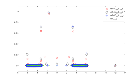
Figure 1. $\sigma(T+iQ_{51},L_{n})$ for $n=101,401,1601$ and $\sigma(T,L_{51})$.

Let $\mathcal{L}_{2n+1}={\rm span}\{e^{-inx},\dots,e^{inx}\}$. We find that $\sigma(T,\mathcal{L}_{51})$ has four eigenvalues in the interval $(-\pi,\pi)$. With $Q_{51}=E_{51}((-\pi,\pi))P_{51}$ we calculate $\sigma(T+iQ_{51},\mathcal{L}_{2n+1})$ for $n=50,200$ and $800$. The results are displayed in Figure 1, and, consistent with Theorem 3.6, suggest that $\sigma(T+iQ_{51})$ has a simple eigenvalue near $\lambda_{1}+i$.

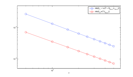
Figure 2. Convergence to $\lambda_{1}+i$ using $\sigma(T+iQ_{2n+1},L_{4n+1})$ compared to the convergence to $\lambda_{2}$ using $\sigma(T,L_{4n+1})$.

Calculating $\sigma(T+iQ_{2n+1},\mathcal{L}_{20n+1})$ with $n=4,8,12,\dots,40$ suggests that we have

(3.10) $${\rm dist}(\lambda_{1}+i,\sigma(T+iQ_{2n+1},\mathcal{L}_{20n+1}))\approx\mathcal{O}(n^{-1}).$$

The following estimate holds:

(3.11) $$\delta(\mathcal{L}(\{\lambda_{1}\}),\mathcal{L}_{2n+1})=\mathcal{O}(n^{-1/2});$$

see for example [3, Lemma 3.1]. Combining this estimate with Theorem 3.6 we obtain

(3.12) $${\rm dist}(\lambda_{1}+i,\sigma(T+iQ_{n}))=\mathcal{O}(n^{-1})$$

which is consistent with (3.10). The latter suggests that in Theorem 3.6 the convergence rate for $r_{n}$ is sharp.

For a fixed and sufficiently large $m$ we denote by $\mathcal{M}$ (respectively $\mathcal{M}^{*}$) the eigenspace associated to the simple eigenvalue of $T+iQ_{m}$ (respectively $T-iQ_{m}$) which lies in a neighbourhood of $\lambda_{1}+i$ (respectively $\lambda_{1}-i$). Then the following estimates hold:

(3.13) $$\delta(\mathcal{M},\mathcal{L}_{n})=\mathcal{O}(n^{-1/2})\quad\textrm{and}\quad\delta(\mathcal{M}^{*},\mathcal{L}_{n})=\mathcal{O}(n^{-1/2});$$

see for example [3, Lemma 3]. For the approximation of the eigenvalue $\lambda_{j}$ we calculate $\sigma(T+iQ_{2n+1},\mathcal{L}_{4n+1})$ with $n=50,100,150,\dots,500$. For comparison, we also approximate the eigenvalue $\lambda_{2}$ which lies outside the convex hull of the essential spectrum and may therefore be approximated without encountering spectral pollution. The results are displayed in Figure 2 and suggest that

(3.14) $${\rm dist}(\lambda_{1}+i,\sigma(T+iQ_{2n+1},\mathcal{L}_{4n+1}))=\mathcal{O}(n^{-1})\quad\textrm{and}$$

(3.15) $${\rm dist}(\lambda_{2},\sigma(T,\mathcal{L}_{4n+1}))=\mathcal{O}(n^{-1}).$$

The convergence in (3.14) is consistent with (3.12), (3.13) and (3.9). The convergence in (3.15) follows from (3.11) and the well-known superconvergence result for an eigenvalue lying outside the convex hull of the essential spectrum of bounded self-adjoint operator.

3.3. Unbounded Operators

We now assume that $T$ is bounded from below and unbounded from above. Let $\gamma<\min\sigma(T)$ and consider the operator $T-\gamma$. We have $[a-\gamma,b-\gamma]\cap\sigma_{\mathrm{ess}}(T-\gamma)=\varnothing$, and, in particular

(3.16) $$\left[\frac{1}{b-\gamma},\frac{1}{a-\gamma}\right]\cap\sigma_{\mathrm{ess}}((T-\gamma)^{-1})=\varnothing.$$

We shall approximate the eigenvalues $\sigma(T)\cap[a,b]$ by applying the results from the preceding sections to approximate eigenvalues of $(T-\gamma)^{-1}$ in $\sigma((T-\gamma)^{-1})\cap[(b-\gamma)^{-1},(a-\gamma)^{-1}]$.

Let $\{\mu_{1},\dots,\mu_{k}\}=[a,b]\cap\sigma(T,\mathcal{L}_{n})$ where the eigenvalues are repeated according to multiplicity. Let $\{u_{1},\dots,u_{k}\}$ be a corresponding set of orthonormal eigenvectors. We write $\hat{x}=(T-\gamma)^{\frac{1}{2}}x$ and $\hat{\mathcal{L}}_{n}=(T-\gamma)^{\frac{1}{2}}\mathcal{L}_{n}$, and note that $\hat{u}_{i}\perp\hat{u}_{j}$ for $i\neq j$ since

$$\langle\hat{u}_{i},\hat{u}_{j}\rangle=(\mathfrak{t}-\gamma)(u_{i},u_{j})=(\mu_{i}-\gamma)\langle u_{i},u_{j}\rangle=0.$$

Furthermore, we have for some $\mu_{i}\in[a,b]$ and any $y\in\mathcal{L}_{n}$

$$0=(\mathfrak{t}-\gamma)(u_{i},y)-(\mu_{i}-\gamma)\langle u_{i},y\rangle=\langle\hat{u}_{i},\hat{y}\rangle-(\mu_{i}-\gamma)\langle(T-\gamma)^{-1}\hat{u}_{i},\hat{y}\rangle,$$

so that $(\mu_{i}-\gamma)^{-1}\in\sigma((T-\gamma)^{-1},\hat{\mathcal{L}}_{n})$. Evidently, there is a one-to-one correspondence between $\sigma(T,\mathcal{L}_{n})$ and $\sigma((T-\gamma)^{-1},\hat{\mathcal{L}}_{n})$:

$$\sigma((T-\gamma)^{-1},\hat{\mathcal{L}}_{n})=\left\{\frac{1}{\lambda-\gamma}:~{}\lambda\in\sigma(T,\mathcal{L}_{n})\right\}.$$

In particular, we have

$$\sigma((T-\gamma)^{-1},\hat{\mathcal{L}}_{n})\cap\left[\frac{1}{b-\gamma},\frac{1}{a-\gamma}\right]=\left\{\frac{1}{\mu_{1}-\gamma},\dots,\frac{1}{\mu_{k}-\gamma}\right\}$$

with corresponding orthogonal eigenvectors given by $\{\hat{u}_{1},\dots,\hat{u}_{k}\}$. Denote by $Q_{n}$ the orthogonal projection onto $\operatorname{span}\{\hat{u}_{1},\dots,\hat{u}_{k}\}\subset\hat{\mathcal{L}}_{n}$. From the first paragraph in the proof of lemma 2.4 it follows that $\delta(\mathcal{L}(\Delta),\hat{\mathcal{L}}_{n})=\mathcal{O}(\delta_{\mathfrak{t}}(\mathcal{L}(\Delta),\mathcal{L}_{n}))$, then by Lemma 3.4 we have

$$Q_{n}\stackrel{{\scriptstyle s}}{{\longrightarrow}}E(\Delta)\quad\textrm{and}\quad\|(I-Q_{n})E\|=\mathcal{O}(\delta_{\mathfrak{t}}(\mathcal{L}(\Delta),\mathcal{L}_{n})).$$

Hence, a direct application of Terrorem 3.6 to the bounded self-adjoint operator $(T-\gamma)^{-1}$ and subspaces $(\hat{\mathcal{L}}_{n})$ yields the following corollary.

Corollary 3.8.

There exists sequences $(\tau_{n})$ and $(r_{n})$ of non-negative reals, with

$$0\leq\tau_{n}=\mathcal{O}(\delta_{\mathfrak{t}}(\mathcal{L}(\Delta),\mathcal{L}_{n}))\quad\textrm{and}\quad 0\leq r_{n}=\mathcal{O}(\delta_{\mathfrak{t}}(\mathcal{L}(\Delta),\mathcal{L}_{n})^{2}),$$

such that $U_{\tau_{n},r_{n}}(1/(b-\gamma),1/(a-\gamma))\backslash\mathbb{R}\subset\rho((T-\gamma)^{-1}+iQ_{n})$ for all sufficiently large $n$. Moreover, if $\Gamma_{j}$ is the circle with center $1/(\lambda_{j}-\gamma)+i$ and radius $r_{n}$, then $\Gamma_{j}\subset\rho((T-\gamma)^{-1}+iQ_{n})$ and the dimension of the spectral subspace associated to $(T-\gamma)^{-1}+iQ_{n}$ and the region enclosed by $\Gamma_{j}$ equals the dimension of $\mathcal{L}(\{\lambda_{j}\})$.

For a fixed $m$, let $u_{1},\dots,u_{k}$ be as above, and consider the eigenvalue problem: find $z\in\mathbb{C}$ for which there exists an $x\in\mathcal{L}_{n}\backslash\{0\}$ with

(3.17) $$(\mathfrak{t}-\gamma)(x,y)-iz\sum_{j=1}^{k}\frac{(\mathfrak{t}-\gamma)(x,u_{j})(\mathfrak{t}-\gamma)(u_{j},y)}{(\mathfrak{t}-\gamma)[u_{j}]}-z\langle x,y\rangle=0\quad\forall~{}y\in\mathcal{L}_{n}.$$

Evidently, this is equivalent to the eigenvalue problem: find $z\in\mathbb{C}$ for which there exists a $\hat{x}\in\hat{\mathcal{L}}_{n}\backslash\{0\}$ and

(3.18) $$\langle\hat{x},\hat{y}\rangle-iz\sum_{j=1}^{k}\frac{\langle\hat{x},\hat{u}_{j}\rangle\langle\hat{u}_{j},\hat{y}\rangle}{\|\hat{u}_{j}\|^{2}}-z\langle(T-\gamma)^{-1}\hat{x},\hat{y}\rangle=0\quad\forall~{}\hat{y}\in\hat{\mathcal{L}}_{n}.$$

The solutions to (3.18) are precisely the set $\{w^{-1}:~{}w\in\sigma((T-\gamma)^{-1}+iQ_{m},\hat{\mathcal{L}}_{n})\}$. Therefore, we may approximate the eigenvalues $\sigma((T-\gamma)^{-1})\cap[(b-\gamma)^{-1},(a-\gamma)^{-1}]$ by solving (3.17).

Example 3.9.

With $\mathcal{H}=L^{2}(0,1)\oplus L^{2}(0,1)$ we consider the block operator matrix

$$T=\left(\begin{array}[]{cc}-d^{2}/dx^{2}&-d/dx\\ d/dx&2I\end{array}\right)$$

with homogeneous Dirichlet boundary conditions in the first component. The same matrix (but with different boundary conditions) has been studied in [12]. We have $\sigma_{\mathrm{ess}}(T)=\{1\}$ (see for example [17, Example 2.4.11]) while $\sigma_{\mathrm{dis}}(T)$ consists of the simple eigenvalue $\{2\}$ with eigenvector $(0,1)^{T}$, and the two sequences of simple eigenvalues

$$\lambda_{k}^{\pm}:=\frac{2+k^{2}\pi^{2}\pm\sqrt{(k^{2}\pi^{2}+2)^{2}-4k^{2}\pi^{2}}}{2}.$$

The sequence $\lambda_{k}^{-}$ lies below, and accumulates at, the essential spectrum. While the sequence $\lambda_{k}^{+}$ lies above the eigenvalue $2$ and accumulates at $\infty$. Therefore, we have

$$\sigma_{\mathrm{ess}}(T^{-1})=\{0,1\}\quad\textrm{and}\quad\sigma_{\mathrm{dis}}(T^{-1})=\bigcup_{k=1}^{\infty}\left\{\frac{1}{\lambda_{k}^{+}}\right\}\bigcup_{k=1}^{\infty}\left\{\frac{1}{\lambda_{k}^{-}}\right\}\bigcup\left\{\frac{1}{2}\right\}.$$

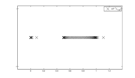
Figure 3. $\sigma(T^{-1},L_{1/49})$ displaying spectral pollution in the interval $(1/2,1)$.

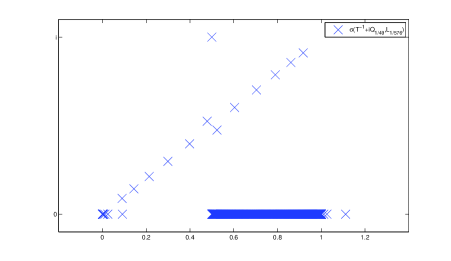
Figure 4. $\sigma(T^{-1}+iQ_{1/49},L_{1/576})$ displaying the approximation of the eigenvalue $1/2+i$.

Denote by $\mathcal{L}_{h}^{0}$ the FEM space of piecewise linear functions on a uniform mesh of size $h$ and satisfying homogeneous Dirichlet boundary conditions, and by $\mathcal{L}_{h}$ the space without boundary conditions. The subspaces $\mathcal{L}_{h}^{0}\oplus\mathcal{L}_{h}$ belong to ${\rm Dom}(\mathfrak{t})$. We define $L_{h}=T^{\frac{1}{2}}(\mathcal{L}_{h}^{0}\oplus\mathcal{L}_{h})$.

Figure 3 shows $\sigma(T^{-1},L_{1/49})$. The interval $(1/2,1)$ is filled with Galerkin eigenvalues, however, the interval $(1/2,1)$ belongs to the resolvent set of $T^{-1}$. This is an example of spectral pollution, the interval lies in the gap in the essential spectrum which is where the Galerkin method is known to be unreliable. We note that the eigenvalue $1/2$ is obscured by the spectral pollution.

Figure 4 shows $\sigma(T^{-1}+iQ_{1/49},L_{1/576})$ where $Q_{1/49}$ is the orthogonal projection associated to $\sigma(T^{-1},L_{1/49})$ and the interval $[1/4,9/10]$. Since $\sigma(T^{-1})\cap[1/4,9/10]$ consists only of the simple eigenvalue $1/2$, the set $\sigma(T^{-1}+iQ_{1/49},L_{1/576})$ has only one element with imaginary part near $1$, in fact, $1/2+i\in\sigma(T^{-1}+iQ_{1/49},L_{1/576})$ because the eigenvector associated to this eigenvalue is $\psi=(0,1)^{T}\in\mathcal{L}_{h}^{0}\oplus\mathcal{L}_{h}$, hence the eigenvalue also belongs to $L_{h}$. Therefore, our method has identified this eigenvalue, and furthermore, Figure 4 suggests that all elements $\sigma(T^{-1},L_{1/49})\cap(1/2,1)$ are points of spectral pollution.

We now turn to the approximation of the eigenvalue $1/\lambda_{1}^{+}$ which lies in the gap in the essential spectrum $(0,1)$. Figure 5 shows $\sigma(T^{-1}+iQ_{1/49},L_{1/576})$ where $Q_{1/49}$ is now the orthogonal projection associated to $\sigma(T^{-1},L_{1/49})$ and the interval $[1/20,1/5]$.

Since $\sigma(T^{-1})\cap[1/20,1/5]$ consists only of the simple eigenvalue $\{1/\lambda_{1}^{+}\}$, the set $\sigma(T^{-1}+iQ_{1/49},L_{1/576})$ has only one element with imaginary part near $1$, this is an approximation of $1/\lambda_{1}^{+}+i$. The Galerkin method does not appear to suffer from spectral pollution in the interval $(0,1/2)$. Table 1 shows the approximation of $1/\lambda_{1}^{+}$ using $\sigma(T^{-1},L_{h/2})$ and $\sigma(T^{-1}+iQ_{h},L_{h/2})$. Both converge to $1/\lambda_{1}^{+}$ with order $\mathcal{O}(h^{2})$.

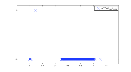
Figure 5. $\sigma(T^{-1}+iQ_{1/49},L_{1/576})$ displaying the approximation of the eigenvalue $1/\lambda_{1}^{+}+i$.

h	dist($(\lambda_{1}^{+})^{-1},\sigma(T^{-1},L_{h/2})$)	dist($(\lambda_{1}^{+})^{-1}+i,\sigma(T^{-1}+iQ_{h},L_{h/2})$)
1/9	1.852226448408184e-004	7.356900130780202e-004
1/19	4.159849994125886e-005	1.656338892411880e-004
1/39	9.875177553464454e-006	3.934129644715903e-005
1/79	2.406805040600091e-006	9.589568304944231e-006
1/159	5.941634519252004e-007	2.367430965052093e-006
1/319	1.476118197535348e-007	5.882392223781511e-007

Table 1. A comparison of the approximation of $(\lambda_{1}^{+})^{-1}$ using $\sigma(T^{-1},L_{h/2})$ and $\sigma(T^{-1}+iQ_{h},L_{h/2})$

4. Acknowledgements

The author is grateful to Marco Marletta for useful discussions and acknowledges the support of the Wales Institute of Mathematical and Computational Sciences and the Leverhulme Trust grant: RPG-167.

References

- [1] D. Boffi, F. Brezzi, L. Gastaldi, On the problem of spurious eigenvalues in the approximation of linear elliptic problems in mixed form. Math. Comp., 69 (229) (2000) 121–140.
- [2] D. Boffi, R. G. Duran, L. Gastaldi, A remark on spurious eigenvalues in a square. Appl. Math. Lett., 12 (3) (1999) 107–114.
- [3] L. Boulton, Non-variational approximation of discrete eigenvalues of self-adjoint operators. IMA J. Numer. Anal. 27 (2007) 102–121.
- [4] L. Boulton, M. Strauss, On the convergence of second-order spectra and multiplicity. Proc. R. Soc. A 467 (2011) 264–275.
- [5] F. Chatelin, Spectral Approximation of Linear Operators. Academic Press (1983).
- [6] M. Dauge & M. Suri, Numerical approximation of the spectra of non-compact operators arising in buckling problems. J. Numer. Math. (10) 2002 193- 219.
- [7] E. B. Davies, Linear Operators and their Spectra. Cambridge University Press (2007).
- [8] E. B. Davies, M. Plum, Spectral Pollution. IMA J. Numer. Anal. 24 (2004) 417–438.
- [9] T. Kato, On the upper and lower bounds of eigenvalues. J. Phys. Soc. Jpn. 4 (1949) 334- 339.
- [10] T. Kato, Perturbation theory for nullity, deficiency and other quantities of linear operators. J. Anallyse Math. 6 (1958) 261–322.
- [11] T. Kato, Perturbation Theory for Linear Operators. Springer-Verlag, Berlin, 1995.
- [12] M. Levitin, E. Shargorodsky, Spectral pollution and second order relative spectra for self-adjoint operators. IMA J. Numer. Anal. 24 (2004) 393–416.
- [13] M. Marletta, Neumann-Dirichlet maps and analysis of spectral pollution for non-self-adjoint elliptic PDEs with real essential spectrum. IMA J. Numer. Analysis 30 (2010) 917–939.
- [14] M. Marletta, R. Scheichl, Eigenvalues in Spectral Gaps of Differential Operators. J. Spectral Theory 2 (3) (2012) 293–320.
- [15] J. Rappaz, J. Sanchez Hubert, E. Sanchez Palencia & D. Vassiliev, On spectral pollution in the finite element approximation of thin elastic membrane shells. Numer. Math. 75 (1997) 473- 500.
- [16] E. Shargorodsky, Geometry of higher order relative spectra and projection methods. J. Oper. Theory, 44 (2000) 43- 62.
- [17] C. Tretter, Spectral Theory Of Block Operator Matrices And Applications. Imperial College Press (2007).
- [18] S. Zimmermann, U. Mertins, Variational bounds to eigenvalues of self-adjoint eigenvalue problems with arbitrary spectrum. Z. Anal. Anwend. 14 (1995) 327- 345.