Mass inflation inside black holes revisited

Abstract

The mass inflation phenomenon implies that black hole interiors are unstable due to a back-reaction divergence of the perturbed black hole mass function at the Cauchy horizon. Weak point in the standard mass inflation calculations is in a fallacious using of the global Cauchy horizon as a place for the maximal growth of the back-reaction perturbations instead of the local inner apparent horizon. It is derived the new spherically symmetric back-reaction solution for two counter-streaming light-like fluxes near the inner apparent horizon of the charged black hole by taking into account its separation from the Cauchy horizon. In this solution the back-reaction perturbations of the background metric are truly the largest at the inner apparent horizon, but, nevertheless, remain small. The back reaction, additionally, removes the infinite blue-shift singularity at the inner apparent horizon and at the Cauchy horizon.

1 Introduction

The mass inflation phenomenon, resulting in exponential growth of the perturbed black hole mass function at the Cauchy horizon, was considered as a fatal instability of the interior Kerr–Newman black hole solution with respect to the small perturbations (see, e. g., [1, 2, 3, 4, 5] and an example of the bounded mass inflation [6]). The specific instability of the Cauchy horizon with respect to the kink-mode perturbation was considered in the case of the Reissner–Nordström–(anti) de Sitter black hole [7]. The problem of the Cauchy horizon instability has been probed also by different numerical calculations (see, e. g., [8, 9, 10] and references therein). The mass inflation problem in the case of the rotating black holes was elaborated in [11].

The standard mass inflation calculations [1, 2, 3] are based on the using of the generalized Dray–t’ Hooft–Redmount (DTR) relation [12, 13] in the linear approximation of the Einstein equations near the perturbed inner horizon. However, the using of linear approximation to the DTR relation near horizons is a quite improper in view of the nonlinearity of the Einstein equations. This nonlinearity is especially crucial in the vicinity of the black hole horizons.

An additional weak point in the standard mass inflation calculations is in a fallacious using of the global null Cauchy horizon as a place for the maximal growth of the back-reaction perturbations instead of the local inner apparent horizon, which is separated from the Cauchy horizon. The maximal back-reaction perturbations inside the charged black hole take place (besides the central singularity) at the local inner apparent horizon and not at the separated global Cauchy horizon. This qualitative feature was missed in the previous mass inflation calculations.

It is shown below that a back-reaction of two counter-streaming light-like fluxes result in only the small corrections to the background metric near the local inner apparent horizon of the charged black hole by taking into account its separation from the Cauchy horizon. This implies the absence of the mass inflation and stability of the charged black hole interiors.

We use a (slow) quasi-stationary approximation, when both the inflowing and outflowing radial energy fluxes of light-like particles are small, $\dot{m}_{\rm in}\ll 1$ and $\dot{m}_{\rm out}\ll 1$. Respectively, the rate of black hole mass growth is also small (for more details see, e. g., [14, 15]). In finding the back-reaction in this approximation, we use the Reissner–Nordström black hole solution as a background metric and retain in equations only those perturbation terms, which are not higher, than the linear ones with respect to $\dot{m}_{\rm in}$ and $\dot{m}_{\rm out}$. In other words, we calculate the back-reaction in the linear perturbation approximation with respect to the small dimensionless energy flux parameters, $\dot{m}_{\rm in}$ and $\dot{m}_{\rm out}$.

2 Absence of mass inflation

2.1 Back-reaction metric in the $(v,r)$-frame

A general space-time metric in the spherically symmetric case can be written in the form [16, 17]:

$$ds^{2}=e^{\lambda(v,r)}dv\left[e^{\nu(v,r)+\lambda(v,r)}dv-2dr\right]-r^{2}d\Omega^{2},$$ (1)

where $d\Omega^{2}=d\theta^{2}+\sin^{2}\theta d\phi^{2}$ is a 2-sphere metric and $\lambda(v,r)$ and $\nu(v,r)$ are two arbitrary functions of two coordinates $v$ and $r$. This is a coordinate frame of the Eddington–Finkelstein type, related, in particular, with the ingoing null geodesics $v=const$. In analogy with the Schwarzschild, Reissner–Nordström and charged Vaidya metric, we use the following form for the metric function $\nu(v,r)$:

$$e^{\nu(v,r)}\equiv f\equiv 1-\frac{2m(v,r)}{r}+\frac{e^{2}}{r^{2}},$$ (2)

where $m(v,r)$ is a mass function and $e$ is an electric charge. In the special case of $\lambda(v,r)=0$, this metric is the charged Vaidya solution. Respectively, at $\lambda(v,r)=0$ and $m(v,r)=const$, this metric is the Reissner–Nordström solution.

In the back-reaction calculations, we follow very closely to [3], by using both the ingoing and outgoing Vaidya metrics as perturbations for the background Reissner–Nordström black hole metric. For the ingoing Vaidya metric in the $(v,r)$-frame we choose the mass function $m(v,r)$ in the specific form:

$$m(v,r)=m_{\rm in}(v)=\left\{\begin{array}[]{ll}\!m_{0}\left[1-\beta_{0}(v_{0}/v)^{p-1}\right]&\mbox{ at }v\geq v_{0},\\ \!m_{0}(1-\beta_{0})&\mbox{ at }v<v_{0},\end{array}\right.$$ (3)

with constants $v_{0}$, $m_{0}$, $\beta_{0}\ll 1$ and $p\geq 12$. Respectively, for the corresponding outgoing Vaidya solution in the $(u,r)$-frame we choose quite a similar expression for the mass function m(u,r):

$$m(u,r)=m_{\rm out}(u)=\left\{\begin{array}[]{ll}\!m_{0}\left[1-\beta_{1}(u_{0}/u)^{q-1}\right]&\mbox{ at }u\geq u_{0},\\ \!m_{0}(1-\beta_{1})&\mbox{ at }u<u_{0},\end{array}\right.$$ (4)

with the additional constants $u_{0}$, $\beta_{1}\ll 1$ and $q\geq 12$.

The global geometry of the Reissner–Nordström black hole, perturbed by both the ingoing and outgoing radial null fluxes, is shown in Fig. 1 by means of the Carter–Penrose diagram. The metric functions $\lambda=0$ and $\nu=0$ at both the inner and outer apparent horizons, $r=r_{\pm}(v)$ and $r=r_{\pm}(u)$, of the perturbed black hole. These local apparent horizons are the boundaries between the $R$- and $T$-regions with the different metric signatures, $(+,-,-,-)$ and $(-,+,-,-)$, respectively. The variable parts of these apparent horizons are shown by the thick curves $AB$, $FE$, $GH$ and $CD$ in Fig. 1.

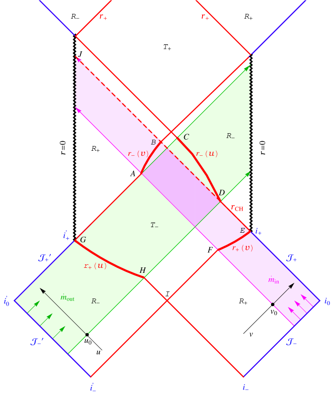
Figure 1: The Carter–Penrose diagram for the Reissner-Nordsröm black hole, perturbed by the small inflowing, $\dot{m}_{\rm in}\ll 1$, and outflowing, $\dot{m}_{\rm out}\ll 1$, radial fluxes of light-like particles, related with the corresponding ingoing and outgoing Vaidya solutions outside the black hole. Inside the black hole, i. e., at $r<r_{+}(v)$ and $r<r_{+}(u)$, there is a double filled overlapping region with two coexisting and oppositely directed fluxes. The global Cauchy horizon $r_{\rm CH}$, which is defined by the null line $v-\infty$, is shown in part by the null line $ED$ and further by the null dashed line $DBJ$. The perturbed metric deviates from the linear sum of ingoing and outgoing Vaidya metrics (due to the nonlinearity of the Einstein equations) in the space-time regions, corresponding to the all future-directed light-cones in this overlapping region. The maximal perturbation of the black hole metric, which is the most interesting for the discussed mass inflation problem. The maximal blue-shift of the inward radiation, viewed by the free-moving observer, will take place just at the part of the local inner apparent horizon $r_{-}(u)$, shown by the thick time-like curve $CD$ and not at the part of the global Cauchy horizon $r_{\rm CH}$, shown by the dashed null line $BD$.

There is only one flux, respectively, inflowing $\dot{m}_{\rm in}$ or outflowing $\dot{m}_{\rm out}$ in the filled but non-overlapping regions of the Carter–Penrose diagram in Fig. 1 for the perturbed metric. Solutions of the Einstein equations in these non-overlapping regions are the corresponding ingoing and outgoing charged Vaidya metrics. Meanwhile, both the inward and outward fluxes coexist in the overlapping region. It must be stressed, that the overlapping region exists only inside the black hole, at $r<r_{+}(v)$ and $r<r_{+}(u)$. In the overlapping region a corresponding solution of the Einstein equations deviates from the Vaidya metric. In other words, the sum of two counter-streaming Vaidya solutions is not the valid solution of the Einstein equations due to their nonlinearity. Evidently, in the regions without any fluxes (see the non filled regions in Fig. 1 the standard Reissner–Nordström metric is realized, though with the different values of the black hole mass before and after the passage of inflowing or outflowing fluxes. The metric functions $\lambda=0$ and $\nu=0$ at both the inner and outer apparent horizons, $r=r_{\pm}(v)$ and $r=r_{\pm}(u)$, of the perturbed black hole. These local apparent horizons are the boundaries between the $R$- and $T$-regions with the different metric signatures, $(+,-,-,-)$ and $(-,+,-,-)$, respectively.

A principal point is that the global Cauchy horizon $r=r_{\rm CH}$ is separated from the local inner apparent horizon $r=r_{-}(v)$ in the case of the non-stationary (perturbed) metric. This separation is clearly viewed in Fig. 1, where the global Cauchy horizon $r_{\rm CH}$ is shown in part by the null line $ED$ and further by the dashed null line $DBJ$, while the corresponding part of the inner apparent horizon $r=r_{-}(u)$ is shown by the time-like curve $CD$. The maximal perturbation of the black hole metric, which is the most interesting for the discussed mass inflation problem, and the maximal blue-shift of inward radiation, viewed by the free-moving observer, will take place just at the $r_{-}(u)$ (the time-like curve $CD$) and not at the $r_{\rm CH}$ (the null line $BD$).

The singular behavior of metric functions $\lambda$ and $\nu$ at the horizons is especially crucial when the double-null (u,v)-frame is used near horizons. In particular, it was demonstrated the ill-posedness of a double null “free” evolution scheme in numerical calculations for the Einstein equations, when constraints are imposed only at the boundaries, and all fields are propagated by means of the evolution equations [18]. This ill-posedness of the “free” evolution numerical scheme results in the artificial exponentially growing mode.

To resolve a back-reaction problem for the perturbed spherically symmetric black hole, the two sought functions $\nu$ and $\lambda$ in the general metric (1) must be calculated by using the Einstein equations with the appropriately chosen perturbations. We follow below closely to E. Poisson and W. Israel [3] by writing the Einstein equations in the form

$$G_{\alpha\beta}=8\pi(E_{\alpha\beta}+T_{\alpha\beta}),$$ (5)

where the Maxwellian contribution to the energy-momentum tensor from the black hole electric charge $e$ is

$$E^{\alpha}_{\beta}=\frac{e^{2}}{8\pi r^{4}}\,{\rm diag}(1,1,-1,-1)$$ (6)

and $T_{\alpha\beta}$ is a perturbation energy-momentum tensor.

The nonzero components of the Einstein tensor $G_{\alpha\beta}$ in the Eddington–Finkelstein frame (1) are

$$G_{0}^{0} = -e^{\nu}\left(\frac{1}{r^{2}}+\frac{\nu^{\prime}}{r}\right)+\frac{1}{r^{2}},$$ (7)

$$G_{0}^{1} = \frac{e^{\nu}}{r}\,\dot{\nu},$$ (8)

$$G_{1}^{0} = -2\frac{e^{-\lambda}}{r}\lambda^{\prime},$$ (9)

$$G_{1}^{1} = G_{0}^{0}-\frac{2\lambda^{\prime}}{r}\,e^{\nu},$$ (10)

$$G_{2}^{2} = G_{3}^{3}=-e^{\nu}\left(\lambda^{\prime\prime}+\frac{\nu^{\prime\prime}}{2}\right)-e^{-\lambda}\dot{\lambda}^{\prime}$$ (11)

$$-e^{\nu}\left(\lambda^{\prime 2}+\frac{\nu^{\prime 2}}{2}+\frac{\lambda^{\prime}+\nu^{\prime}}{r}+\frac{3}{2}\lambda^{\prime}\nu^{\prime}\right),$$

where dot  ${}^{.}\!=\partial/\partial v$, and prime  ${}^{\prime}\!=\partial/\partial r$. The corresponding Einstein equations are related by the Bianchi identity. Therefore, one of them is not independent, e. g., equation, related with the component $G_{2}^{2}$ from (11). As a background metric we consider the Reissner–Nordsröm black hole metric, which is an exact electro-vacuum solution of the Einstein equations (5) with $T_{\alpha\beta}=0$. We calculate in the following the back-reaction on the background Reissner–Nordsröm black hole metric of both the inflowing and outflowing radial fluxes of light-like particles, described by the perturbation energy-momentum tensor

$$T_{\alpha\beta}=\rho_{\rm in}l_{\alpha}l_{\beta}+\rho_{\rm out}n_{\alpha}n_{\beta}$$ (12)

with, respectively, the energy influx $\dot{m}_{\rm in}=4\pi r^{2}\rho_{\rm in}$ and outflux $\dot{m}_{\rm out}=4\pi r^{2}\rho_{\rm out}$ and the radial null vectors

$$l^{\mu} = (l^{v},l^{r},l^{\theta},l^{\phi})=(0,-1,0,0),$$ (13)

$$n^{\mu} = (n^{v},n^{r},n^{\theta},n^{\phi})=(1,\frac{1}{2}fe^{\lambda},0,0),$$ (14)

where $l^{2}=n^{2}=0$. Both the outer horizon $r_{+}$ and the inner horizon $r_{-}$ in the used quasi-stationary approximation (with a linear accuracy in $\dot{m}_{\rm in}\ll 1$ and $\dot{m}_{\rm out}\ll 1$) are solutions of the equation $f=0$ or, formally, $r_{\pm}=m(v,r)\pm\sqrt{m(v,r)^{2}-e^{2}}$ at $e^{2}\leq m(v,r)^{2}$. Note that these horizons are, respectively, the inner and outer apparent horizons for a non-stationary metric [19].

The perturbation energy-momentum tensor components in the $(v,r)$-frame (1) are

$$T^{0}_{0} = \frac{1}{2}fe^{2\lambda}\rho_{\rm out}=-T^{1}_{1},$$ (15)

$$T^{1}_{0} = e^{\lambda}(-\rho_{\rm in}+\frac{1}{4}f^{2}e^{2\lambda}\rho_{\rm out}),$$ (16)

$$T^{0}_{1} = -e^{\lambda}\rho_{\rm out},$$ (17)

$$T^{2}_{2} = T^{3}_{3}=0.$$ (18)

We calculate in the following the back-reaction solution of the Einstein equations near horizons, at $|r-r_{\pm}|/r_{\pm}\ll 1$. In the quasi-stationary approximation the both fluxes are nearly constant in the vicinity of horizons, $\dot{m}_{\rm in}=const\ll 1$ and $\dot{m}_{\rm out}=const\ll 1$, respectively. From equation (9) we get near horizons

$$e^{\lambda}\approx\left\{\begin{array}[]{ll}1&\mbox{~{}in regions without ouward flux},\\ \left(r/r_{\pm}\right)^{\dot{m}_{\rm out}}&\mbox{~{}in regions with outward flux}.\end{array}\right.$$ (19)

Respectively, from equations (7) and (10) we get

$$m^{\prime} = 4\pi r^{2}T^{0}_{0}=\frac{1}{2}\dot{m}_{\rm out}fe^{2\lambda},$$ (20)

$$\dot{m} = -4\pi r^{2}T^{1}_{0}=e^{\lambda}(\dot{m}_{\rm in}-\frac{1}{4}f^{2}e^{2\lambda}\dot{m}_{\rm out}).$$ (21)

Near horizons, where $f\ll 1$ and $\lambda\ll 1$, we have

$$m^{\prime}\approx\frac{1}{2}\,\dot{m}_{\rm out}f,\quad\dot{m}\approx\dot{m}_{\rm in}.$$ (22)

The mass function $m(v,r)$ strongly depends on the coordinate $r$ but weakly on the coordinate $v$ near $r=r_{\pm}$ in the used quasi-stationary approximation. For this reason, it is credible to adopt a factorization for the mass function near horizons (see also [14]): $m(v,r)=m(v)\mu(x)$ with the dimensionless coordinate $x=r/m_{0}$ and with the “mass” $m(v)=m_{\rm in}(v)$, where $m_{\rm in}(v)$ is from equation (3). The function $m(v)$ is weakly growing with $v$, i. e., $dm(v)/dv=\dot{m}_{\rm in}\ll 1$ and, therefore, $m(v)\approx m_{0}=const$.

To solve the first nonlinear equation in (22) near the outer and inner apparent horizons $x=x_{\pm}$, we define the black hole extreme parameter $\epsilon=\sqrt{1-e^{2}/m_{0}^{2}}$ and the new variable

$$\delta_{\pm}(x)\equiv x-x_{\pm}=x-[\mu(x)\pm\sqrt{\mu(x)^{2}-(1-\epsilon^{2})}],$$ (23)

The horizons $x=x_{\pm}$ are solutions of equation $\delta_{\pm}(x)=0$. Near horizons, at $|\delta_{\pm}|\ll 1$, we have

$$f\approx\pm 2\frac{\sqrt{\mu(x)^{2}-(1-\epsilon^{2})}}{x_{\pm}^{2}}\delta_{\pm}\approx\pm\frac{2\epsilon}{(1\pm\epsilon)^{2}}\delta_{\pm}.$$ (24)

Now the left equation in (22) is written as

$$\frac{d\mu}{dx}\approx\pm\frac{\epsilon\dot{m}_{\rm out}}{(1\pm\epsilon)^{2}}(x-x_{\pm}).$$ (25)

Solution of this equation in the non-overlapping region, where there is only influx, is $\mu(x)=1$. Evidently, this solution coincides with the corresponding ingoing Vaidya metric in the non-overlapping region in the vicinity of the null line $HD$ in Fig. 1.

Meantime, solution of the same equation (25) in the vicinity of the inner apparent horizon, at $|x-x_{-}|\ll 1$, in the overlapping region, where there are both the inward and outward fluxes, is

$$\mu(x)\approx 1-\frac{\epsilon\dot{m}_{\rm out}}{(1-\epsilon)^{2}}\frac{(x-x_{-})^{2}}{2}.$$ (26)

The resulting metric deviates from the Vaidya solution in the overlapping region near the inner apparent horizon $x=x_{-}$ (in the vicinity of the curve $HD$ in Fig. 1). The integration constant in (26) is $1$ due to continuity relation, i. e., this solution must coincide with the Vaidya solution at the inner horizon $x=x_{-}$ on the border between the overlapping and non-overlapping regions (at the point $D$ in Fig. 1).

At the same time, the solution of equation (25) near both the inner and outer apparent horizons, at $x=x_{\pm}$, in the non-overlapping regions, where there is only outward flux $\dot{m}_{\rm out}$ is the outgoing Vaidya metric:

$$\mu(x)\approx 1\pm\frac{\epsilon\dot{m}_{\rm out}}{(1\pm\epsilon)^{2}}\frac{(x-x_{\pm})^{2}}{2}.$$ (27)

This outgoing Vaidya solution, however, is presented here in the ingoing (v,r)-frame, which is non-optimal in the presence of outward flux $\dot{m}_{\rm out}$. In the outgoing (u,r)-frame the mass function $m(u,r)$ would have the vice-versa behavior.

In general, there are two variable branches of the inner apparent horizon, $r=r_{-}(v)$ and $r=r_{-}(u)$, shown by the thick curves $AB$ and $CD$ in Fig. 1. The back-reaction mass function $m(v,r)\approx m_{0}\mu(x)$ from (26) is finite at the both inner apparent horizons $AB$ and $CD$ without any indication of the mass inflation.

2.2 Back-reaction metric in the $(t,r)$-frame

An alternative approach is in using of the general spherically-symmetric metric in the Schwarzschild-like $(t,r)$-frame [17]:

$$ds^{2}=e^{\eta(t,r)}dt^{2}-e^{\sigma(t,r)}dr^{2}-r^{2}d\Omega^{2}$$ (28)

with two arbitrary functions, $\eta(t,r)$ and $\sigma(t,r)$. For application to the back-reaction problem of the accreting matter on the charged black hole, we define, additionally, two metric functions, $f_{0}(t,r)$ and $f_{1}(t,r)$ or, equivalently, two mass functions, $m_{0}(t,r)$ and $m_{1}(t,r)$:

$$e^{\eta(t,r)} \equiv f_{0}=1-\frac{2m_{0}(t,r)}{r}+\frac{e^{2}}{r^{2}},$$ (29)

$$e^{-\sigma(t,r)} \equiv f_{1}=1-\frac{2m_{1}(t,r)}{r}+\frac{e^{2}}{r^{2}}.$$ (30)

The nonzero components of the Einstein tensor $G_{\alpha\beta}$ in the $(t,r)$-frame (28) have the following form [17]:

$$G^{1}_{0} = -e^{-\sigma}\frac{\dot{\sigma}}{r},$$ (31)

$$G^{0}_{0} = -e^{-\sigma}\left(\frac{1}{r^{2}}-\frac{\sigma^{\prime}}{r}\right)+\frac{1}{r^{2}},$$ (32)

$$G^{1}_{1} = -e^{-\sigma}\left(\frac{1}{r^{2}}+\frac{\eta^{\prime}}{r}\right)+\frac{1}{r^{2}},$$ (33)

$$G^{2}_{2}=G^{3}_{3} = \frac{e^{-\eta}}{2}\left[\ddot{\sigma}+\frac{\dot{\sigma}}{2}\left(\dot{\sigma}-\dot{\eta}\right)\right]-\frac{e^{-\sigma}}{2}\left[\eta^{\prime\prime}+(\eta^{\prime}-\sigma^{\prime})\left(\frac{\eta^{\prime}}{2}+\frac{1}{x}\right)\right]\!.$$ (34)

For the inward and outward null vectors in the energy-momentum tensor (12) we choose now

$$l_{a}=(-1,-\frac{1}{\sqrt{f_{0}f_{1}}},0,0),\quad n_{a}=(1,-\frac{1}{\sqrt{f_{0}f_{1}}},0,0).$$ (35)

The corresponding perturbation energy-momentum tensor (12) is now

$$T^{0}_{0} = \frac{1}{f_{0}}(\rho_{\rm in}+\rho_{\rm out})=-T^{1}_{1},$$ (36)

$$T^{1}_{0} = \sqrt{\frac{f_{1}}{f_{0}}}(\rho_{\rm out}-\rho_{\rm in}),$$ (37)

$$T^{2}_{2} = T^{3}_{3}=0.$$ (38)

From equations (5), (31), (32) and (32) with perturbation energy-momentum tensor from (36) and (37) we get the requested back reaction equations for the mass functions $m_{0}(t,r)$ and $m_{1}(t,r)$ in the vicinity of the apparent horizons at $|r-r_{\pm}|/r_{\pm}\ll 1$, where $f_{0}\ll 1$ and $f_{1}\ll 1$:

$$\dot{m}_{1} = \frac{\partial m_{1}}{\partial t}=\sqrt{\frac{f_{1}}{f_{0}}}(\dot{m}_{\rm in}-\dot{m}_{\rm out})\ll 1,$$ (39)

$$m^{\prime}_{1} = \frac{\partial m_{1}}{\partial x}\approx\frac{\dot{m}_{\rm in}+\dot{m}_{\rm out}}{f_{0}}\approx-m^{\prime}_{0}.$$ (40)

In the quasi-stationary approximation the both mass functions, $m_{0}(t,r)$ and $m_{1}(t,r)$, strongly depend on the radial coordinate $r$, but very weakly on the time coordinate $t$. For this reason, as in the previous Section 2.1, we adopt near horizons a factorization for the mass functions: $m_{0}(t,r)=m(t)\mu_{0}(x)$ and $m_{1}(t,r)=m(t)\mu_{1}(x)$ with the dimensionless coordinate $x=r/m_{0}$ and with a weakly growing “mass” $m(t)$. We use also the variable $\delta_{\pm}$ from equation (23) to solve the nonlinear equation (40) in the vicinity of the inner and outer apparent horizons. Again, as in the Section 2.1, the outer and inner apparent horizons at $x=x_{\pm}$ are solutions of equation $\delta_{\pm}(x)=0$, where $\delta_{\pm}(x)$ is defined by equation (23). Now, near the apparent horizons, at $|x-x_{\pm}|\ll 1$, where $|\delta_{\pm}|\ll 1$, we have

$$f_{0}\approx\pm 2\frac{\sqrt{\mu_{0}(x)^{2}-(1-\epsilon^{2})}}{x_{\pm}^{2}}\delta_{\pm}\approx\pm\frac{2\epsilon}{(1\pm\epsilon)^{2}}\delta_{\pm}.$$ (41)

Respectively, equation (40) is written near the apparent horizons as

$$\mu^{\prime}_{0}=\frac{d\mu_{0}}{dx}\approx\mp\frac{(1\pm\epsilon)^{2}}{2\epsilon}\frac{\dot{m}_{\rm in}+\dot{m}_{\rm out}}{\delta_{\pm}(x)}\approx-\mu^{\prime}_{1}.$$ (42)

The resulting solutions for mass functions near the apparent horizons are

$$\mu_{0}(\delta_{\pm}) \approx \mu_{\pm}\mp\frac{(1\pm\epsilon)^{2}}{2\epsilon}\,\dot{m}\log{\left|1+\frac{2\epsilon^{2}}{(1\pm\epsilon)^{3}\dot{m}}\,\delta_{\pm}\right|},$$ (43)

$$\mu_{1}(\delta_{\pm}) \approx 2\mu_{\pm}-\mu_{0}(\delta_{\pm}).$$ (44)

Here

$$\dot{m}=\left\{\begin{array}[]{ll}\!0&\mbox{~{}in regions without fluxes},\\ \!\dot{m}_{\rm in}&\mbox{~{}in non-overlapping regions with influx},\\ \!\dot{m}_{\rm in}+\dot{m}_{\rm out}&\mbox{~{}in overlapping region},\\ \!\dot{m}_{\rm out}&\mbox{~{}in non-overlapping regions with outflux},\\ \end{array}\right.$$ (45)

and the values of mass functions at the horizons, respectively, $\mu_{+}\equiv\mu_{0}(x_{+})=\mu_{1}(x_{+})$ and $\mu_{-}\equiv\mu_{0}(x_{-})=\mu_{1}(x_{-})$ are

$$\mu_{\pm}\approx 1\mp\frac{(1\pm\epsilon)^{2}}{2\epsilon}\,\dot{m}\log{\left|\dot{m}\right|}.$$ (46)

It can be seen in Fig. 1, that all the variable parts of the horizons, i. e., the apparent horizons $r_{\pm}(u)$ and $r_{\pm}(v)$, are placed in the non-overlapping regions of the Carter–Penrose diagram, where there is only one flux, inward or outward (curves $AB$, $CD$, $EF$ and $GH$). At the same time, the constant parts of the inner and outer horizons are placed either at the borders of the non-overlapping regions with the zero fluxes (null lines $AG$ and $DE$), corresponding to the static black hole with a mass $m_{0}(1-\epsilon)$, or in the regions without any flux (null lines $FI$ and $HI$), corresponding to the static black holes with masses $m_{0}(1-\epsilon)(1-\beta_{0})$ and $m_{0}(1-\epsilon)(1-\beta_{1})$. Note, that the null line $DE$, which is a constant part of the inner apparent horizon $r_{-}(u)$ is identical to the part of Cauchy horizon $r_{\rm CH}$) of the global metric. The most interesting for us is the time-like curve $CD$ of the inner apparent horizon $r_{-}(u)$ of the perturbed black hole. The mass functions $\mu_{0}$ and $\mu_{1}$ are equal at $r=r_{-}(u)$ with a corresponding value

$$\mu_{-}\approx 1+\frac{(1-\epsilon)^{2}}{2\epsilon}\,\dot{m}_{\rm out}\log{\left|\dot{m}_{\rm out}\right|}<1.$$ (47)

according to equation (46).

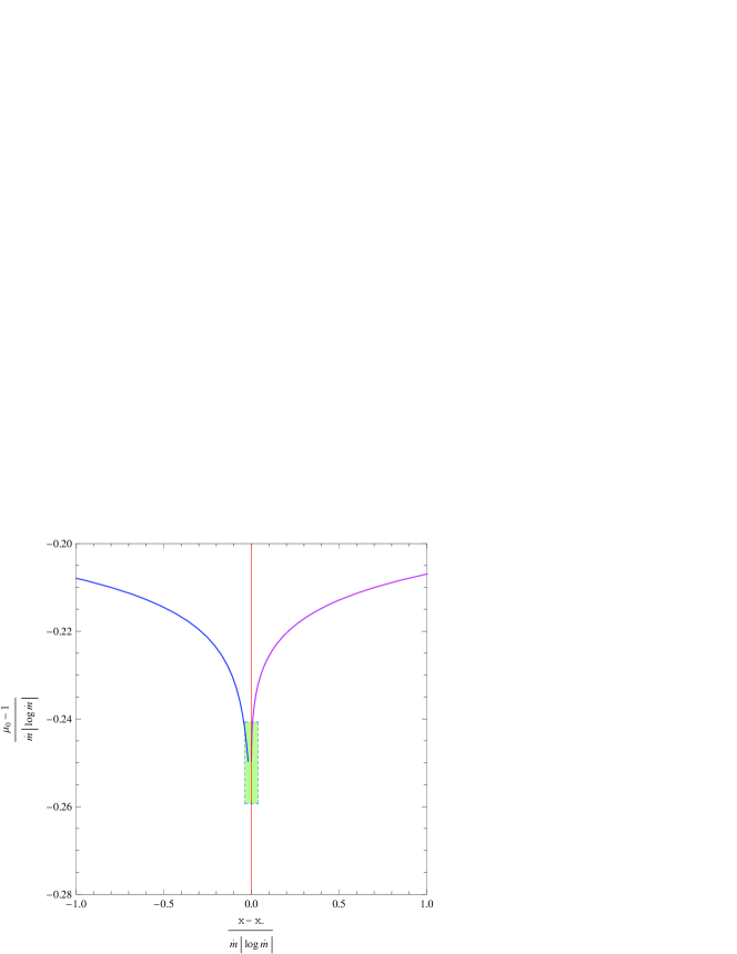
Figure 2: The mass function $\mu_{0}(x)$ from equation (43) for the black hole with the charge $e=\sqrt{3}/2$ and flux $\dot{m}=\dot{m}_{\rm out}=10^{-12}$ near the inner apparent horizon $x=x_{-}$, modified by the back-reaction. Inside the filled box the used linear perturbation approximation in $\dot{m}$ is insufficient for the exact determination of the mass function $\mu_{0}(x)$. In the used approximation, the value of the $\mu_{0}(x)$ at the $x=x_{-}$ is finite and defined by equation (47). Perturbations of the mass functions $\mu_{0}(x)$ and $\mu_{1}(x)$ remain small at the inner apparent horizon, $|\mu_{0}(x_{-})-1|=|\mu_{1}(x_{-})-1|\propto\dot{m}|\log{\dot{m}}|\ll 1$.

Solution (43) for the mass function $\mu_{0}(x)$ near horizons may be written in the form of the inverse function $x=x(\mu_{0})$, where

$$x(\mu_{0})\approx\mu_{0}\pm\!\sqrt{\mu_{0}^{2}\!-\!(1\!-\!\epsilon^{2})}\!+\!\frac{(1\pm\epsilon)^{3}\dot{m}}{2\epsilon^{2}}\left\{\!\pm\exp\left[\mp\frac{2\epsilon(\mu_{0}\!-\!\mu_{\pm})}{(1\pm\epsilon)^{2}\dot{m}}\right]\!-\!1\!\right\}\!.$$ (48)

Here, the signs $\pm$ and $\mp$ are related to the different brunches of the function $x(\mu_{0})$: the first branch for $x\leq x_{-}$ and the second one for $x\geq x_{-}$. These branches are shown in Fig. 2 for the case of $\mu_{0}(x)$ near the inner apparent horizon, corresponding to the curve $CD$ in Fig. 1, at $|x-x_{-}|\ll 1$. The first branch is at $x\leq x_{-}$ and the second one is at $x\geq x_{-}$.

With the chosen approximations, solutions (43), (44) and (48) are valid only in the narrow region $\delta_{\rm min}\equiv[(1\pm\epsilon)^{3}/\epsilon^{2}]\dot{m}<|\delta_{\pm}|\ll 1$ near the apparent horizons. In these solutions we retain only the leading perturbation terms $\sim\dot{m}|\log\dot{m}|\ll 1$ and neglect the much more smaller contributions, $\sim\dot{m}\ll 1$. The used linear perturbation approximation with respect to the small parameter $\dot{m}\ll 1$ would be insufficient for calculations of the mass functions at $|\delta_{\pm}|<|\delta_{\rm min}|$, where the quadratic perturbation terms $\propto\dot{m}^{2}$ and the higher orders ones must be taking into account. See in Fig. 2 the mass function $\mu_{0}(x)$ from equation (43) near the inner apparent horizon $x_{-}$. Note also, that divergence in (46) in the extreme limit at $\epsilon\to 0$ is related with a general instability of the perturbed extreme black hole (for some details see, e. g., [14]).

The derived solutions (43) and (44) demonstrate that the back-reaction corrections to the mass functions $m_{0}(t,r)$ and $m_{1}(t,r)$ are small near and at the inner apparent horizon of the non extreme black hole. Namely, the relative disturbance of the inner apparent horizon is small, of the order of $\dot{m}|\log{\dot{m}}|\ll 1$. Therefore, the mass inflation phenomenon is absent at least in the used quasi-stationary approximation.

3 Absence of the infinite blue-shift singularity

We calculate the blue-shift of the inward radiation viewed by a free-moving observer, traversing the non-stationary local apparent horizon $r_{-}$ or the global Cauchy horizon $r_{\rm CH}$ of the perturbed charged black hole. The new feature in this calculation, with respect to a previous similar blue-shift calculation in [3], is in taking into account, at fist, the non-stationarity of the black hole due to the presence of the influx of light-like particles and, at second, the additional perturbation, produced by the observer himself.

The appropriate place for a possible large blue-shift is a border between the $T_{-}$-region and $R_{-}$-region inside the charged black hole. In the discussed model, this border composed of the part of the inner apparent horizon $r_{-}(u)$ and the part of Cauchy horizon $r_{\rm CH}$, shown, respectively, by the time-like curve $CD$ and the null line $DE$ in Fig. 1.

Following closely to [3], we use, at first, the ingoing Vaidya solution as a background metric with a mass function $m(v)$ from equation (3). The influx of light-like particles in the ingoing Vaidya metric is described by the energy-momentum tensor $T^{\rm in}_{\alpha\beta}=\rho_{\rm in}l_{\alpha}l_{\beta}$, where $l_{\alpha}=-\partial_{\alpha}v$ and $4\pi r^{2}\rho_{\rm in}=dm_{\rm in}/dv$. The requested energy density, measured by a free-moving observer with four-velocity $u^{\alpha}$, is

$$\rho_{\rm obs}=T_{\alpha\beta}u^{\alpha}u^{\beta}=\frac{(l_{\alpha}u^{\alpha})^{2}}{4\pi r^{2}}\frac{dm_{\rm in}}{dv},$$ (49)

where $dm_{\rm in}/dv$ may be calculated, e. g., from (3). By using the four-velocity normalization $u^{\alpha}u_{\alpha}=1$, we get the trajectory equations for the free-moving observers of two dissimilar kinds (starting for simplicity somewhere inside the $T_{-}$-region in Fig. 1):

$$\dot{v}_{1,2}=f^{-1}[\dot{r}\pm[\dot{r}^{2}+f)^{1/2}],$$ (50)

where overdot denotes differentiation with respect to the observer’s proper time. Observer of the first-kind (we call him the “red-shift observer”) is traversing the border between the $T_{-}$-region and $R_{+}$-region, while the second-kind observer (we call him the “blue-shift observer”) is traversing the border between the $T_{-}$-region and $R_{-}$-region (see Fig. 1).

For the red-shift observer in the $T_{-}$-region and near the apparent horizon $r_{-}$, where $\dot{r}<0$, $0<-f\ll 1$ or $(r-r_{-})/r_{-}\ll 1$, we would have from (50) the trajectory equation

$$\dot{v}_{1}=f^{-1}[\dot{r}+[\dot{r}^{2}+f)^{1/2}]\approx-\frac{2}{\dot{r}}.$$ (51)

It is evidently seen in Fig. 1 that any red-shift observer traverses the non-stationary part of the inner apparent horizon $r_{-}$, shown by the space-like curve $AB$, at the finite values of $v$. Respectively, the value of $\dot{v}_{1}$ is finite at $r=r_{-}$ according to equation (51). In result, the red-shift observer will see the finite gravitational red-shift of the influx $\dot{m}_{\rm in}$ at the inner apparent horizon $r=r_{-}(v)$.

Meantime, for the blue-shift observer, in the same $T_{-}$-region and near the apparent or Cauchy horizons, we would have from (50) quite the different trajectory equation

$$\dot{v}_{2}=f^{-1}[\dot{r}-[\dot{r}^{2}+f)^{1/2}]\approx\frac{2\dot{r}}{f}$$ (52)

The blue-shift observer may traverse either the non-stationary part of the inner apparent horizon $r_{-}(u)$, shown by the time-like curve $CD$ in Fig. 1, or the stationary part of the inner apparent horizon, which is the part of the global Cauchy horizon, $r_{-}=r_{\rm CH}=m_{0}(1-\epsilon)=const$, shown by the null line $DE$ in Fig. 1.

The inner apparent horizon $r_{-}(u)$ is placed in the space-time beyond the null-line $v=\infty$ because $r_{-}(u)\leq r_{\rm CH}$. For this reason we need to use the $u,r$-frame for the discussed ingoing Vaidya solution to solve the trajectory equation for the blue-shift observer, traversing the inner apparent horizon $r_{-}(u)$. To circumvent this difficulty we note, that the blue-shift observer in the $(v,r)$-frame corresponds to the red-shift one in the $(u,r)$-frame. This means that a blue-shift observer will see the finite gravitational red-shift of the outflux $\dot{m}_{\rm out}$, traversing the inner apparent horizon $r=r_{-}(u)$, for the similar reasons, as the discussed earlier, the red-shift observer, traversing the inner apparent horizon $r=r_{-}(v)$.

To calculate the values of the possible blue-shift or red-shift, viewed by observers traversing the inner apparent horizons $r_{-}$, it is needed to use the geodesic equations in the perturbed Vaidya metric, which is beyond the scope of this paper. For the sake of this paper it is enough to establish that these values are finite.

Quite the contrary, the blue-shift observer traverse the Cauchy horizon $r_{\rm CH}$ at the infinite value of coordinate $v$. Therefore, $(l_{\alpha}u^{\alpha})^{2}=\dot{v}^{2}\propto f^{-2}$, is infinite at the Cauchy horizon for these observers. We integrate now equation (50) near the Cauchy horizon $r_{\rm CH}$ (i. e., in the vicinity of the null line $ED$ in Fig. 1). Differentiation of the metric function $f$ from (2) with respect to variables $v$ and $r$ with a mass function $m(v)$ for the ingoing Vaidya metric yields the trajectory equation for a free moving second kind observer in the $T_{-}$-region near the Cauchy horizon:

$$\frac{df}{dv}\approx-2\kappa_{-}\frac{dr}{dv}-\frac{2}{r_{\rm CH}}\frac{dm}{dv},$$ (53)

where

$$\kappa_{-}=\frac{\epsilon}{m_{0}(1-\epsilon)^{2}}$$ (54)

is a surface gravity at the Cauchy horizon $r_{\rm CH}=m_{0}(1-\epsilon)$. Substituting $dv/dr$ from (52) into equation (53), we obtain

$$\frac{df}{dv}+\kappa_{-}f\approx-\frac{2}{m_{0}(1-\epsilon)}\frac{dm}{dv},$$ (55)

It is crucial that a term with $dm/dv$ in (55), related with the black hole non-stationarity, was missed in previous calculations of the infinite blue-shift at the Cauchy horizon.

Solution of equation (55) with $m(v)=m_{\rm in}(v)$ from (3) is

$$f\approx-2(-1)^{p}(p-1)\frac{m_{0}\beta_{0}}{v_{0}}(k_{-}v_{0})^{p-1}e^{-k_{-}v}\,\,\Gamma(1-p,-k_{-}v),$$ (56)

where

$$\Gamma(a,x)=\int_{x}^{\infty}t^{a-1}e^{-t}dt$$ (57)

is an incomplete Gamma-function. The asymptotic form of this solution is

$$f\approx-2\beta_{0}\frac{p-1}{1-\epsilon}\left(\frac{v_{0}}{v}\right)^{p}\propto v^{-p}\quad\mbox{at }\quad v\gg v_{0}.$$ (58)

We neglect in this expression the terms of the order of $1/v^{p+1}$ and higher. In result, $\rho_{\rm obs}\propto v^{p}$ at $v\gg v_{0}$, indicating the power-law blue-shift divergence at the Cauchy horizon at $v\to\infty$. E. Poisson and W. Israel obtained a much more stronger exponential divergence for $\rho_{\rm obs}$ (see, e. g., Eqs. (B7) and (B8) in [3]) by neglecting the black hole non-stationarity, i. e., by putting $dm_{\rm in}/dv=0$ in equation (55).

The derived blue-shift at the Cauchy horizon $r=r_{\rm CH}$ is infinite for quite a formal reason: it was considered the static black hole metric with $r_{\rm CH}=const$ with the ignorance of the inevitable perturbation of the black hole metric, produced by the moving observer. This perturbation, even if extremely small, will separate the local inner apparent horizon $r_{-}(u)$ from the global Cauchy horizon. Physically, this metric perturbation from the free moving observer may be qualitatively modeled by the discussed outflux $\dot{m}_{\rm out}\ll 1$. In result, the blue-shift observer will traverse the local inner apparent horizon $r_{-}(u)$, viewing only the finite blue-shift of the influx. Note that the blue-shift observer will not see any considerable blue-shift of ingoing radiation $\dot{m}_{\rm in}$ at the dashed part of the Cauchy horizon $r=r_{\rm CH}$ (null line $BD$ in Fig. 1).

4 Conclusion

Solution of the perturbation back reaction problem for the non extreme Reissner-Nordström black hole reveals no indication of the mass inflation by taking into account the separation of the inner apparent horizon from the Cauchy horizon in the (slow) quasi-stationary accretion approximation. This separation was missed in the previous calculations of the mass inflation phenomenon.

The relative back-reaction corrections to the perturbed metric in the (v,r)-frame and (t,r)-frame at the finite distance from both the inner and outer apparent horizons, $|r-r_{\pm}|/r_{\pm}\sim 1$, appear to be of the order of small accretion rate, $\dot{m}\ll 1$, which is a small dimensionless energy flux parameter. At the same tine, near and at the apparent horizons, at $|r-r_{\pm}|/r_{\pm}\ll 1$, the relative back-reaction corrections to the black hole metric are the largest, but still remain the small, of the order of $\dot{m}\log{\dot{m}}\ll 1$. This means the absence of mass inflation phenomenon inside the charged black hole. Additionally, it shown that a back reaction removes the infinite blue-shift singularity at the inner apparent horizon.

There are a lot of limitations to the validity of the derived back-reaction corrections. The most vulnerable approximation is the slow accretion rate. It must be stressed also that semi-classical effects may influence the behavior of matter in the vicinity of the Cauchy horizon. Note also that the left patch of the Carter-Penrose diagram of the used eternal black hole geometry is absent in the general gravitational collapse. A further clarification of the mass inflation problem is required beyond the quasi-stationary limit, e. g., by using the detailed numerical calculations with the large accretion rate.

References

References

- [1] Poisson E and Israel W 1989 Phys. Rev. Lett.63 1663
- [2] Poisson E and Israel W 1989 Phys. Lett.B 233 74
- [3] Poisson E and Israel W 1990 Phys. Rev.D 41 1796
- [4] Hamilton A J S and Avelino P P 2010 Phys. Rep. 495 1 (arXiv:0811.1926 [gr-qc])
- [5] Hwang Dong-il, Lee Bum-Hoon and Yeom Dong-han 2011 JCAP 12 006 (arXiv:1110.0928 [gr-qc])
- [6] Brady P R, Nunez D and Sinha S 1993 Phys. Rev.D 47 4239 (arXiv:gr-qc/9211026)
- [7] Maeda H, Torii T and Harada T 2005 Phys. Rev.D 71 064015 (arXiv:gr-qc/0501042)
- [8] Hod S and Piran T 1998 Phys. Rev. Lett.81 1554 (arXiv:gr-qc/9803004)
- [9] Hod S and Piran T 1998 Gen. Rel. Grav. 30 1555 (arXiv:gr-qc/9902008)
- [10] Hong S E, Hwang D, Stewart E D and Yeom D 2010 Class. Quantum Grav.27 045014 (arXiv:0808.1709 [gr-qc])
- [11] Ori A 1992 Phys. Rev. Lett.68 2117
- [12] Redmount I H 1985 Prog. Ther. Phys. 73 1401
- [13] Dray T and ’t Hooft 1985 Comm. Math. Phys. 99 613
- [14] Dokuchaev V I and Eroshenko Yu N 2011 Phys. Rev.D 84 124022 (arXiv:1107.3322 [gr-qc])
- [15] Babichev E, Dokuchaev V and Eroshenko Yu 2012 Class. Quantum Grav.29 115002 (arXiv:1202.2836 [gr-qc])
- [16] Bondi H 1964 Proc. R. Soc.(London) A 281 39
- [17] Landau L D and Lifshitz E M 1975 The classical theory of fields (Oxford: Pergamon Press)
- [18] Gundlach C and Pullin J 1997 Class. Quantum Grav.14 991 (arXiv:gr-qc/9606022)
- [19] Booth I and Martin J 2010 Phys. Rev.D 82, 124046 (arXiv:1007.1642 [gr-qc])