Quasistationarity in a long-range interacting model of particles moving on a sphere

Abstract

We consider a long-range interacting system of $N$ particles moving on a spherical surface under an attractive Heisenberg-like interaction of infinite range, and evolving under deterministic Hamilton dynamics. The system may also be viewed as one of globally coupled Heisenberg spins. In equilibrium, the system has a continuous phase transition from a low-energy magnetized phase, in which the particles are clustered on the spherical surface, to a high-energy homogeneous phase. The dynamical behavior of the model is studied analytically by analyzing the Vlasov equation for the evolution of the single-particle distribution, and numerically by direct simulations. The model is found to exhibit long lived non-magnetized quasistationary states (QSSs) which in the thermodynamic limit are dynamically stable within an energy range where the equilibrium state is magnetized. For finite $N$, these states relax to equilibrium over a time that increases algebraically with $N$. In the dynamically unstable regime, non-magnetized states relax fast to equilibrium over a time that scales as $\log N$. These features are retained in presence of a global anisotropy in the magnetization.

I Introduction

Long-range interacting systems abound in nature review1 ; review2 ; review3 ; review4 ; review5 ; review6 . In these systems, the interparticle potential in $d$ dimensions decays at large separation, $r$, as $1/r^{\alpha}$, with $0\leq\alpha\leq d$. Some common examples are self-gravitating systems Jeans:1919 ; Paddy:1990 , non-neutral plasmas Nicholson:1992 , two-dimensional geophysical vortices Chavanis:2002 , dipolar ferroelectrics and ferromagnets Landau:1960 , and many others. An important feature resulting from long-range interactions is the property of non-additivity, whereby thermodynamic quantities scale superlinearly with the system size. This results in equilibrium properties which are generically not observed in short-range systems, e.g., a negative microcanonical specific heat Lynden-Bell:1968 ; Thirring:1970 , inequivalence of statistical ensembles Barre:2001 ; Mukamel:2005 ; see Bouchet:2005 for a discussion on classification of ensemble inequivalence in long-range systems.

Non-additivity also has important consequences on the dynamical properties, manifesting in broken ergodicity Mukamel:2005 ; Borgonovi:2004 ; Borgonovi:2006 ; Bouchet:2008 and intriguingly slow relaxation towards Boltzmann-Gibbs (BG) equilibrium Mukamel:2005 ; Chavanis:2002 ; Ruffo:1995 ; Yamaguchi:2004 ; Campa:2007 ; Joyce:2010 . One of the first demonstrations of such slow relaxation has been in the context of globular clusters for which dynamical evolution from a non-steady initial to a quasistationary state has been shown to be as long as 20 to 30 million years Henon:1964 . A paradigmatic toy model that has been employed over the years for much theoretical and numerical analysis of slow relaxation in long-range interacting systems is the so-called Hamiltonian mean-field (HMF) model. The model comprises globally coupled particles moving on a unit circle and interacting via an attractive $XY$-like interaction. The system evolves under deterministic Hamilton dynamics. In this model, it has been found that for a wide class of initial states, which have been termed quasistationary states (QSSs), the relaxation time to equilibrium diverges with the system size Ruffo:1995 . Moreover, for some energies, generic initial states relax on a fast timescale of order one to such long-lived QSSs Yamaguchi:2004 ; Jain:2007 . As a consequence, such systems in the thermodynamic limit never attain the BG equilibrium but remains trapped in the QSSs. Over the years, there have been several theoretical studies aimed at explaining the observed features of QSSs in the HMF model Antoniazzi:2007 ; Levin:2013 ; Ettoumi:2013 . Besides this model, QSSs have been observed in many physical systems including single-pass high-gain free electron laser Barre:2004 and two-dimensional electron plasma trapped in magnetic field Kawahara:2006 .

In order to probe the ubiquity of quasistationary behavior, various extensions of the HMF model have been introduced and analyzed over the years. For example, it has been demonstrated that while anisotropic versions of the HMF model do exhibit QSSs Jain:2007 , introducing stochastic processes into the dynamics tends to destroy QSSs leading to non-divergent relaxation times Baldovin:2006 ; Baldovin:20061 ; Baldovin:2009 ; Gupta:2010 ; Gupta:20101 ; Chavanis:2011 . A very interesting generalization of the model to that of particles moving on the surface of a sphere rather than on a circle has recently been introduced Nobre:2003 ; Nobre:2004 . Here, the model is defined on a larger phase space with each particle characterized by two positional degrees of freedom rather than one as is the case for the HMF model. In this model, the particles interact via an attractive Heisenberg-like interaction of infinite range. The model may also be viewed as one of globally coupled Heisenberg spins. The dynamics of the system follows deterministic Hamilton equations of motion. In equilibrium, the system exhibits a continuous phase transition from a low-energy magnetized phase in which the particles are clustered on the spherical surface, across critical threshold energy $\epsilon_{c}$, to a high-energy homogeneous phase. Numerical studies of the model have shown that it exhibits a number of quasistationary states, with relaxation times which diverge with the system size Nobre:2003 ; Nobre:2004 . It would be interesting to study analytically the relaxation processes in this higher dimensional model and trace the origin of its slow dynamics.

In this paper, we study analytically the relaxation dynamics of the model of particles moving on a spherical surface, within the framework of the Vlasov equation. In the limit $N\to\infty$, this equation describes the time evolution of the single-particle phase space distribution. We show that there is an energy range $\epsilon^{\star}<\epsilon<\epsilon_{c}$ where the BG equilibrium state is magnetized, in which non-magnetized quasistationary states exist. This is manifested by the fact that these states are linearly stable stationary solutions of the Vlasov equation. For finite $N$, however, such states relax to the equilibrium magnetized state over a time that scales algebraically with $N$. For energies below $\epsilon^{\star}$, non-magnetized states, though stationary, are linearly unstable under the Vlasov dynamics. Consequently, the system exhibits a fast relaxation out of such initial states. These features remain unaltered on adding a term to the Hamiltonian accounting for a global anisotropy in the magnetization.

The paper is organized as follows. In section II, we describe the model of study, and analyze the Vlasov equation to examine the relaxation dynamics. In particular, we show the existence of non-magnetized QSSs in a specific energy range within the thermodynamically stable magnetized phase. In section III, we treat the case of an additional global anisotropy in the Hamiltonian, and show similarities in the relaxation dynamics when compared with the bare model. Finally, we draw our conclusions in section IV.

II Isotropic Heisenberg mean-field model

Consider a system of $N$ interacting particles moving on the surface of a unit sphere. The generalized coordinates of the $i$-th particle are the spherical polar angles $\theta_{i}\in[0,\pi]$ and $\phi_{i}\in[0,2\pi]$, while the corresponding generalized momenta are $p_{\theta_{i}}$ and $p_{\phi_{i}}$. The Hamiltonian of the system is given by

$$H=\frac{1}{2}\sum_{i=1}^{N}\Big{(}p_{\theta_{i}}^{2}+\frac{p_{\phi_{i}}^{2}}{\sin^{2}\theta_{i}}\Big{)}+\frac{1}{2N}\sum_{i,j=1}^{N}\Big{[}1-{\bf S}_{i}\cdot{\bf S}_{j}\Big{]}.$$ (1)

Here, ${\bf S}_{i}$ is the vector pointing from the center to the position of the $i$-th particle on the sphere, and has the Cartesian components $(S_{ix},S_{iy},S_{iz})=(\sin\theta_{i}\cos\phi_{i},\sin\theta_{i}\sin\phi_{i},\cos\theta_{i})$. The term involving the double sum in Eq. (1) describes the mean-field interaction between the particles. The prefactor $1/N$ in the double sum makes the energy extensive, in accordance with the Kac prescription Kac:1963 . Nevertheless, the system is non-additive. This means that dividing the system into macroscopic subsystems and summing over their thermodynamic variables such as energy or entropy does not yield the corresponding variables of the whole system. Regarding the vector ${\bf S}_{i}$ as the classical Heisenberg spin vector of unit length, the interaction term has a form similar to that in a mean-field Heisenberg model of magnetism. However, unlike the latter case, the Poisson bracket between the components of ${\bf S}_{i}$’s in our model is zero.

The interaction term in (1) tries to cluster the particles, and is in competition with the kinetic energy term (the term involving $p_{\theta_{i}}$ and $p_{\phi_{i}}$) which has the opposite effect. The degree of clustering is conveniently measured by the “magnetization” vector ${\bf m}=(m_{x},m_{y},m_{z})=(1/N)\sum_{i=1}^{N}{\bf S}_{i}$. In the BG equilibrium state, the system exhibits a continuous phase transition at the critical energy density $\epsilon_{c}=5/6$, between a low-energy clustered (“magnetized”) phase in which the particles are close together on the sphere, and a high-energy homogeneous (“non-magnetized”) phase in which the particles are uniformly distributed on the sphere Nobre:2003 ; Nobre:2004 . As a function of the energy, the magnitude of ${\bf m}$, given by $m=\sqrt{m_{x}^{2}+m_{y}^{2}+m_{z}^{2}}$, decreases continuously from unity at zero energy density to zero at $\epsilon_{c}$, and remains zero at higher energies.

The time evolution of the system (1) follows the Hamilton equations of motion, which for the $i$-th particle are given by

$$\frac{d\theta_{i}}{dt}=p_{\theta_{i}},$$ (2)

$$\frac{d\phi_{i}}{dt}=\frac{p_{\phi_{i}}}{\sin^{2}\theta_{i}},$$ (3)

$$\frac{dp_{\theta_{i}}}{dt}=\frac{p^{2}_{\phi_{i}}\cos\theta_{i}}{\sin^{3}\theta_{i}}$$

$$+m_{x}\cos\theta_{i}\cos\phi_{i}+m_{y}\cos\theta_{i}\sin\phi_{i}-m_{z}\sin\theta_{i},$$ (4)

$$\frac{dp_{\phi_{i}}}{dt}=-m_{x}\sin\theta_{i}\sin\phi_{i}+m_{y}\sin\theta_{i}\cos\phi_{i}.$$ (5)

The dynamics conserves the total energy and the total momentum.

Here, we study how does the system starting far from equilibrium and evolving under the dynamics, Eqs. (2)-(5), relax to the equilibrium state. To this end, we now derive the Vlasov equation for the evolution of the phase space density. It is known that for a mean-field system such as ours, this equation faithfully describes the $N$-particle dynamics for finite time in the limit $N\to\infty$ Braun:1977 . In our case, we conveniently study the dynamics by analyzing the motion of a single particle in the four-dimensional phase space of its canonical coordinates $(\theta,\phi,p_{\theta},p_{\phi})$, due to the mean-field produced by its interaction with all the other particles. Let $f(\theta,\phi,p_{\theta},p_{\phi},t)$ be the probability density in this single-particle phase space, such that $f(\theta,\phi,p_{\theta},p_{\phi},t)d\theta d\phi dp_{\theta}dp_{\phi}$ gives the probability at time $t$ to find the particle with its generalized coordinates in $(\theta,\theta+d\theta)$ and $(\phi,\phi+d\phi)$, and the corresponding momenta in $(p_{\theta},p_{\theta}+dp_{\theta})$ and $(p_{\phi},p_{\phi}+dp_{\phi})$. Noting that the “velocity field” $(d\theta/dt,d\phi/dt,dp_{\theta}/dt,dp_{\phi}/dt)$ in the phase space is divergence-free, conservation of probability implies that the total time derivative of $f$ vanishes:

$$\frac{df}{dt}=\frac{\partial f}{\partial t}+\frac{d\theta}{dt}\frac{\partial f}{\partial\theta}+\frac{d\phi}{dt}\frac{\partial f}{\partial\phi}+\frac{dp_{\theta}}{dt}\frac{\partial f}{\partial p_{\theta}}+\frac{dp_{\phi}}{dt}\frac{\partial f}{\partial p_{\phi}}=0.$$ (6)

Using Eqs. (2)-(5) in the above equation, we get the Vlasov equation for time evolution of $f(\theta,\phi,p_{\theta},p_{\phi},t)$ as

$$\frac{\partial f}{\partial t}+p_{\theta}\frac{\partial f}{\partial\theta}+\frac{p_{\phi}}{\sin^{2}\theta}\frac{\partial f}{\partial\phi}+\Big{(}\frac{p^{2}_{\phi}\cos\theta}{\sin^{3}\theta}+m_{x}\cos\theta\cos\phi+m_{y}\cos\theta\sin\phi-m_{z}\sin\theta\Big{)}\frac{\partial f}{\partial p_{\theta}}$$

$$+(-m_{x}\sin\theta\sin\phi+m_{y}\sin\theta\cos\phi)\frac{\partial f}{\partial p_{\phi}}=0;$$ (7)

$$(m_{x},m_{y},m_{z})=\int d\theta d\phi dp_{\theta}dp_{\phi}~{}(\sin\theta\cos\phi,\sin\theta\sin\phi,\cos\theta)f.$$ (8)

Now, it is easily verified that any distribution $f^{(0)}(\theta,\phi,p_{\theta},p_{\phi})=\Phi(e(\theta,\phi,p_{\theta},p_{\phi}))$, with arbitrary function $\Phi$, and $e$ being the single-particle energy,

$$e(\theta,\phi,p_{\theta},p_{\phi})=\frac{1}{2}\Big{(}p_{\theta}^{2}+\frac{p_{\phi}^{2}}{\sin^{2}\theta}\Big{)}$$

$$-m_{x}\sin\theta\cos\phi-m_{y}\sin\theta\sin\phi-m_{z}\cos\theta,$$ (9)

is stationary under the Vlasov dynamics (7). The magnetization components $m_{x},m_{y},m_{z}$ are determined self-consistently. As a specific example, consider a stationary state which is non-magnetized, that is, $m_{x}=m_{y}=m_{z}=0$, and $f^{(0)}(\theta,\phi,p_{\theta},p_{\phi})$ is given by

$$f^{(0)}(\theta,\phi,p_{\theta},p_{\phi})=\left\{\begin{array}[]{ll}&\frac{1}{2\pi}\frac{1}{\pi}A\mbox{~{}~{}if~{}}\frac{1}{2}\Big{(}p_{\theta}^{2}+\frac{p_{\phi}^{2}}{\sin^{2}\theta}\Big{)}<E;\\ &\theta\in[0,\pi],\phi\in[0,2\pi],A,E\geq 0,\\ &0,\mbox{~{}~{}~{}~{}~{}~{}~{}~{}otherwise}.\end{array}\right.\\$$ (10)

The state (10) is a straightforward generalization of the well-studied water-bag initial condition for the HMF model review3 ; Note:Tsallis . The parameters $A$ and $E$ are related through the normalization condition,

$$\int_{0}^{\pi}d\theta\int_{0}^{2\pi}d\phi\int_{\Omega}dp_{\theta}dp_{\phi}f^{(0)}=1,$$ (11)

where the integration over $p_{\theta}$ and $p_{\phi}$ is over the domain $\Omega$ defined as

$$\Omega=\Theta\Big{(}2E-p_{\theta}^{2}-\frac{p_{\phi}^{2}}{\sin^{2}\theta}\Big{)},$$ (12)

with $\Theta(x)$ denoting the unit step function. Performing the integration in Eq. (11), we get

$$E=\frac{1}{4A}.$$ (13)

The conserved energy density $\epsilon$, given by

$$\epsilon = \frac{1}{2}+\int_{0}^{\pi}d\theta\int_{0}^{2\pi}d\phi\int_{\Omega}dp_{\theta}dp_{\phi}\frac{1}{2}\Big{(}p_{\theta}^{2}+\frac{p_{\phi}^{2}}{\sin^{2}\theta}\Big{)}f^{(0)},$$

is related to the parameter $E$ as

$$\epsilon=\frac{1}{2}+\frac{E}{2}.$$ (15)

We now examine the stability of the stationary state (10) under the dynamics (7). In particular, we will study linear stability. To this end, consider small perturbation around the state $f^{(0)}$, so that the corresponding state may be expanded as

$$f(\theta,\phi,p_{\theta},p_{\phi},t)=f^{(0)}+\delta f(\theta,\phi,p_{\theta},p_{\phi},t);~{}~{}\delta f\ll 1.$$ (16)

Since both $f$ and $f^{(0)}$ are normalized, we have

$$\int d\theta d\phi dp_{\theta}dp_{\phi}\delta f(\theta,\phi,p_{\theta},p_{\phi},t)=0.$$ (17)

Using Eq. (16) in Eq. (7), and keeping terms to linear order in $\delta f$, we get

$$\frac{\partial\delta f}{\partial t}+p_{\theta}\frac{\partial\delta f}{\partial\theta}+\frac{p_{\phi}}{\sin^{2}\theta}\frac{\partial\delta f}{\partial\phi}+\frac{p^{2}_{\phi}\cos\theta}{\sin^{3}\theta}\frac{\partial\delta f}{\partial p_{\theta}}$$

$$+(\widetilde{m}_{x}\cos\theta\cos\phi+\widetilde{m}_{y}\cos\theta\sin\phi-\widetilde{m}_{z}\sin\theta)\frac{\partial f^{(0)}}{\partial p_{\theta}}$$

$$+(-\widetilde{m}_{x}\sin\theta\sin\phi+\widetilde{m}_{y}\sin\theta\cos\phi)\frac{\partial f^{(0)}}{\partial p_{\phi}}=0;$$ (18)

$$(\widetilde{m}_{x},\widetilde{m}_{y},\widetilde{m}_{z})$$

$$=\int d\theta d\phi dp_{\theta}dp_{\phi}~{}(\sin\theta\cos\phi,\sin\theta\sin\phi,\cos\theta)\delta f.$$ (19)

The linearized dynamics at long times is expected to be dominated by the mode corresponding to the largest eigenfrequency $\omega$ of the linearized equation (18), so that we may write

$$\delta f(\theta,\phi,p_{\theta},p_{\phi},t)=\widetilde{\delta f}(\theta,\phi,p_{\theta},p_{\phi},\omega)e^{i\omega t}.$$ (20)

When the state (10) is linearly unstable, the system gets magnetized, which due to the complete isotropy of the Hamiltonian (1) may be taken to be along the $z$ direction without any loss of generality. This implies (and is implied by) a form of perturbation which is uniform in $\phi$:

$$\widetilde{\delta f}(\theta,\phi,p_{\theta},p_{\phi},\omega)=\frac{1}{2\pi}g(\theta,p_{\theta},p_{\phi},\omega).$$ (21)

In this case, it follows from Eq. (5) that for all $i$,

$$p_{\phi_{i}}={\rm constant},$$ (22)

equal to its initial value, so that

$$\int d\theta dp_{\theta}g(\theta,p_{\theta},p_{\phi},\omega)=0.$$ (23)

Using the above arguments and Eq. (18), it follows that corresponding to the neutral mode $\omega=0$, the quantity $g_{0}=g(\theta,p_{\theta},p_{\phi},0)$ satisfies

$$p_{\theta}\frac{\partial g_{0}}{\partial\theta}+\frac{p^{2}_{\phi}\cos\theta}{\sin^{3}\theta}\frac{\partial g_{0}}{\partial p_{\theta}}$$

$$-\frac{A}{2\pi^{2}}\Big{[}\delta(p_{\theta}+p_{0}(\theta,p_{\phi}))-\delta(p_{\theta}-p_{0}(\theta,p_{\phi}))\Big{]}\widetilde{m}_{z,0}\sin\theta=0,$$

(24)

where $\delta$ is the Dirac Delta function, while

$$\widetilde{m}_{z,0}=2\pi\int_{0}^{\pi}d\theta\cos\theta\int_{\Omega}dp_{\theta}dp_{\phi}g_{0},$$ (25)

and

$$p_{0}(\theta,p_{\phi})=\sqrt{2E-p_{\phi}^{2}/\sin^{2}\theta}.$$ (26)

In arriving at Eq. (24), we have used Eq. (10) to obtain

$$\frac{\partial f^{(0)}}{\partial p_{\theta}}=\frac{A}{2\pi^{2}}\Big{[}\delta(p_{\theta}+p_{0}(\theta,p_{\phi}))-\delta(p_{\theta}-p_{0}(\theta,p_{\phi}))\Big{]}.$$ (27)

From Eq. (24), we see that $g_{0}$ has the property

$$g_{0}(\theta,p_{\theta},p_{\phi})=-g_{0}(\pi-\theta,p_{\theta},p_{\phi}).$$ (28)

We now solve Eq. (24) for $g_{0}$. To proceed, consider a solution of the form

$$g_{0}(\theta,p_{\theta},p_{\phi}) = \Big{[}a(\theta,p_{\phi})\delta(p_{\theta}+p_{0}(\theta,p_{\phi}))$$ (29)

$$+b(\theta,p_{\phi})\delta(p_{\theta}-p_{0}(\theta,p_{\phi}))\Big{]}.$$

Equation (23) then implies that

$$\int d\theta\Big{(}a(\theta,p_{\phi})+b(\theta,p_{\phi})\Big{)}=0.$$ (30)

Also, Eq. (28) implies that

$$a(\pi/2,p_{\phi})=b(\pi/2,p_{\phi})=0.$$ (31)

Substituting Eq. (29) into Eq. (24) gives

$$\frac{p^{2}_{\phi}\cos\theta}{\sin^{3}\theta}a\Big{(}1+\frac{p_{\theta}}{p_{0}(\theta,p_{\phi})}\Big{)}\delta^{\prime}(p_{\theta}+p_{0}(\theta,p_{\phi}))$$

$$-\Big{(}p_{0}(\theta,p_{\phi})\frac{\partial a}{\partial\theta}+\frac{A}{2\pi^{2}}\widetilde{m}_{z,0}\sin\theta\Big{)}\delta(p_{\theta}+p_{0}(\theta,p_{\phi}))=0,$$

(32)

$$\frac{p^{2}_{\phi}\cos\theta}{\sin^{3}\theta}b\Big{(}1-\frac{p_{\theta}}{p_{0}(\theta,p_{\phi})}\Big{)}\delta^{\prime}(p_{\theta}-p_{0}(\theta,p_{\phi}))$$

$$+\Big{(}p_{0}(\theta,p_{\phi})\frac{\partial b}{\partial\theta}+\frac{A}{2\pi^{2}}\widetilde{m}_{z,0}\sin\theta\Big{)}\delta(p_{\theta}-p_{0}(\theta,p_{\phi}))=0.$$

(33)

Using $x\delta^{\prime}(x)=-\delta(x)$, the above equations give

$$-\Big{(}\frac{d(ap_{0}(\theta,p_{\phi}))}{d\theta}+\frac{A}{2\pi^{2}}\widetilde{m}_{z,0}\sin\theta\Big{)}\delta(p_{\theta}+p_{0}(\theta,p_{\phi}))=0,$$

(34)

$$\Big{(}\frac{d(bp_{0}(\theta,p_{\phi}))}{d\theta}+\frac{A}{2\pi^{2}}\widetilde{m}_{z,0}\sin\theta\Big{)}\delta(p_{\theta}-p_{0}(\theta,p_{\phi}))=0.$$

(35)

We thus have

$$\frac{da(\theta,p_{\phi})p_{0}(\theta,p_{\phi})}{d\theta}=\frac{db(\theta,p_{\phi})p_{0}(\theta,p_{\phi})}{d\theta}=-\frac{A\widetilde{m}_{z,0}\sin\theta}{2\pi^{2}}.$$

(36)

Integrating between $\theta^{\prime}=\pi/2$ and $\theta^{\prime}=\theta$, and using Eq. (31), we get

$$a(\theta,p_{\phi})=b(\theta,p_{\phi})=\frac{A\widetilde{m}_{z,0}\cos\theta}{2\pi^{2}p_{0}(\theta,p_{\phi})}.$$ (37)

We therefore have from Eq. (29) the solution of the linearized Vlasov equation (24) as

$$g_{0}(\theta,p_{\theta},p_{\phi})=\frac{A\widetilde{m}_{z,0}\cos\theta}{2\pi^{2}p_{0}(\theta,p_{\phi})}$$

$$\times\Big{[}\delta(p_{\theta}+p_{0}(\theta,p_{\phi}))+\delta(p_{\theta}-p_{0}(\theta,p_{\phi}))\Big{]}$$

$$=\frac{A\widetilde{m}_{z,0}\cos\theta}{\pi^{2}}\delta^{2}(2E-p_{\theta}^{2}-p_{\phi}^{2}/\sin^{2}\theta),$$ (38)

which is invariant under rotation about the $z$-axis, as it should be.

Equations (25) and (38) give a self-consistent equation for $\widetilde{m}_{z,0}$, as follows:

$$\widetilde{m}_{z,0}=2\pi\int_{0}^{\pi}d\theta\cos\theta\int_{-\sqrt{2E}\sin\theta}^{\sqrt{2E}\sin\theta}dp_{\phi}\int_{-\sqrt{2E-p^{2}_{\phi}/\sin^{2}\theta}}^{\sqrt{2E-p^{2}_{\phi}/\sin^{2}\theta}}dp_{\theta}g_{0}(\theta,p_{\theta},p_{\phi})$$

$$=\frac{A\widetilde{m}_{z,0}}{\pi^{2}}2\pi\int_{0}^{\pi}d\theta\cos^{2}\theta\int_{-\sqrt{2E}\sin\theta}^{\sqrt{2E}\sin\theta}dp_{\phi}\frac{dp_{\phi}}{\sqrt{2E-p_{\phi}^{2}/\sin^{2}\theta}}$$

$$=\frac{4A\widetilde{m}_{z,0}}{3}.$$ (39)

We therefore have the desired self-consistent equation for $\widetilde{m}_{z,0}$:

$$\widetilde{m}_{z,0}\Big{[}1-\frac{4A}{3}\Big{]}=0.$$ (40)

Then, since $\widetilde{m}_{z,0}\neq 0$, the above equation is satisfied with $A=A^{\star}$, where $A^{*}=3/4$. Correspondingly, on using Eqs. (13) and (15), we obtain the energy threshold for the linear stability of the state (10) as

$$\epsilon^{*}=\frac{2}{3}.$$ (41)

On the basis of our analysis, we thus conclude that in the energy range $\epsilon^{*}<\epsilon<\epsilon_{c}$, the non-magnetized state (10) is linearly stable, and is hence a QSS. In a finite system, a QSS eventually relaxes to BG equilibrium on a timescale over which non-linear correction terms should be added to the Vlasov equation review3 . In the HMF model, numerical simulations Yamaguchi:2004 have shown this timescale to grow with system size $N$ as $N^{\delta};\delta\simeq 1.7$. Recent extensive numerical studies suggest that in fact for the HMF model, $\delta\simeq 2$ Figueiredo:2013 .

In order to verify the above prediction of QSSs in our model, we performed numerical simulations of the dynamics by integrating the equations of motion (2), (3), (4) and (5) by using a fourth-order Runge-Kutta method with time step equal to $10^{-2}$. For energies in between $\epsilon^{*}$ and $\epsilon_{c}$, the results shown in Fig. 1 indeed show that consistent with our predictions, the initial state (10) is a QSS, relaxing to BG equilibrium over a very long timescale that grows algebraically with the system size as $N^{\delta}$. The scaling collapse plot of Fig. 1(b) suggests that $\delta\simeq 1.7$. For energies $\epsilon<\epsilon^{*}$, when the state (10) is unstable, Fig. 2 illustrates that the system exhibits a fast relaxation towards BG equilibrium over a timescale that grows with the system size as $\log N$.

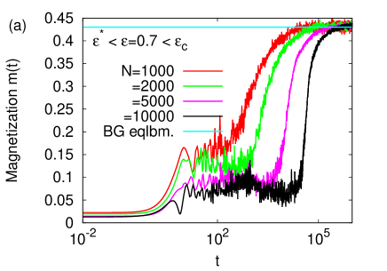
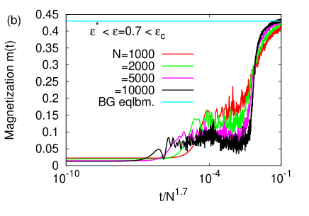
Figure 1: For the model (1), the figures show the magnetization $m(t)$ as a function of time (a), and as a function of time scaled by $N^{1.7}$ (b) in the Vlasov-stable phase ($\epsilon^{\star}<\epsilon<\epsilon_{c}$) for the model (1) at energy density $\epsilon=0.7$. The figures suggest the existence of a QSS with a lifetime scaling with the system size as $N^{1.7}$. Data averaging varies between $5$ histories for the largest system and $10$ histories for the smallest one.

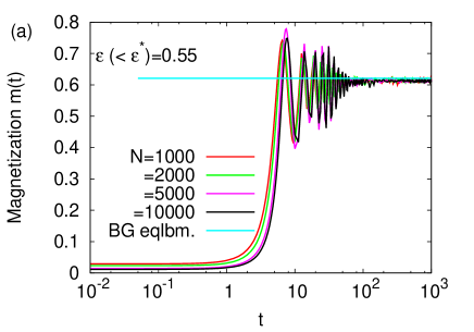
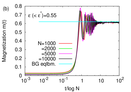
Figure 2: For the model (1), the figures show the magnetization $m(t)$ as a function of time (a), and as a function of time scaled by the logarithm of the system size $N$ (b) in the Vlasov-unstable phase ($\epsilon<\epsilon^{\star}$) at energy density $\epsilon=0.55$. The figures show a fast relaxation from the initial non-magnetized state to BG equilibrium over a timescale $\sim\log N$. Data averaging varies between $5$ histories for the largest system and $10$ histories for the smallest one.

In the next section, we modify the model (1) to include an additional global anisotropy.

III Heisenberg mean-field model with additional global anisotropy

In this section, we consider the system (1) with an additional global anisotropy, and demonstrate the existence of QSSs, similar to the bare model. The analysis is similar to that in the previous section, and therefore, here we briefly outline the main steps. The Hamiltonian of the system is given by

$$H=\frac{1}{2}\sum_{i=1}^{N}\Big{(}p_{\theta_{i}}^{2}+\frac{p_{\phi_{i}}^{2}}{\sin^{2}\theta_{i}}\Big{)}+\frac{1}{2N}\sum_{i,j=1}^{N}\Big{[}1-{\bf S}_{i}\cdot{\bf S}_{j}\Big{]}$$

$$-\frac{K}{2N}(\sum_{i=1}^{N}S_{iz})^{2},$$ (42)

where the last term gives the energy due to a global anisotropy in the magnetization along the $z$ direction. For simplicity, we consider $K>0$ for which the energy is minimized by ordering along the $z$-axis. At the end of this section, we will comment on the case $K<0$.

Following standard procedure (see, e.g., Jain:2007 ), the equilibrium magnetization $\langle m_{z}\rangle$ satisfies

$$\langle m_{z}\rangle=\frac{\int d\theta d\phi\cos\theta\sin\theta e^{\beta(K+1)\langle m_{z}\rangle\cos\theta}}{\int d\theta d\phi\sin\theta e^{\beta(K+1)\langle m_{z}\rangle\cos\theta}}.$$ (43)

Close to the critical point, expanding the above equation to leading order in $\langle m_{z}\rangle$, we get

$$\langle m_{z}\rangle(2-\beta(K+1)\int_{0}^{\pi}d\theta\sin\theta\cos^{2}\theta)=0.$$ (44)

With $\langle m_{z}\rangle\neq 0$, we get the critical temperature $\beta_{c}$ as

$$\beta_{c}=\frac{3}{K+1}.$$ (45)

The critical energy density is

$$\epsilon_{c}(K)=\frac{1}{\beta_{c}}+\frac{1}{2}=\frac{5}{6}+\frac{K}{3};K>0.$$ (46)

The Hamilton equations of motion for the model (42) are obtained from Eqs. (2) - (5) by replacing $m_{z}$ by $(K+1)m_{z}$. The Vlasov equation for the evolution of the single-particle phase space density $f(\theta,\phi,p_{\theta},p_{\phi},t)$ may be derived as in the previous section, and is given by Eq. (7) with $(K+1)m_{z}$ replacing $m_{z}$.

Now, any distribution $f^{(0)}(\theta,\phi,p_{\theta},p_{\phi})=\Phi(e(\theta,\phi,p_{\theta},p_{\phi}))$, with arbitrary function $\Phi$, and $e$ being the single-particle energy,

$$e(\theta,\phi,p_{\theta},p_{\phi})=\frac{1}{2}\Big{(}p_{\theta}^{2}+\frac{p_{\phi}^{2}}{\sin^{2}\theta}\Big{)}$$

$$-m_{x}\sin\theta\cos\phi-m_{y}\sin\theta\sin\phi-(K+1)m_{z}\cos\theta,$$

(47)

is stationary under the Vlasov dynamics. In particular, the non-magnetized state (10) represents a stationary solution of the Vlasov dynamics.

Let us now study the linear stability of the state (10). Noting that when the state is unstable, the system for $K>0$ orders along the $z$ direction, we linearize the Vlasov equation about the state, by writing

$$f(\theta,\phi,p_{\theta},p_{\phi},t)=f^{(0)}+\frac{1}{2\pi}g(\theta,p_{\theta},p_{\phi},\omega)e^{i\omega t},$$ (48)

so that corresponding to the neutral mode $\omega=0$, the quantity $g_{0}=g(\theta,p_{\theta},p_{\phi},0)$ satisfies

$$p_{\theta}\frac{\partial g_{0}}{\partial\theta}+\frac{p^{2}_{\phi}\cos\theta}{\sin^{3}\theta}\frac{\partial g_{0}}{\partial p_{\theta}}$$

$$-\frac{A}{2\pi^{2}}\Big{[}\delta(p_{\theta}+p_{0}(\theta,p_{\phi}))-\delta(p_{\theta}-p_{0}(\theta,p_{\phi}))\Big{]}$$

$$\times(K+1)\widetilde{m}_{z,0}\sin\theta=0.$$ (49)

The above equation is similar to Eq. (24), the only difference being an extra constant factor $(K+1)$ in the term involving $\widetilde{m}_{z,0}$. Consequently, the analysis following Eq. (24) may be similarly carried out in the present case to get

$$a(\theta,p_{\phi})=b(\theta,p_{\phi})=\frac{A(K+1)\widetilde{m}_{z,0}\cos\theta}{2\pi^{2}p_{0}},$$ (50)

which may be combined with Eqs. (25) and (29) to obtain the following equation:

$$\widetilde{m}_{z,0}\Big{[}1-(K+1)\frac{4A}{3}\Big{]}=0.$$ (51)

It then implies that corresponding to the neutral mode, one has $A=A^{\star}=3/(4(K+1))$, which together with Eqs. (13) and (15) give the energy density $\epsilon^{\star}(K)$ corresponding to neutral stability of the stationary state (10) under the linearized Vlasov dynamics:

$$\epsilon^{\star}(K)=\frac{2}{3}+\frac{K}{6};~{}~{}K>0.$$ (52)

Compared to the bare model, we thus see that global anisotropy widens the range of energy $\epsilon^{*}(K)<\epsilon<\epsilon_{c}(K)$ over which the non-magnetized state (10) is linearly stable under the Vlasov dynamics and is hence a QSS. For energies below $\epsilon^{*}(K)$, such a state being linearly unstable exhibits a fast relaxation towards BG equilibrium over a timescale $\sim\log N$, while for energies in the range $\epsilon^{*}(K)<\epsilon<\epsilon_{c}(K)$, it relaxes to BG equilibrium only over a very long timescale growing with the system size as $N^{1.7}$, see Figs. 3 and 4.

For $K<0$, the system will order in the $xy$-plane, and the anisotropy term does not affect the energy. Indeed, an analysis along the same lines as above shows that the energy thresholds $\epsilon^{\star}$ and $\epsilon_{c}$ are equal to the corresponding values for the bare model ($K=0$), and non-magnetized QSSs exist in the range $\epsilon^{\star}<\epsilon<\epsilon_{c}$ ($\epsilon^{*}=2/3,\epsilon_{c}=5/6$).

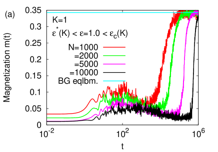
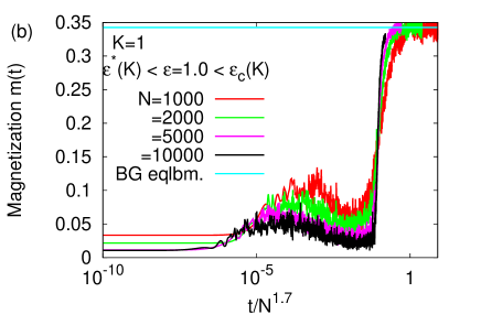
Figure 3: For the model (42), the figures show the magnetization $m(t)$ as a function of time (a), and as a function of time scaled by $N^{1.7}$ (b) in the Vlasov-stable phase ($\epsilon^{\star}(K)<\epsilon<\epsilon_{c}(K)$) for $K=1$ at energy density $\epsilon=1.0$. The figures suggest the existence of a QSS with a lifetime scaling with the system size as $N^{1.7}$. Data averaging varies between $6$ histories for the largest system and $10$ histories for the smallest one.

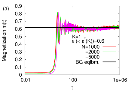
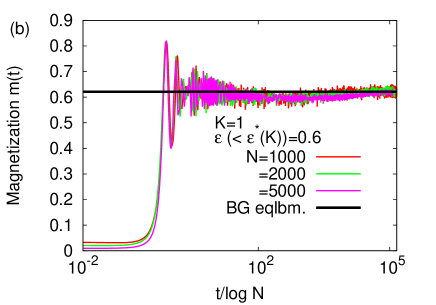
Figure 4: For the model (42), the figures show the magnetization $m(t)$ as a function of time (a), and as a function of time scaled by the logarithm of the system size $N$ (b) in the Vlasov-unstable phase ($\epsilon<\epsilon^{\star}(K)$) for $K=1$ at energy density $\epsilon=0.6$. The figures show a fast relaxation from the initial non-magnetized state to BG equilibrium over a timescale $\sim\log N$. The data shown are for one realization of the dynamics.

IV Conclusions

In this work, we addressed the ubiquity of non-Boltzmann quasistationary states (QSS) in long-range systems. This is done by analyzing the relaxation dynamics of a system of $N$ particles moving on a spherical surface under an attractive Heisenberg-like interaction of infinite range, and evolving under deterministic Hamilton dynamics. In equilibrium, the system exhibits a continuous phase transition from a low-energy magnetized phase to a high-energy homogeneous phase at the energy density $\epsilon_{c}=5/6$. In the limit of infinite $N$, the dynamics of relaxation to equilibrium is described by the Vlasov equation for the temporal evolution of the single-particle phase space distribution. By linearizing the Vlasov equation about a stationary non-magnetized state, our exact solution of the linearized equation shows that within the thermodynamically stable magnetized phase, there exists an energy range $\epsilon^{\star}<\epsilon<\epsilon_{c}$ over which non-magnetized states occur as stable stationary solutions of the Vlasov dynamics, where $\epsilon^{\star}$ corresponds to linear stability threshold of the nonmagnetized states. This leads to the formation of long-lived non-magnetized quasistationary states (QSSs), with a lifetime that we demonstrate on the basis of numerical simulations to be growing algebraically with the system size $N$. For energies below $\epsilon^{\star}$, non-magnetized stationary states are linearly unstable under the Vlasov dynamics, and thus, exhibit a fast relaxation to equilibrium over a timescale growing with the system size as $\log N$. These features remain unaltered on adding a term to the Hamiltonian that accounts for a global anisotropy in the magnetization.

V Acknowledgements

We acknowledge fruitful discussions with Freddy Bouchet, Or Cohen, Thierry Dauxois, and Stefano Ruffo. We are grateful to École Normale Supérieure de Lyon and Korea Institute for Advanced Study for hospitality during our mutual visit when part of this work was done. S. G. acknowledges the CEFIPRA Project 4604-3 and the contract ANR-10-CEXC-010-01 for support. We gratefully acknowledge the support of the Israel Science Foundation (ISF) and the Minerva Foundation with funding from the Federal German Ministry for Education and Research.

References

• (1) Dynamics and Thermodynamics of Systems with Long-Range Interactions (Lecture Notes in Physics vol. 602), edited by T. Dauxois, S. Ruffo, E. Arimondo, and M. Wilkens (Springer-Verlag, Berlin, 2002).
• (2) Dynamics and Thermodynamics of Systems with Long-Range Interactions: Theory and Experiments (AIP Conference Proceedings vol. 970), edited by A. Campa, A. Giansanti, G. Morigi, and F. Sylos Labini (Melville, New York, 2008).
• (3) A. Campa, T. Dauxois, and S. Ruffo, Phys. Rep. 480, 57 (2009).
• (4) Long-Range Interacting Systems, edited by T. Dauxois, S. Ruffo, and L. F. Cugliandolo (Oxford University Press, New York, 2010).
• (5) F. Bouchet, S. Gupta, and D. Mukamel, Physica A 389, 4389 (2010).
• (6) D. Mukamel, in Long-Range Interacting Systems, edited by T. Dauxois, S. Ruffo, and L. F. Cugliandolo (Oxford University Press, New York, 2010) 33.
• (7) J. H. Jeans, Problems of Cosmogony and Stellar Dynamics (Cambridge University Press, Cambridge, 1919).
• (8) T. Padmanabhan, Phys. Rep. 188, 285 (1990).
• (9) D. R. Nicholson, Introduction to Plasma Physics (Krieger Publishing Company, Florida, 1992).
• (10) P. H. Chavanis, in Dynamics and Thermodynamics of Systems with Long-range Interactions (Lecture Notes in Physics vol. 602), edited by T. Dauxois, S. Ruffo, E. Arimondo, and M. Wilkens (Springer-Verlag, Berlin, 2002).
• (11) L. D. Landau and E. M. Lifshitz, Electrodynamics of Continuous Media (Pergamon, London, 1960).
• (12) D. Lynden-Bell and R. Wood, Mon. Not. R. Astron. Soc. 138, 495 (1968).
• (13) W. Thirring, Z. Phys. 235, 339 (1970).
• (14) J. Barré, D. Mukamel, and S. Ruffo, Phys. Rev. Lett. 87, 030601 (2001).
• (15) D. Mukamel, S. Ruffo, and N. Schreiber, Phys. Rev. Lett. 95, 240604 (2005).
• (16) F. Bouchet and J. Barré, J. Stat. Phys. 118, 1073 (2005).
• (17) F. Borgonovi, G. L. Celardo, M. Maianti, and E. Pedersoli, J. Stat. Phys. 116, 1435 (2004).
• (18) F. Borgonovi, G. L. Celardo, A. Musesti, R. Trasarti-Battistoni, and P. Vachal, Phys. Rev. E 73, 026116 (2006).
• (19) F. Bouchet, T. Dauxois, D. Mukamel, and S. Ruffo, Phys. Rev. E 77, 011125 (2008).
• (20) M. Hénon, Annales d’Astrophysique 27, 83 (1964).
• (21) M. Antoni and S. Ruffo, Phys. Rev. E 52, 2361 (1995).
• (22) Y. Y. Yamaguchi, J. Barré, F. Bouchet, T. Dauxois, and S. Ruffo, Physica A 337, 36 (2004).
• (23) A. Campa, A. Giansanti, and G. Morelli, Phys. Rev. E 76, 041117 (2007).
• (24) M. Joyce and T. Worrakitpoonpon, J. Stat. Mech.: Theory Exp. P10012 (2010).
• (25) K. Jain, F. Bouchet, and D. Mukamel, J. Stat. Mech.: Theory Exp. P11008 (2007).
• (26) A. Antoniazzi, D. Fanelli, J. Barré, P-H. Chavanis, T. Dauxois, and S. Ruffo, Phys. Rev. E 75, 011112 (2007).
• (27) Y. Levin, , R. Pakter , F. B. Rizzato , T. N. Teles, F. P. da C. Benetti, Phys. Rep. (in press).
• (28) W. Ettoumi and M.-C. Firpo, Phys. Rev. E 87, 030102(R) (2013).
• (29) J. Barré, T. Dauxois, G. De Ninno, D. Fanelli, and S. Ruffo, Phys. Rev. E 69, 045501(R) (2004).
• (30) R. Kawahara and H. Nakanishi, J. Phys. Soc. Jpn. 75, 054001 (2006).
• (31) F. Baldovin and E. Orlandini, Phys. Rev. Lett. 96, 240602 (2006).
• (32) F. Baldovin and E. Orlandini, Phys. Rev. Lett. 97, 100601 (2006).
• (33) F. Baldovin, P. H. Chavanis, and E. Orlandini, Phys. Rev. E 79, 011102 (2009).
• (34) S. Gupta and D. Mukamel, Phys. Rev. Lett. 105, 040602 (2010).
• (35) S. Gupta and D. Mukamel, J. Stat. Mech.: Theory Exp. P08026 (2010).
• (36) P. H. Chavanis, F. Baldovin, and E. Orlandini, Phys. Rev. E 83, 040101(R) (2011).
• (37) F. D. Nobre and C. Tsallis, Phys. Rev. E 68, 036115 (2003).
• (38) F. D. Nobre and C. Tsallis, Physica A 344, 587 (2004).
• (39) M. Kac, G. E. Uhlenbeck, and P. C. Hemmer, J. Math. Phys. 4, 216 (1963).
• (40) W. Braun and K. Hepp, Comm. Math. Phys. 56, 101 (1977).
• (41) Note that the initial condition referred to as water-bag in Refs. Nobre:2003 ; Nobre:2004 is very different from the state (10).
• (42) A. Figueiredo, T. M. Rocha Filho, A. E. Santana, M. A. Amato, e-print:arXiv:1305.4417.