The orientation dependence of quasar spectral energy distributions

Abstract

We investigate the orientation dependence of the spectral energy distributions in a sample of radio-loud quasars. Selected specifically to study orientation issues, the sample contains 52 sources with redshifts in the range $0.16<z<1.4$ and measurements of radio core dominance, a radio orientation indicator. Measured properties include monochromatic luminosities at a range of wavelengths between the infrared and X-rays, integrated infrared luminosity, spectral slopes, and the covering fraction of the obscuring circumnuclear dust. We estimate dust covering fraction assuming that the accretion disk emits anisotropically and discuss the shortcomings and technical difficulties of this calculation. Luminosities are found to depend on orientation, with face-on sources factors of a $2-3$ brighter than more edge-on sources, depending on wavelength. The degree of anisotropy varies very little with wavelength such that the overall shape of the spectral energy distribution does not vary significantly with orientation. In the infrared, we do not observe a decrease in anisotropy with increasing wavelength. The spectral slopes and estimates of covering fraction are not significantly orientation dependent. We construct composite spectral energy distributions as a function of radio core dominance and find that these illustrate the results determined from the measured properties.

1 introduction

Quasars are notable for emitting their substantial luminosity over the entire electromagnetic spectrum. A variety of physical processes, both thermal and non-thermal, and environments, with gas at a range of temperatures and distances from the central engine, are required to produce the observed quasar spectral energy distributions (SEDs, for a review see Wilkes, 2004). Quasars are too distant to be resolved spatially (except the radio jets that can be seen on the largest scales), so information about their internal structures must be gathered indirectly. As a result, observed properties of the SED are used to infer much about the physical nature of quasars and a good understanding of the orientation dependence of these observations is necessary.

Generally speaking, all quasar SEDs exhibit similar emission components. The most prominent feature is the peak in emission at optical/ultraviolet (UV) wavelengths, called the “Big Blue Bump.” This feature can be produced by thermal emission from the accretion disk surrounding the central supermassive black hole, where gas attains a range of temperatures, typically around $\sim 10^{4-5}$ K.

A corona surrounding the accretion disk is capable of up-scattering photons to X-ray energies, producing one component of the observed high-energy SED. Radio-loud (RL) quasars have an additional jet-linked component to their X-ray emission (e.g., Kembhavi, Feigelson & Singh, 1986).

The mid-infrared (MIR) portion of the SED is thought to be produced by a body of circumnuclear dust, hereafter referred to as a dusty torus. The dust intercepts some fraction of the optical/UV emission from the accretion disk, reprocesses it, and re-emits at a range of wavelengths in the IR. The torus is central to the unification of active galactic nuclei (AGN) that are observed with both broad and narrow emission lines (Type 1) and those that show only narrow emission lines (Type 2) (Antonucci, 1993). In this picture, emission from the narrow line region is observed in both classes of AGN, but Type 1 sources are seen more face-on with a line of sight down into the central nucleus of the AGN where the broad lines are emitted. Type 2 sources are seen more edge-on and the dusty torus blocks this view.

The radio region of the SED, which is primarily produced by a jet, is where RL and radio-quiet (RQ) sources distinguish themselves. For similar optical emission, RL quasars can be many orders of magnitude brighter in the radio than RQ quasars.

The only well-established method of determining orientation in quasars depends on the anisotropy of the radio emission. Radio orientation indicators rely on the beaming of the radio jet emission to estimate orientation (e.g., Wills & Brotherton, 1995). Ideally, an anisotropically beamed quantity is normalized to one that is known to be emitted more isotropically, thus indicating the intrinsic power of the source. Radio core dominance, the ratio of the of the radio core luminosity to the radio lobe luminosity at rest-frame 5 GHz, is one such orientation indicator. Ghisellini et al. (1993) demonstrate that the radio core dominance parameter, log$\,R=\textrm{log}\,\left(\frac{L_{core}}{L_{ext.}}\right)$, tracks the viewing angle obtained from high-resolution radio maps that show superluminal motion in the radio jets of approximately 40 objects (see Wills & Brotherton, 1995, for an updated figure). This method is incredibly powerful, but the technique is limited by the fact that it can be applied to only the 10% of AGN that are RL because it depends exclusively on observations of the radio structures.

At least in RL quasars, the behavior of the radio emission as a function of orientation is well understood. In some other wavelength regimes, the degree of anisotropy with which the SED is emitted is either known or can be anticipated based on physical models. In the optical/UV early radiative transfer modeling of geometrically thin accretion disks suggests that the flux may vary by a factors of a few between edge-on and face-on sources (e.g., Laor & Netzer, 1989). More recent results from Nemmen & Brotherton (2010), who use the accretion disk models of Hubeny et al. (2000) that account for limb darkening and relativistic effects, show a similar degree of anisotropy in the optical/UV for typical quasar input parameters.

The emission from the dusty torus can also be reproduced with some success via radiative transfer modeling. In early models, most notably those of Pier & Krolik (1992), the dust is distributed smoothly throughout the torus. This induces a significant orientation dependence, over an order of magnitude difference in the flux from edge-on and face-on sources at 10 $\mu$m. The anisotropy arises from the fact that the torus is optically thick and the hot dust near the central nucleus of the AGN is revealed at more face-on inclinations, where it contributes significantly to the MIR emission. Later models adopt a clumpy distribution for the dust (Nenkova et al., 2008). In this case, the inner faces of the optically thick dust clouds are illuminated but can be observed from a wider range of inclinations extending to more edge-on views. As a result, the models of Nenkova et al. (2008) are capable of producing anisotropic emission in the MIR, but the orientation dependence can vary depending on the input parameters and is generally much less significant than for the smooth torus models. The clumpy torus models are generally considered to be more realistic than those with a smooth dust distribution and have been shown to reproduce the observed near-infrared (NIR) and MIR SED well, even at high spatial resolution (e.g., Ramos Almeida et al., 2011; Alonso-Herrero et al., 2011).

The SED atlas of Shang et al. (2011), which includes the most detailed and up-to-date SEDs for 85 AGN and a subsample designed for studying orientation, provides an ideal opportunity to investigate the orientation dependence of quasar emission at all wavelengths. Some properties have already been investigated for this sample in previous work. Runnoe et al. (2013) demonstrate that the optical/UV monochromatic luminosities depend on radio core dominance. The X-ray-to-optical spectral index, which indicates the relative strength of the X-ray emission compared to the Big Blue Bump, does not depend on orientation (Runnoe et al. submitted). The aim of this work is to compile these known dependencies and provide a new analysis of the orientation dependencies of the IR emission and the covering fraction of the dusty torus as well as construct composite SEDs to give a full picture of the orientation dependence of quasar SEDs. The orientation dependence of the radio is well established, so we use this dependence to indicate orientation rather than include it in our analysis.

This investigation is structured as follows: in Section 2 we discuss the sample and measurements. The presentation of known orientation dependencies as well as new analysis of the IR and the creation of composite SEDs is detailed in Section 3. The results are discussed in the context of previous work in Section 4 and we summarize this work in Section 5. Throughout this work we use a cosmology with $H_{0}=70$ km s^-1 Mpc^-1, $\Omega_{\Lambda}=0.7$, and $\Omega_{m}=0.3$.

2 Sample, Data, and Measurements

For this investigation we use the RL subsample of the Shang et al. (2011) SED atlas. This sample is ideal for investigating orientation dependencies: objects are selected to have similar extended radio luminosity, which is thought to be emitted isotropically. As a result of this selection, objects included in the sample are intrinsically similar but viewed at different angles. This isolates the orientation effects that are of interest and minimizes differences caused by other parameters that might affect the SED, increasing our ability to discern statistically significant differences in the SEDs and their properties as a function of orientation. The blazars originally included by Shang et al. have been removed. The total sample of 52 objects, with redshifts in the range $0.16<z<1.4$, is discussed in Runnoe et al. (2013).

Radio through X-ray SEDs are available for all of the objects in this sample, with varying levels of completeness. Shang et al. (2011) describes the construction of the SEDs in detail, but we briefly describe the source of relevant data here.

X-ray data are available for 34 out of 52 objects (65%). Observations are from the Chandra X-ray Observatory, XMM-Newton, or ROSAT and are tabulated from the literature in Shang et al. (2011). In order to quantify the shape of the X-ray spectra for inclusion in the SEDs, Shang et al. (2011) use a power law or broken power law of the form $f_{\nu}=f_{0}E^{\alpha}$, where $f_{0}$ is the flux density at 1 keV, $E$ is the energy in keV, and $\alpha$ is the power-law spectral index. They tabulate these parameters and use errors on the X-ray spectral index to determine uncertainty in this part of the SED.

Optical and UV spectrophotometry were obtained quasi-simultaneously for the entirety of this sample. The sample was targeted with the Hubble Space Telescope (HST) as part of an early HST program and those observations were followed, usually within weeks, by optical observations from Kitt Peak National Observatory or McDonald Observatory.

IR coverage for the full SED sample comes from the 2 Micron All Sky Survey (2MASS; Skrutskie et al., 2006) and the Spitzer Space Telescope. The RL subsample is rather poorly represented with only 9 objects having Spitzer coverage so we instead tabulate IR data from the Wide-field Infrared Survey Explorer (WISE; Wright et al., 2010). WISE covers four bands (W$1-4$) at 3.4, 4.6, 12, and 22 $\mu$m and is available for 42 (81%) objects in the RL sample. Using sources in the full SED sample that have both WISE and Spitzer coverage, Runnoe, Brotherton & Shang (2012b) verify that there are likely no significant variability issues associated with including the WISE data as emission varies by less than $5-10\%$ in the $4-5$ years between Spitzer and WISE.

Radio fluxes at multiple frequencies are available for this sample, tabulated from high-quality surveys and the literature by Shang et al. (2011). Not all sources are resolved in the original SED radio data, so Runnoe et al. (2013) tabulate additional radio core and extended fluxes from the literature in order to calculate radio core dominance.

Shang et al. (2011) have applied two corrections during the construction of the SEDs. First, there is a correction for host emission that can contaminate emission from the AGN at optical and NIR wavelengths. Second is the correction for Galactic reddening to the emission at optical-to-far-ultraviolet wavelengths.

Optical, UV, and X-ray monochromatic luminosities have already been measured for this sample and are presented in Runnoe, Brotherton & Shang (2012a). Here we add measurements of the monochromatic luminosity at 3, 8, and 12 $\mu$m, calculated from magnitudes available in the WISE All-Sky Data Release. There is a known discrepancy that arises between red and blue calibrator stars for the WISE magnitudes. Described in detail in Wright et al. (2010), we correct this issue by adding $+17\%$ and $-9\%$ in flux to the W3 and W4 bands, respectively. We then k-correct the luminosities to 3, 8, and 12 $\mu$m following the formalism of Stocke et al. (1992) and using the observed W2, W3, and W4 fluxes. IR spectra of quasars are typically well approximated by a power law, so in order to obtain the slope for the k-correction, we fit a power law to all four WISE bands in log space and verify visually that this is reasonable.

In addition to these monochromatic luminosities, we also calculate an integrated luminosity in the MIR, $L$(MIR). Similar to Ma & Wang (2013), we integrate a power law between the first and fourth WISE points over MIR wavelengths in order to determine this quantity. This practice is intended to determine the emission from hot dust, but contamination from other sources can be an issue. We select the wavelength range of rest-frame $3-12$ $\mu$m in order to minimize contributions from the accretion disk or cool dust heated by star formation in the host galaxy. Using the Type 1 SED from Silva, Maiolino & Granato (2004), Maiolino et al. (2007) determine that the monochromatic luminosity at 6.7 $\mu$m must be scaled up by a factor of $\sim 2.7$ in order to estimate the integrated IR luminosity in the range $4-10$ $\mu$m. We find a smaller correction of 1.8 on average, but for a different wavelength region.

We measure spectral indices between the X-ray and optical and the optical and IR for this sample. The slope between the flux at 2500 Å and 2 keV, $\alpha_{ox}$, has already been measured for this sample by Runnoe et al. (submitted) and we calculate the slope between the flux at 2500 Å and 12 $\mu$m, $\alpha_{oIR}$. Both spectral indices are calculated directly from the data using the expression in Steffen et al. (2006) with appropriate fluxes and frequencies.

We estimate covering fraction using a method similar to DiPompeo et al. (2013). Calderone, Sbarrato & Ghisellini (2012) derive the following limits on the covering fraction of the dusty torus (their equation 10):

$$\frac{c^{2}}{1+c}<R<c^{2},$$ (1)

where $c$ is the covering fraction and $R$ is the observable $L(\textrm{MIR})/L_{bol}$. This estimate accounts for the fact that the accretion disk luminosity is anisotropically emitted, although only via a geometric $\cos(\theta)$ effect. We determine covering fraction estimates for our sample by inverting Equation 1 to give limits on the covering fraction as a function of $R$ and averaging these upper and lower limits. Bolometric luminosity is taken from Runnoe, Brotherton & Shang (2012a) and is determined by integrating the SED between 1 $\mu$m and 2 keV or, when the complete SED is not observed, from the recommended bolometric correction at 1450 Å derived in that work. By excluding the IR emission in the bolometric luminosity integration, we avoid issues of double counting the IR photons.

Radio orientation indicators for this sample are presented in Runnoe et al. (2013). Radio core dominance is calculated by k-correcting the luminosities from the radio core and extended radio lobes to rest-frame 5 GHz assuming slopes of $\alpha=0$ and $\alpha=-0.7$, respectively. A measurement of radio core dominance requires that the source be resolved in the radio map. The power of this method is that the core and lobe luminosities can be properly ascribed to their respective sources with reasonable certainty.

Table LABEL:tab:measurements contains all luminosities, spectral indices, radio core dominance, and covering fraction measurements for this sample.

Table 1: Measurements

Object	Lbol	$\,\lambda L_{\lambda}$(2 keV)	$\,\lambda L_{\lambda}$(1450 Å)	$\,\lambda L_{\lambda}$(2500 Å)	$\,\lambda L_{\lambda}$(5100 Å)	$\,\lambda L_{\lambda}$(3 $\mu$m)	$\,\lambda L_{\lambda}$(8 $\mu$m)	$\,\lambda L_{\lambda}$(12 $\mu$m)	L(MIR)	$\alpha_{ox}$	$\alpha_{oIR}$	log$\,R$	$c$
	ergs s-1	ergs s-1	ergs s-1	ergs s-1	ergs s-1	ergs s-1	ergs s-1	ergs s-1	ergs s-1				%
3C 110	46.99		46.43	46.24	45.99							$-$0.249
3C 175	46.91		46.34	46.31	46.11	45.88	45.73	45.74	46.03		$-$0.66	$-$1.836	40
3C 186	46.66		46.07	45.97	45.79	45.67	45.71	45.68	45.94		$-$0.83	0.060	48
3C 207	46.28		45.65	45.65	45.48	45.31	45.44	45.43	45.68		$-$0.87	$-$0.393	56
3C 215	45.77	44.83	45.02	44.93	44.94	44.96	44.88	45.00	45.26	$-$1.04	$-$1.04	$-$1.521	64
3C 232	46.36	44.50	45.87	45.94	45.72	45.36	45.33	45.38	45.66	$-$1.55	$-$0.67	0.641	50
3C 254	46.17	44.10	45.63	45.55	45.36					$-$1.56		$-$1.722
3C 263	46.81	43.75	46.33	46.23	46.01	45.92	45.84	45.86	46.13	$-$1.95	$-$0.78	$-$0.912	51
3C 277.1	45.61	44.30	45.04	44.89	44.67	44.65	44.86	44.88	45.11	$-$1.23	$-$0.99	$-$1.425	65
3C 281	46.23	45.06	45.68	45.58	45.32	45.31	45.14	45.18	45.47	$-$1.20	$-$0.76	$-$0.967	46
3C 288.1	46.61		46.01	45.90	45.62	45.55	45.63	45.77	46.01		$-$0.92	$-$2.169	56
3C 334	46.44	44.55	46.00	45.90	45.58	45.58	45.58	45.74	45.98	$-$1.52	$-$0.90	$-$0.648	68
3C 37	46.18	45.02	45.28	45.26	44.89	45.50	45.44	45.41	45.69	$-$1.09	$-$1.09	$-$0.433	66
3C 446	47.01	46.25	46.19	46.28	46.43					$-$1.01		1.528
3C 47	45.97	44.80	45.27	45.10	44.88	45.50	45.47	45.46	45.73	$-$1.11	$-$1.22	$-$1.286	92
4C 01.04	45.44	44.56	44.43	44.56	44.69	44.75	44.92	44.93	45.17	$-$1.00	$-$1.22	$-$0.621	90
4C 06.69	47.30	46.32	46.73	46.59	46.43	46.47	46.48	46.47	46.72	$-$1.11	$-$0.93	2.101	58
4C 10.06	46.48	45.30	45.85	45.73	45.47	45.40	45.36	45.33	45.61	$-$1.17	$-$0.76	$-$0.658	39
4C 12.40	46.17		45.53	45.34	45.13	45.07	45.03	45.05	45.33		$-$0.83	$-$1.163	41
4C 19.44	46.91	45.76	46.30	46.21	45.99	45.90	45.96	46.05	46.29	$-$1.17	$-$0.90	0.427	55
4C 20.24	46.92	45.81	46.22	46.17	45.95	45.98	46.01	46.03	46.28	$-$1.14	$-$0.92	$-$0.499	54
4C 22.26	46.59	44.91	45.83	45.70	45.52	45.44	45.61	45.62	45.85	$-$1.30	$-$0.95	$-$1.028	47
4C 30.25	46.27		45.64	45.53	45.13	45.28	45.31	45.27	45.54		$-$0.84	$-$1.740	48
4C 31.63	46.61	45.00	46.21	46.03	45.61	45.58	45.54	45.46	45.75	$-$1.39	$-$0.66	0.979	40
4C 39.25	46.91	45.63	46.25	46.15	45.97	45.88	45.88	45.83	46.09	$-$1.20	$-$0.81	$-$2.220	43
4C 40.24	46.60	45.47	45.96	45.87	45.74	45.83	45.96	45.78	46.05	$-$1.15	$-$0.95	$-$0.477	60
4C 41.21	46.75	45.42	46.27	46.01	45.64	45.84	45.75	45.70	45.97	$-$1.23	$-$0.81	$-$0.477	45
4C 49.22	45.99	44.96	45.21	45.14	44.84	45.47	45.51	45.49	45.75	$-$1.07	$-$1.21	$-$0.046	92
4C 55.17	46.46	45.16	45.83	45.78	45.72	45.92	46.00	45.98	46.24	$-$1.24	$-$1.12	1.238	95
4C 58.29	47.20	45.09	46.73	46.58	46.42	46.18	46.21	46.16	46.42	$-$1.57	$-$0.76	$-$1.561	45
4C 64.15	46.73		46.14	46.03	45.98							$-$1.793
4C 73.18	46.40	44.98	45.80	45.77	45.55	45.63	45.57	45.59	45.87	$-$1.30	$-$0.89	1.265	62
B2 0742+31	46.46	45.34	45.89	45.93	45.77	45.86	45.75	45.83	46.10	$-$1.22	$-$0.94	0.360	78
B2 1351+31	46.66		46.07	45.94	45.81	45.53	45.65	45.63	45.87		$-$0.81	$-$0.474	44
B2 1555+33	46.21		45.57	45.44	45.39	45.44	45.39	45.27	45.57		$-$0.90	0.212	54
B2 1611+34	47.06		46.50	46.35	46.29	46.03	46.11	46.16	46.41		$-$0.89	0.014	53
MC2 0042+101	45.68		44.99	45.04	44.94	44.94	44.81	44.72	45.04		$-$0.81	$-$0.821	54
MC2 1146+111	46.29		45.66	45.71	45.52	45.41	45.29	45.05	45.39		$-$0.60	$-$1.311	38
OS 562	46.74	45.03	46.21	46.03	45.82	45.64	45.64	45.65	45.92	$-$1.38	$-$0.78	0.891	43
PG 1100+772	46.46	45.25	45.90	45.74	45.44	45.43	45.34	45.32	45.61	$-$1.19	$-$0.75	$-$1.095	41
PG 1103-006	46.30		45.67	45.61	45.30							$-$0.391
PG 1226+023	46.96	45.70	46.45	46.34	45.97	45.96	45.78	45.74	46.05	$-$1.25	$-$0.64	0.643	38
PG 1545+210	45.93	44.62	45.39	45.32	45.07	45.22	45.05	45.05	45.35	$-$1.27	$-$0.84	$-$1.750	58
PG 1704+608	46.49	44.74	45.91	45.86	45.72	45.85	45.72	45.81	46.08	$-$1.43	$-$0.97	$-$1.385	73
PG 2251+113	46.35		45.73	45.73	45.53	45.59	45.41	45.37	45.69		$-$0.79	$-$2.501	52
PKS 0112-017	46.88	45.47	46.44	46.30	46.07					$-$1.32		$-$0.569
PKS 0403-13	46.36	45.51	45.69	45.65	45.53					$-$1.05		1.696
PKS 0859-14	47.22		46.68	46.56	46.45							1.404
PKS 1127-14	47.15	46.31	46.50	46.40	46.21					$-$1.04		1.950
PKS 1656+053	47.06	46.14	46.44	46.36	46.26	46.23	46.29	46.27	46.51	$-$1.08	$-$0.94	$-$0.017	61
PKS 2216-03	46.95		46.38	46.39	46.31							0.922
TEX 1156+213	46.01		45.36	45.26	45.00	45.10	45.00	44.89	45.20		$-$0.78	$-$1.228	43

• Note $-$ All luminosities are in log space.

3 Analysis

We investigate the orientation dependence of a variety of properties of the SED. The analysis consists of three parts. The first part is a rank correlation analysis of the orientation dependence of properties of the SED. Second, we investigate in particular the orientation dependence of the covering fraction of the dusty torus. Finally, we construct composite SEDs in order to demonstrate visually the differences in the SED with orientation.

3.1 Properties of the SED

In order to quantify the orientation dependence of the measured luminosities and spectral slopes, we present the Spearman Rank (RS) correlations between these and radio core dominance in Table 2. For each correlation we tabulate the number of objects (which may be fewer than the total sample size if data are not available), the RS statistic, $\rho$, and the probability, $P$, of achieving the observed distribution of points by chance. We define a significant correlation as one having a value of $P$ that is 0.01 or less and a marginally significant correlation as having a value of $P$ that is 0.05 or less. In Table 2 these correlations, which we take to indicate an orientation dependence, are highlighted in bold. The correlations between the luminosities and radio core dominance are illustrated in Figure 1 and those between spectral slopes and radio core dominance are illustrated in Figure 2. In these figures, average values of each parameter are presented with the 1$\sigma$ dispersion in the X and Y directions to indicate typical values for core-dominated (log $R\geq 0$) and and lobe-dominated (log $R<0$) sources. These average values are tabulated in Table 3 and indicate the average degree of anisotropy at each wavelength.

Table 2: Correlations with orientation

Param 1	Param 2	N	$\rho$	P
$\lambda$Lλ(2 keV)	log $R$	34	$0.521$	$\boldsymbol{0.002}$
$\lambda$Lλ(1450 Å)	log $R$	52	$0.344$	$\boldsymbol{0.013}$
$\lambda$Lλ(2500 Å)	log $R$	52	$0.390$	$\boldsymbol{0.004}$
$\lambda$Lλ(5100 Å)	log $R$	52	$0.387$	$\boldsymbol{0.005}$
$\lambda$Lλ(3 $\mu$m)	log $R$	42	$0.343$	$\boldsymbol{0.026}$
$\lambda$Lλ(8 $\mu$m)	log $R$	42	$0.358$	$\boldsymbol{0.020}$
$\lambda$Lλ(12 $\mu$m)	log $R$	42	$0.316$	$\boldsymbol{0.041}$
L(MIR)	log $R$	42	$0.336$	$\boldsymbol{0.030}$
$\alpha_{ox}$	log $R$	34	$0.281$	$0.107$
$\alpha_{oIR}$	log $R$	42	$-0.082$	$0.607$
$c$	log $R$	42	$0.141$	$0.373$

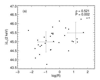
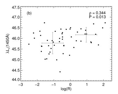
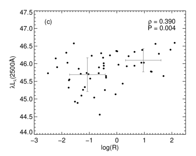
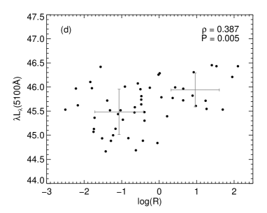
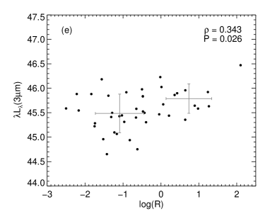
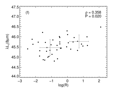
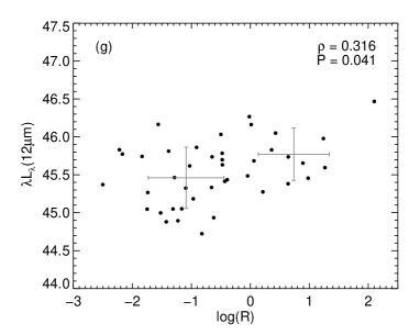
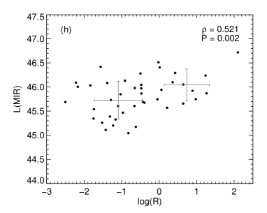
Figure 1: Monochromatic and integrated IR luminosities versus radio core dominance, an orientation indicator. The Spearman Rank correlation coefficient and associated probability of finding these distributions of points by chance are listed in the upper right corner of each plot. Gray crosses indicate the average values for core-dominated (log $R\geq 0$) and and lobe-dominated (log $R<0$) sources with 1$\sigma$ dispersion in the X and Y directions. The orientation dependence is marginally significant at 1450 Å and at all IR wavelengths and significant at 2 keV, 2500 Å, and 5100 Å.

Table 3: Average parameter values

Parameter	Core	Lobe	Core/Lobe
log$\,\lambda$Lλ(2 keV)	45.49$\pm$0.59	44.99$\pm$0.56	3.15
log$\,\lambda$Lλ(1450 Å)	46.17$\pm$0.35	45.78$\pm$0.51	2.46
log$\,\lambda$Lλ(2500 Å)	46.10$\pm$0.33	45.69$\pm$0.48	2.55
log$\,\lambda$Lλ(5100 Å)	45.94$\pm$0.35	45.49$\pm$0.47	2.85
log$\,\lambda$Lλ(3 $\mu$m)	45.79$\pm$0.30	45.49$\pm$0.39	2.01
log$\,\lambda$Lλ(8 $\mu$m)	45.77$\pm$0.32	45.47$\pm$0.40	2.00
log$\,\lambda$Lλ(12 $\mu$m)	45.77$\pm$0.35	45.46$\pm$0.40	2.05
L(MIR)	46.04$\pm$0.33	45.73$\pm$0.39	2.06
$\alpha_{ox}$	$-$1.23$\pm$0.16	$-$1.26$\pm$0.22	0.97
$\alpha_{oIR}$	$-$0.85$\pm$0.14	$-$0.89$\pm$0.15	0.95
$c$	0.57$\pm$0.16	0.56$\pm$0.15	1.01

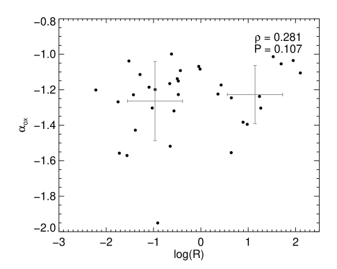
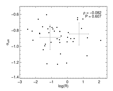
Figure 2: The spectral slopes $\alpha_{ox}$ and $\alpha_{oIR}$ and radio core dominance. Neither shows a statistically significant orientation dependence. The Spearman Rank correlation coefficient and associated probability of finding these distributions of points by chance are listed in the upper right corner of each plot. Gray crosses indicate the average values for core-dominated (log $R\geq 0$) and and lobe-dominated (log $R<0$) sources with 1$\sigma$ dispersion in the X and Y directions.

Of the monochromatic luminosities,the X-ray luminosity at 2 keV and the 2500 and 5100 Å luminosities show a significant dependence on radio core dominance. The UV and IR luminosities show marginally significant dependencies. In general, face-on sources are brighter than more edge-on sources by factors of $2-3$ depending on wavelength, but the degree of anisotropy at each wavelength is such that the shape of the SED changes very little with orientation. We also find that neither the optical-X-ray nor optical-IR spectral slopes show a statistically significant orientation dependence. Some of these results are previously known and will be discussed further in Section 4.

In the IR it is common to compare the orientation dependencies as a function of wavelength. The significance of the correlation is similar at 3, 8, and 12 $\mu$m and, comparing the degree of anisotropy between the core-dominated and lobe-dominated sources, there is no significant change with wavelength.

3.2 Covering fraction

We have estimated the covering fraction from the ratio of the integrated luminosity in the MIR to the bolometric luminosity, what is essentially the fraction of the bolometric luminosity emitted by the accretion disk that is reprocessed into the IR by a dusty torus. We find a mean covering fraction for the total sample of $0.56\pm 0.15$ (corresponding to an opening angle from the jet axis of $56^{\circ}$), where the uncertainty is the standard deviation of the covering fractions measured in this sample.

The correlation between radio core dominance and estimates of covering fraction is presented in Table 2 and illustrated in Figure 3. We find that estimates of the covering fraction of the dusty torus do not correlate with radio core dominance. This is not surprising given the similar orientation dependencies of the 12 $\mu$m and 1450 Å luminosities, where the 1450 Å luminosity is a proxy for the bolometric luminosity. Though not identical, the orientation dependencies of the IR and UV luminosities are very similar.

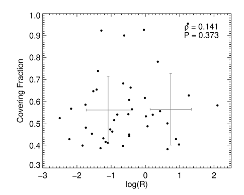
Figure 3: The covering fraction of the dusty torus and radio core dominance. The covering fraction does not significantly depend on orientation. The Spearman Rank correlation coefficient and associated probability of finding these distributions of points by chance are listed in the upper right corner of the plot. Gray crosses indicate the average values for core-dominated (log $R\geq 0$) and and lobe-dominated (log $R<0$) sources with 1$\sigma$ dispersion in the X and Y directions.

3.3 Composite SEDs

Making composites is a powerful way of visually demonstrating the orientation dependence of the SED. We create two composites for sources with log $R<0$ and log $R>0$ following the method of Shang et al. (2011).

The construction process is as follows. Unlike Shang et al. (2011), we do not normalize the SEDs before constructing the composites because the sample is selected on extended radio luminosity to include intrinsically similar objects with varying orientation. The first step is to bin the data. Each bin will contribute one point to the final SED at the center frequency of the bin and we use same bins for the creation of each composite SED. Our bins are similar and sometimes identical to those used in Shang et al. (2011). We use the distribution of points for all objects to be included in the composite to manually determine the binning. In the optical/UV and X-ray where the SEDs include continuous spectra, it is straightforward to create bins of uniform width across the relevant frequency range. In the radio and IR where the data coverage is less consistent, bins are determined manually. In these cases, we try to exclude regions without data and create similar width bins over the remaining frequency space.

To create the final composite, sources with multiple points in one bin are rebinned and then the data are median combined. This method is chosen so that each source is weighted equally and to reject outliers and prevent individual objects from dominating features of the final composite. In a final pass, we evaluate the number of objects contributing data in each bin and exclude any points that are determined by fewer than 8 sources. The final composite SEDs are shown in Figure 4 along with panels showing the number of sources and standard deviation in each bin.

In the absence of complete data coverage there is no perfect way to construct composite SEDs. The partial data coverage in the IR in particular means that those points in the final composite have larger uncertainties associated with them. However, the composites are intended to be help the reader visualize the results of the correlation analysis so it is not critical to know each point with high precision.

Figure 4: Composite spectra binned by log $R$, a radio orientation indicator. For each composite we also include a panel with the number of sources contributing data to each bin and the standard deviation of the data in each bin.

The composites serve to illustrate many of the results found in the rank correlation analysis. Figure 5 shows the two composites plotted together over the full frequency range. In general, the face-on composite is brighter than the edge-on composite and the optical-to-X-ray and optical-to-IR slopes are similar between both composites. It is particularly clear here that the shape of the SED is relatively constant with orientation. Figure 6 shows a comparison of the composites in the IR-through-X-ray spectral regime. In the IR, there is no clear change in the orientation dependence going to lower frequency.

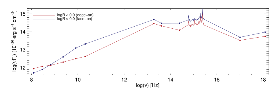
Figure 5: Composite SEDs compared over the full frequency range. The face-on composite is brighter and, most notably, the shape of the SED is similar in all three composites.

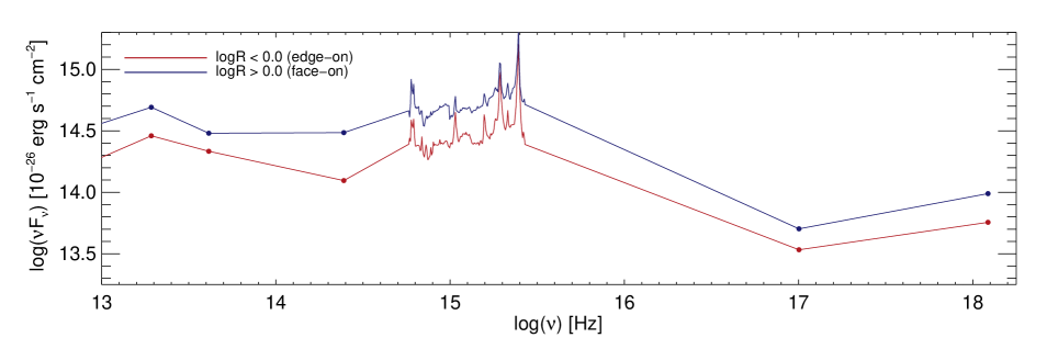
Figure 6: Composite SEDs compared in the IR-to-X-ray regime. The face-on composite is brighter and there is no obvious decrease in the difference between the face-on and edge-on composites with increasing wavelength.

4 Discussion

The orientation dependence of quasar emission has long been of interest. As a result, many of these results are known in the literature and we discuss them here in the context of previous work.

4.1 X-ray and optical/UV luminosities

The orientation dependence of the X-ray monochromatic luminosity at 2 keV is known (Jackson et al., 1989) and has an accepted explanation. RL quasars are known to have more X-ray flux than RQ quasars, typically an excess of a factor of 3 but potentially a factor of 10 or more for the most RL sources (Miller et al., 2011). This X-ray emission has two components from different origins. One component, that is likely similar to what is observed in RQ quasars, is consistent with an origin related to a hot corona and the accretion disk (Miller et al., 2011). There is also a jet-linked component (e.g., Kembhavi, Feigelson & Singh, 1986; Shastri et al., 1993; Miller et al., 2011) that is stronger in objects viewed more face-on (Worrall et al., 1987) and causes objects that are more RL to have flatter X-ray spectra (Wilkes & Elvis, 1987; Shastri, 1991). As our sample is exclusively RL, it is possible that at least some of the observed orientation dependence is the result of a beamed X-ray component. Without the ability to separate the X-ray emission from a hot corona and a jet-linked mechanism, it is not possible to conclusively attribute the observed orientation dependence to either source. In particular, this means that for the hot corona, we can’t address the degree of anisotropy.

The orientation dependence of the optical/UV luminosities is known and has been demonstrated for this sample before by Runnoe et al. (2013). Browne & Wright (1985) and others have shown that core-dominated sources (viewed more face-on, log $R>0$) are optically brighter than lobe-dominated sources. Furthermore, the degree of anisotropy observed in this sample is generally consistent with the amount, typically a few tenths of a decade between edge-on and face-on sources, expected from accretion disk models (Laor & Netzer, 1989; Nemmen & Brotherton, 2010).

4.2 IR luminosities

Observations are generally consistent with the level of orientation dependence expected from a clumpy torus as opposed to a smooth one (which would have a very strong degree of anisotropy of an order of magnitude or more), but there is variation in the details. In general, the approach to evaluate the degree of anisotropy in the MIR emission has been to compare the MIR emission normalized to the intrinsic AGN power (usually an X-ray or radio luminosity) in Type 1 and Type 2 sources, which are thought to be viewed face and edge-on, respectively, in the unified model.

Based on this type of analysis, some investigations conclude that the MIR emission from AGN is relatively isotropic. Comparisons between Type 1 and Type 2 Seyferts reveals no difference in the relation between the MIR and X-ray luminosities, indicating that the MIR emission is similar in face-on and edge-on objects and therefore is relatively isotropically emitted (Horst et al., 2008; Levenson et al., 2009). However, in the case of Levenson et al. (2009), there are significant uncertainties on the luminosities used to draw this conclusion.

On the other hand, some studies find that the MIR is emitted anisotropically. A comparison of the IR SEDs of RL quasars and radio galaxies reveals a moderate difference where RL quasars are typically a factor of 1.4 brighter at 15 $\mu$m (Hönig et al., 2011), however the unification of RL quasars and radio galaxies is questionable (Singal & Laxmi Singh 2013; DiPompeo et al. in prep.). Comparisons of the MIR-to-radio flux ratio in Type 1 and 2 Seyferts indicate that the Type 1 sources are brighter at 10 $\mu$m by factors ranging from 4 (Heckman, 1995) to $>6$ (Buchanan et al., 2006). Maiolino et al. (1995) finds that the absolute 10 $\mu$m flux is brighter in Type 1 Seyferts. In a sample of RL quasars with known orientations from radio observations, Landt, Buchanan & Barmby (2010) find that the emission from warm and cool dust increases relative to the emission from warm dust, which is inconsistent with smooth torus models.

Our results are broadly consistent with the investigations that find some degree of anisotropy in the MIR emission, although with only Type 1 sources none of our inclinations are truly edge-on. In actuality, both groups of results (those that find isotropic and anisotropic MIR emission) are consistent with clumpy dusty torus models like those of Nenkova et al. (2008). The input parameters of these models are degenerate, with several able to control the anisotropy of the MIR emission, and the models are capable of producing significant variation in the degree of anisotropy. Using a wide range of reasonable input parameters, Levenson et al. (2009) generate on the order of $10^{3}$ spectra from the models of Nenkova et al. (2008). The greatest degree of anisotropy between any two of these spectra is a factor of 600 difference at 8 $\mu$m. More typically for a single set of input parameters, the difference is less than a factor of 20 between edge-on and face-on spectra. This is very consistent with the observational results, including ours. We avoid actually fitting the models to our data because with only 4 data points it is difficult to break the degeneracy between the input parameters that control the anisotropy. It is possible to distinguish between different realizations, but the preferred method involves the 10 $\mu$m feature and therefore detailed spectra (Levenson et al., 2009), which is beyond the capabilities of our dataset.

Radiative transfer modeling also predicts trends in the orientation dependence of the IR emission with wavelength. The models of Nenkova et al. (2008) show a decreasing degree of anisotropy with increasing wavelength, whereas we observe no trend in our sample. The discrepancy may be due to a combination of effects. First, in the models the anisotropy of the IR emission does not start to significantly decrease until wavelengths longer than are covered in our sample. Second, because our sample is composed entirely of Type 1 objects, we are unable to probe truly edge-on orientations. Furthermore, these particular models have been shown to underpredict the FIR flux (Landt, Buchanan & Barmby, 2010). So assuming that the models correctly predict the orientation trends in the FIR, while they in general show decreasing anisotropy with increasing wavelengths, at the wavelengths and viewing angles that we probe the decrease is much less significant. Some observational studies also find a decrease in anisotropy with increasing wavelength (e.g., Buchanan et al., 2006; Hönig et al., 2011), but both studies include Type 2 sources and therefore have a greater range in viewing angles.

4.3 Covering fraction

The covering fraction estimate that we use here assumes that the optical/UV is emitted with a larger degree of anisotropy than the IR. We find that the orientation dependence in both wavelength regimes is similar, although technically larger in the optical/UV. While the method of Calderone, Sbarrato & Ghisellini (2012) is still valid, it could be simplified with this new information. By assuming that the degree of anisotropy is similar and following their derivation, the covering fraction can be approximated as $c\approx~{}\sqrt{R}$.

There are several issues regarding typical calculations of covering fractions that make it likely that estimated values differ from the true quantity. The covering fraction is estimated by assuming that the dusty torus reprocesses the optical/UV accretion disk emission into the IR. However, in many cases it is assumed that the disk emits isotropically, which is not the case. Calderone, Sbarrato & Ghisellini (2012), whose prescription we follow, assume that the disk emits anisotropically, although the description of the orientation dependence is simplistic. Ma & Wang (2013) simulate the effect of anisotropic disk emission due to limb darkening in a non-relativistic disk. Emission from the accretion disk is subject to general relativistic effects that also modify the anisotropy of the optical/UV emission (e.g., Fukue & Akizuki, 2006). Relativistic effects will bend the light such that the edge-on flux is increased compared to non-relativistic disk. Thus a $\cos(\theta)$ description of the anisotropy of the accretion disk under-predicts the edge-on flux and over-predicts the covering fraction of the dusty torus. For this reason, our covering fraction estimates can be thought of as upper limits on the true value. A more careful calculation of covering fraction would account for these issues, potentially using the corrections available from Nemmen & Brotherton (2010). There is large scatter associated with converting radio orientation indicators to precise viewing angle measurements, which would make this analysis very uncertain.

The potential of contaminating emission is another consideration in covering fraction calculations. In luminous sources, as in this sample, the AGN dominates at most wavelengths, but contamination can occur. The host galaxy can contribute a significant fraction of the emission in the far-infrared (FIR, Netzer et al., 2007) and in the NIR and optical. It is also possible, particularly in RL sources, to have a significant contribution to the IR from synchrotron emission originating in the jet. In some investigations it is possible to decompose the IR emission to some extent to give a handle on the primary emission source (e.g., Levenson et al., 2009; Landt, Buchanan & Barmby, 2010).

In this sample we have taken some steps in this direction. Shang et al. (2011) have corrected the SEDs for contamination from the host in the NIR and optical. We further avoid these issues by using UV and MIR luminosities to calculate covering fraction, thus avoiding the potential for contamination in derived parameters. In the FIR, the host is not expected to contribute a significant fraction of the emission until much longer wavelengths than are covered by WISE in this sample. Finally, the blazars, which can have significant IR variability due to a synchrotron component, have been excluded from this sample.

Given the technical issues associated with estimating covering fraction, it is not surprising that there are quite a range of values in the literature. We find a larger range of covering fractions than Calderone, Sbarrato & Ghisellini (2012) ($0.54-0.70$ compared to our $0.38-0.95$), but there are differences in our method of estimating the integrated IR luminosity that may play a role here. Following a very similar procedure, DiPompeo et al. (2013) finds covering fractions significantly smaller than ours ($0.36$ compared to our $0.56$ on average), but this is largely the result of the fact that they use a monochromatic IR luminosity rather than an integrated one. We find similar ratios of $L$(MIR)/$L_{bol}$ to Ma & Wang (2013) and typically smaller values than Maiolino et al. (2007), indicative of our finding similar and smaller covering fraction estimates, respectively. The known luminosity dependence of the covering fraction is another issue when comparing covering fraction estimates (e.g., Maiolino et al., 2007; Ma & Wang, 2013); samples must have similar luminosity ranges in order to make a meaningful comparison. With this in mind we would expect, for the same procedure, to find larger covering fractions than DiPompeo et al. (2013), who have a higher luminosity sample.

The orientation dependence of covering fraction estimates and similarly the optical-to-IR spectral index are of particular interest in the context of radio-quiet orientation indicators. In general, the radio-loud orientation indicators, for example radio core dominance, function by normalizing an anisotropically emitted quantity to one that is known to be isotropic. Given that the optical/UV emission is anisotropic, the ability of the Nenkova et al. (2008) models to produce isotropic IR emission was potentially of interest. However, the covering fraction estimates and the IR-to-optical spectral index correlations both indicate that the covering fraction estimates cannot be used as a RQ orientation indicator.

4.4 Composite SEDs

As a result of the difficulty of observing the full SED of a sample of objects with radio orientation indicators, composite SEDs as a function of orientation are rare in the literature and often lack complete wavelength coverage. One common approach to asses the orientation dependence of the SED without a radio orientation indicator is to compare RL quasars and radio galaxies. Following this method, Haas et al. (2008) and Hönig et al. (2011) both find that quasars are brighter than radio galaxies for SEDs that cover the IR and radio-through-optical, respectively. This is generally consistent with our composites, which are also brighter for more face-on sources. The caveat here is again that the unification of radio galaxies and quasars seems more complicated than a simple orientation picture can explain (e.g., Singal & Laxmi Singh 2013; DiPompeo et al. in prep.).

5 Conclusions

We investigate the orientation dependence of a variety of properties of quasar SEDs, including X-ray, UV, and IR monochromatic luminosities, an integrated MIR luminosity, spectral slopes, and the covering fraction of the dusty torus. We use the RL subsample of the Shang et al. (2011) SED atlas, ideal for orientation studies, where objects are selected to be intrinsically similar but viewed at different angles to isolate the effects of orientation on the SED. We perform a rank correlation analysis and create composite spectra to find the following results:

• We find statistically significant orientation dependencies in the monochromatic luminosities at 2 keV, 2500, and 5100 Å  and marginally significant orientation dependencies in the UV and IR luminosities at 1450 Å and 12, 8, and 3 $\mu$m. Face-on sources are brighter than edge-on sources in this Type 1 sample, typically by a factor of a 2 in the IR, 2.5 in the optical/UV, and 3 in the X-rays. The anisotropy at each wavelength is similar so that the shape of the SED does not change significantly with orientation.

• In the infrared, there is no significant change in the orientation dependence with wavelength in our sample. Some models predict a decrease in anisotropy with increasing wavelength that is observed in some samples, but it is possible that we are unable to detect this effect given the wavelength range and viewing angles in our sample.

• We do not find a statistically significant orientation dependence for the X-ray-to-optical and optical-to-IR spectral slopes, $\alpha_{ox}$ and $\alpha_{oIR}$, respectively.

• The covering fraction of the dusty torus, estimated from the observed ratio $L(\textrm{MIR})/L_{bol}$ and assuming that the accretion disk emits anisotropically via a geometric $\cos(\theta)$ effect, does not display a statistically significant orientation dependence.

• Composite SEDs determined for log $R<0$ and log $R>~{}0$ illustrate the conclusions drawn from the correlation analysis, with face-on sources being brighter at all frequencies and no significant orientation dependence in the shape of the SED.

References

- Alonso-Herrero et al. (2011) Alonso-Herrero A. et al., 2011, ApJ, 736, 82
- Antonucci (1993) Antonucci R., 1993, ARA&A, 31, 473
- Browne & Wright (1985) Browne I. W. A., Wright A. E., 1985, MNRAS, 213, 97
- Buchanan et al. (2006) Buchanan C. L., Gallimore J. F., O’Dea C. P., Baum S. A., Axon D. J., Robinson A., Elitzur M., Elvis M., 2006, AJ, 132, 401
- Calderone, Sbarrato & Ghisellini (2012) Calderone G., Sbarrato T., Ghisellini G., 2012, MNRAS, 425, L41
- DiPompeo et al. (2013) DiPompeo M. A., Runnoe J. C., Brotherton M. S., Myers A., 2013, ApJ, 762, 111D
- Fukue & Akizuki (2006) Fukue J., Akizuki C., 2006, PASJ, 58, 1039
- Ghisellini et al. (1993) Ghisellini G., Padovani P., Celotti A., Maraschi L., 1993, ApJ, 407, 65
- Haas et al. (2008) Haas M., Willner S. P., Heymann F., Ashby M. L. N., Fazio G. G., Wilkes B. J., Chini R., Siebenmorgen R., 2008, ApJ, 688, 122
- Heckman (1995) Heckman T. M., 1995, ApJ, 446, 101
- Hönig et al. (2011) Hönig S. F., Leipski C., Antonucci R., Haas M., 2011, ApJ, 736, 26
- Horst et al. (2008) Horst H., Gandhi P., Smette A., Duschl W. J., 2008, A&Ap, 479, 389
- Hubeny et al. (2000) Hubeny I., Agol E., Blaes O., Krolik J. H., 2000, ApJ, 533, 710
- Jackson et al. (1989) Jackson N., Browne I. W. A., Murphy D. W., Saikia D. J., 1989, Nature, 338, 485
- Kembhavi, Feigelson & Singh (1986) Kembhavi A., Feigelson E. D., Singh K. P., 1986, MNRAS, 220, 51
- Landt, Buchanan & Barmby (2010) Landt H., Buchanan C. L., Barmby P., 2010, MNRAS, 408, 1982
- Laor & Netzer (1989) Laor A., Netzer H., 1989, MNRAS, 238, 897
- Levenson et al. (2009) Levenson N. A., Radomski J. T., Packham C., Mason R. E., Schaefer J. J., Telesco C. M., 2009, ApJ, 703, 390
- Ma & Wang (2013) Ma X.-C., Wang T.-G., 2013, MNRAS, 430, 3445
- Maiolino et al. (1995) Maiolino R., Ruiz M., Rieke G. H., Keller L. D., 1995, ApJ, 446, 561
- Maiolino et al. (2007) Maiolino R., Shemmer O., Imanishi M., Netzer H., Oliva E., Lutz D., Sturm E., 2007, A&Ap, 468, 979
- Miller et al. (2011) Miller B. P., Brandt W. N., Schneider D. P., Gibson R. R., Steffen A. T., Wu J., 2011, ApJ, 726, 20
- Nemmen & Brotherton (2010) Nemmen R. S., Brotherton M. S., 2010, MNRAS, 408, 1598
- Nenkova et al. (2008) Nenkova M., Sirocky M. M., Ivezić Ž., Elitzur M., 2008, ApJ, 685, 147
- Netzer et al. (2007) Netzer H. et al., 2007, ApJ, 666, 806
- Pier & Krolik (1992) Pier E. A., Krolik J. H., 1992, ApJ, 401, 99
- Ramos Almeida et al. (2011) Ramos Almeida C. et al., 2011, ApJ, 731, 92
- Runnoe, Brotherton & Shang (2012a) Runnoe J. C., Brotherton M. S., Shang Z., 2012a, MNRAS, 422, 478
- Runnoe, Brotherton & Shang (2012b) Runnoe J. C., Brotherton M. S., Shang Z., 2012b, MNRAS, 426, 2677
- Runnoe et al. (2013) Runnoe J. C., Brotherton M. S., Shang Z., Wills B. J., DiPompeo M. A., 2013, MNRAS, 429, 135
- Shang et al. (2011) Shang Z. et al., 2011, ApJS, 196, 2
- Shastri (1991) Shastri P., 1991, MNRAS, 249, 640
- Shastri et al. (1993) Shastri P., Wilkes B. J., Elvis M., McDowell J., 1993, ApJ, 410, 29
- Silva, Maiolino & Granato (2004) Silva L., Maiolino R., Granato G. L., 2004, MNRAS, 355, 973
- Singal & Laxmi Singh (2013) Singal A. K., Laxmi Singh R., 2013, ApJ, 766, 37
- Skrutskie et al. (2006) Skrutskie M. F. et al., 2006, AJ, 131, 1163
- Steffen et al. (2006) Steffen A. T., Strateva I., Brandt W. N., Alexander D. M., Koekemoer A. M., Lehmer B. D., Schneider D. P., Vignali C., 2006, AJ, 131, 2826
- Stocke et al. (1992) Stocke J. T., Morris S. L., Weymann R. J., Foltz C. B., 1992, ApJ, 396, 487
- Wilkes (2004) Wilkes B., 2004, in Astronomical Society of the Pacific Conference Series, Vol. 311, AGN Physics with the Sloan Digital Sky Survey, Richards G. T., Hall P. B., eds., p. 37
- Wilkes & Elvis (1987) Wilkes B. J., Elvis M., 1987, ApJ, 323, 243
- Wills & Brotherton (1995) Wills B. J., Brotherton M. S., 1995, ApJ, 448, L81
- Worrall et al. (1987) Worrall D. M., Tananbaum H., Giommi P., Zamorani G., 1987, ApJ, 313, 596
- Wright et al. (2010) Wright E. L. et al., 2010, AJ, 140, 1868