Kondo lattice model: from local to non-local descriptions

Abstract

In this paper, we study the influence of spatial fluctuations in a two-dimentional Kondo-Lattice model (KLM) with anti-ferromagnetic couplings. To accomplish this, we first present an implementation of the dual-fermion (DF) approach based on the hybridization expansion continuous-time quantum Monte Carlo impurity solver (CT-HYB), which allows us to consistently compare the local and non-local descriptions of this model. We find that, the inclusion of non-locality restores the self-energy dispersion of the conduction electrons, i.e. the $\vec{k}$ dependence of $\Sigma(\vec{k},i\omega_{n})$. The anti-ferromagnetic correlations result in an additional symmetry in $\Sigma(\vec{k},i\omega_{n})$, which is well described by the Néel antiferromagnetic wave-vector. A “metal”-“anti-ferromagnetic insulator”-“Kondo insulator” transition is observed at finite temperatures, which is driven by the competition of the effective RKKY interaction (at the weak coupling regime) and the Kondo singlet formation mechanism (at the strong coupling regime). Away from half-filling, the anti-ferromagnetic phase becomes unstable against hole doping. The system tends to develop a ferromagnetic phase with the spin susceptibility $\chi_{s}(Q)$ peaking at $Q=\Gamma$. However, for small $J/t$, no divergence of $\chi_{s}(\Gamma)$ is really observed, thus, we find no sign of long-range ferromagnetism in the hole-doped two-dimension KLM. The ferromagnetism is found to be stable at larger $J/t$ regime. Interestingly, we find the local approximation employed in this work, i.e. the dynamical mean-field theory (DMFT), is still a very good description of the KLM, especially in the hole-doped case. We do not observe clear difference of the two-particle spin susceptibilities in the DMFT and the DF calculations in this regime. However, at half-filling, the non-local fluctuation effect is indeed pronounced. We observe a strong reduction of the critical coupling strength for the onset of the Kondo insulating phase.

I Introduction

Heavy fermion, as the name tells, is a fermion with large effective mass as compared to that of a non-interacting fermion. They are found in a large number of lanthanide and actinide compounds Andres et al. (1975); Fulde et al. (1988); Ōnuki and Komatsubara (1987); Steglich et al. (1985); Stewart (1984), which display many striking phenomena. The large effective mass can be seen, for example, from the specific heat of Ce_xLa_1-xCu₆ Ōnuki and Komatsubara (1987), which shows a large linear temperature-dependence. The effective mass is known to be propositional to this linear coefficient in Fermi liquid theory, whose quasiparticle description is believed to be valid in the heavy fermion systems Taillefer and Lonzarich (1988). The specific heat seems to have a universal doping dependence, which indicates that each Ce ion independently contributes to the enhanced specific heat, thus the ion-electron interaction is rather local. The measured temperature-dependence of the uniform susceptibility shows two different types of behaviors Andres et al. (1975); Ōnuki and Komatsubara (1987). A Curie-Weiss behavior is found at temperatures higher than a characteristic temperature $T_{K}$, which is known as the kondo temperature. The susceptibility is non-monotonic at low T, and eventually saturates to a finite value when $T$ approaches to zero with the value being a few orders of magnitude larger than values typical for simple metals. This leads to the enhanced Pauli susceptibility for $T<T_{K}$.

To account for the local coupling between the magnetic moments and itinerant electrons, the Kondo lattice model (KLM) is proposed,

$$H=-t\sum_{\langle i,j\rangle,\sigma}(c_{i,\sigma}^{\dagger}c_{j\sigma}+h.c.)-\mu\sum_{i,\sigma}c_{i\sigma}^{\dagger}c_{i\sigma}+J\sum_{i}\vec{S}_{i}^{f}\cdot\vec{s}_{i}^{c}.$$ (1)

where $c_{i,\sigma}^{\dagger}(c_{i\sigma})$ creates(annihillates) of a conduction electron with spin $\sigma$ at the $i$-th site. Eq. (1) describes localized degrees of freedom interacting with itinerant electrons. It is an effective model for many materials with f orbitals (some with d orbitals), in which the Coulomb interaction between electrons are so strong that the charge fluctuations are essentially suppressed, leading to a situation that only spin/orbital degree of freedom remain active. This process can be mathematically simulated by cutting off the one-electron hybridization processes in the periodic Anderson model as done in the Schrieffer-Wolff transformation. Schrieffer and Wolff (1966) In Eq. (1), at each site, the spin sector of the conduction electrons interacts locally with that of the f-orbital. This interaction gives rise to the dominant energy scale in the large $J/t$ limit, where the local magnetic impurity is fully screened by the conduction electron by forming spin singlets, i.e. Kondo effect. However, going from the PAM to the KLM, the adiabatic connection to $J/t=0$ limit is lost. Unlike in the PAM, the perturbation series with respect to $J/t$ is singular at $J=0$ Otsuki et al. (2009a), which makes the solution of the KLM non-trivial even for small $J/t$. When $J/t$ is small, another energy scale emerges from the coupling of the conduction electron polarization around the magnetic impurities at different sites, i.e. the so-called Ruderman-Kittel-Kasuya-Yosida (RKKY) interaction. The RKKY interaction is an indirect interaction of the local magnetic impurities induced by Kondo exchange coupling. To understand the competition of these two energy scales is one of the key issues in the study of heavy fermion systems.

Theoretically, the phase diagram of the KLM has been extensively studied by the mean-field theory Burdin et al. (2002); Lacroix and Cyrot (1979); Fazekas and Müller-Hartmann (1991) and numerical approaches in one-dimension Fye and Scalapino (1990, 1991); Yu and White (1993). For reviews of the KLM, see, for example, references Tsunetsugu et al., 1997; Coleman, 2007; Kuramoto and Kitaoka, 2000. Recently, many efforts Otsuki et al. (2009a); Hoshino et al. (2010); Otsuki et al. (2009b, c); Peters et al. (2013) are dedicated to the study of the KLM in the infinite-dimension by using the dynamical mean-field theory (DMFT) Georges et al. (1996). The DMFT is an exact mapping of the interacting many-body problem to an effective impurity problem in the infinite-dimension, in which spatial fluctuations are completely neglected. In this paper, we study the anti-ferromagnetic Kondo model on a two-dimensional square lattice, with special attention to the non-local fluctuation effect. Effort of going beyond the local description of the KLM has been recently carried out Martin et al. (2010); Martin and Assaad (2008) at two-dimension by using one cluster-extension of the DMFT, i.e. the dynamical cluster approximation (DCA) Maier et al. (2005). In the DCA, the short-range correlations inside a two-site cluster was fully taken into account. Here, we take a different strategy, we consider the non-local corrections to the DMFT local solution via the local two-particle vertices through the dual fermion approach Rubtsov et al. (2008, 2009), in which both the short- and long-range non-local fluctuations can be treated on equal footing, but they both are only approximately taken in account in this method. We calculate the one-body self-energy function $\Sigma(\vec{k},i\omega_{n})$ and identify the non-local fluctuations from the momentum dependence of it. We find that the spatial fluctuation is pronounced at half-filling and becomes weaker with hole doping. At the hole doped regime, we find no sign of long-range ferromagnetism at small $J/t$. The ferromagnetic spin arrangement is only stabilized when $J/t$ is large. We find the DMFT solution is quite close to the DF results with large hole doping, indicating spatial fluctuation is negligible in this case. To see the non-local effect on the anti-ferromagnetic phase, we calculate $\chi_{s}^{DFMT}(Q,\Omega_{m}=0)$ from the DMFT and $\chi_{s}^{DF}(Q,\Omega_{m}=0)$ from the DF approach. We find the non-local fluctuations suppresses the antiferromagnetic phase to lower temperature and smaller $J/t$ regime.

This paper is organized as follows: we start with the local description of the KLM by solving the DMFT equation with the CT-HYB impurity solver. We briefly summarize the basic idea of the CT-HYB for the Kondo problem in II.1. In II.2 we present a few DMFT results focusing on the two-dimension case. A comparison to the infinite-dimension DMFT results is made, which also serves as benchmarks of our implementation. In section III, the non-local extension of the DMFT is given. The details of the DF scheme for the Kondo lattice model is presented in III.1 and the main discussion of this paper is dedicated to the non-local fluctuations on the single- and two-particle properties, which is presented in III.2. Summary and outlook are then given in section IV.

II LOCAL DESCRIPTION

II.1 algorithm

In the language of the DMFT, the many-body interacting problem in Eq. (1) is locally approximated by a magnetic impurity embedded in a continuous bath of the conduction electrons. The non-local degrees of freedom in Eq. (1), i.e. the kinetic term $-t\sum_{\langle i,j\rangle,\sigma}(c_{i,\sigma}^{\dagger}c_{j\sigma}+h.c.)$, can be readily integrated out. Due to the coupling of the $c-$ and the $f-$electrons at the impurity site, integrating over the bath mathematically results in a dynamic function $\Delta(\omega)$ associated to the impurity, which accounts for the hybridization of the impurity with the itinerate conduction electrons. The local Hamiltonian is given as:

$$H_{loc}^{i}=-\mu\sum_{\sigma}c_{i\sigma}^{\dagger}c_{i\sigma}+J\vec{S}_{i}^{f}\cdot\vec{s}_{i}^{c}.$$ (2)

Eq. (2) can be easily diagonalized in the particle-number basis. Table 1 shows the corresponding eigenfunctions and eigenvalues. The full Hilbert space of $H_{loc}^{i}$ is a product of those of the conduction electrons and the magnetic impurity. As for a spin-$1/2$ impurity which is what we consider in this work. The Hilbert space dimension is 8. Hamiltonian Eq. (2) conserves particle number $N$ and spin SU(2) symmetry, thus the corresponding Hilbert space can be further decomposed into 7 blocks characterized by different quantum numbers $(N,S_{z}^{tot})$. As one can see, the largest dimension of these decoupled blocks is 2. The decompsion of the full Hilbert space is of great convenience for the numerical simulation of this model that we will specify below.

Energy	Eigenstates	Particle Number	$S_{z}^{tot}$
0	$|1\rangle=|0,\downarrow\rangle$	0	-1/2
0	$|2\rangle=|0,\uparrow\rangle$	0	1/2
$J/4-\mu$	$|3\rangle=|\downarrow,\downarrow\rangle$	1	-1
$-3J/4-\mu$	$|4\rangle=\frac{1}{\sqrt{2}}(|\uparrow,\downarrow\rangle-|\downarrow,\uparrow\rangle)$	1	0
$J/4-\mu$	$|5\rangle=\frac{1}{\sqrt{2}}(|\uparrow,\downarrow\rangle+|\downarrow,\uparrow\rangle)$
$J/4-\mu$	$|6\rangle=|\uparrow,\uparrow\rangle$	1	1
$-2\mu$	$|7\rangle=|\uparrow\downarrow,\downarrow\rangle$	2	-1/2
$-2\mu$	$|8\rangle=|\uparrow\downarrow,\uparrow\rangle$	2	1/2

Table 1: Eigenvalues and eigenstates of the local Hamilotnian Eq. (2) in the particle-number basis. The Hilbert space is further decoupled into different blocks with respect to the total particle number and the $z$-component of the total spin operator. The first arrow in each eigenstate represents the $c$-electron spin, while the second arrow represents the spin of the local magnetic impurity.

Figure 1: The probability of the expansion terms in Eq. (1) being sampled at each order for the Kondo lattice model on a two-dimension square lattice at $\beta t=50$.

The complete DMFT action of the Kondo lattice model is given as the sum of the hybridization and the local parts.

$$S[\{c\};\{f\}] = -\sum_{\sigma}c_{\sigma,\omega_{n}}^{*}[i\omega_{n}+\mu-\Delta(i\omega_{n})]c_{\sigma,\omega_{n}}$$ (3)

$$+J\vec{S}^{f}\cdot\vec{s}^{c}$$

In this paper, to numerically solve this action, we employ the continuous-time quantum Monte Carlo method Gull et al. (2011) based on the hybridization-expansion algorithm Werner et al. (2006); Werner and Millis (2006). We note that, the interaction-expansion algorithm Rubtsov et al. (2005) has also been applied to a closely related model, i.e. Coqblin-Schrieffer model with N components Coqblin and Schrieffer (1969) by J. Otsuki et al. Otsuki et al. (2009c, b). Here, we employ the implementation recently proposed by us Li and Hanke (2012) directly to the KLM. In this implementation, the single- and two-particle Green’s functions are directly sampled in the Matsubara frequencies space, no imaginary-time measurement is required. The noise of the self-energy function at large frequencies are removed by replacing the self-energy with a carefully determined high-frequency tail. This tail is calculated independently from the CT-HYB simulation. We find that, usually, only a few numbers of Matsubara frequencies need to be simulated. And this number decreases with the increase of interaction strengths. Thus, moderate speedup of the simulation can be gained in this implementation.

As for the Kondo problem defined in Eq. (3), the basic idea of the CT-HYB algorithm can be understood as an expansion over the coupling between the conduction electrons and the magnetic impurity.

$${\cal Z}_{imp} =\mbox{Tr}e^{-\int_{0}^{\beta}\mbox{d}\tau\mbox{d}\tau^{\prime}S(\tau,\tau^{\prime})}={\cal Z}_{c}{\cal Z}_{loc}\sum_{k}\frac{1}{k!^{2}}\mbox{Tr}\times$$ (4)

$$\langle T_{\tau}\int_{0}^{\beta}\{\mbox{d}\tau\}c(\tau_{1})c^{\dagger}(\tau_{1}^{\prime})\cdots c(\tau_{k})c^{\dagger}(\tau_{k}^{\prime})\rangle_{c}\langle Det^{{\cal C}_{k}}\rangle_{b},$$

where $k$ is the expansion order, ${\cal Z}_{c}=\mbox{Tr}_{c}\exp[-\beta H_{c}]$, ${\cal Z}_{loc}=\mbox{Tr}_{c}\exp[-\beta H_{loc}]$ are the partition function corresponding to the conduction electrons and the local Hamiltonian. If we choose the basis function of ${\cal Z}_{loc}$ as the eigenfunctions listed in table 1, ${\cal Z}_{loc}$ can be easily calculated from the eigenenergies of $H_{loc}$. However, under this basis, $c(\tau)$ and $c(\tau^{\prime})^{\dagger}$ in Eq. (4) become matrices, whose elements connect different eigenstates. Due to the conservation of the quantum numbers mentioned in table 1, these elements are non-vanishing only between certain eigenstates. Thus, the matrix product of the list of kinks, e.g. $c(\tau)$ and $c^{\dagger}(\tau^{\prime})$ in Eq. (4), only need to be calculated between certain blocks of the full Hilbert space. Compared to the production of matrix of size $8\times 8$ for the full Hilbert space, now the largest matrix needs to be treated is $2\times 1$. Thus, the decomposition greatly reduces the simulation efforts. In Eq. (4), every expansion term will be faithfully calculated in a stochastic way in the simulation. Therefore, the CT-HYB can provide a numerically exact solution to the DMFT mapping of the Kondo lattice model. Under the MC importance sampling algorithm, for our problem, there is only finite number of terms have non-vanishing contributions to the expansion.

II.2 results

The DMFT + CT-HYB study of the Kondo lattice model has been carried out on the bethe lattice Werner and Millis (2006). The study presented in this section focuses on the square lattice geometry, we will mainly discuss the influence of the system-dimension reduction. In addition, they can also be viewed as benchmark of our implementations.

Figure 2: The comparison of the local self-energy of the antiferromagnetic KLM at $\beta t=50$ on a two-dimension square and an infinite-dimension bethe lattice.

Fig. 1 shows an estimate of the expansion order ”k” (see Eq. (4)) for different values of $J/t$ on the square lattice at $\beta t=50$. As on the bethe lattice Werner and Millis (2006), the increase of $J/t$ value leads to the movement of the distribution $P(k)$ towards a smaller value of $k$. This is because the stochastic expansion in the CT-HYB is around the atomic limit, the larger coupling $J/t$ would justify the local Hamiltonian Eq. (2) to be a better zero approximation of the full Hamiltonian, e.g. Eq. (3). $P(k)$ can be a measure of the numerical expense of the problem Werner et al. (2006), it defines the dimension of the determinantal matrix and the number of “kinks” to be multiplied Werner and Millis (2006). Fig. 1 shows that the larger values of $J/t$ cases can be more efficiently simulated in the CT-HYB algorithm. Compared to $P(k)$ for the bethe lattice calculations Werner and Millis (2006), we find that for given value of $J/t$, the reduction of system dimension from infinity- to two-dimension shifts the distribution to larger value of $J/t$ (, for the corresponding distribution $P(k)$ on the bethe lattice, see Werner and Millis, 2006).

As another benchmark of our simulations, we show in Fig. 2 the local self-energy and compare them to the counterparts on the bethe lattice Werner and Millis (2006). The solid symbols in Fig. 2 represent the imaginary part of the local self-energy for $J/t=1.0,1.2$ and $1.5$ on the square lattice. The empty symbols correspond to the solutions on the bethe lattice with the same parameters. The reduction of system dimension in the DMFT does not change the self-energy too much, though $P(k)$ shown in Fig. 1 centers at “k” of value more than two times larger on the square lattice than on the bethe lattice. $\Sigma(i\omega_{n})$ behaves very similarly for the two different lattice geometries, i.e. $-\mbox{Im}\Sigma(i\omega_{n})/t$ logarithmly increases with the decrease of frequencies $\omega_{n}$, which suggests the system to be an insulator.

Figure 3: Imaginary-time Green’s function of the conduction electrons at inverse temperature $\beta t=50$. With the increase of coupling strengths, $-G(\tau)$ at $t=\beta/2$ exponentially decays. But for all values of $J/t$, $-G(\beta/2)$ stay below the value (the black dashed line) expected for the Fermi liquid.

We can further confirm this conclusion by examining the imaginary-time Green’s function of the conduction electrons in Fig. 3. We can clearly see that for all values of $J/t$, $G(\beta/2)$ remains smaller than $4/(\pi\beta t)\approx 0.02546$ expected for a Fermi liquid. $G(\beta/2)$ varies very slowly with decreasing of $J/t$, thus, we could reasonably expect that for any small value of $J/t$ the system will never become a Fermi liquid. Further decreasing of temperatures would lead to a smaller value of $G(\beta/2)$ for given $J/t$. This leads to the conclusion that, he ground state of the anti-ferromagnetic Kondo model may be an insulator for arbitrary value of $J/t$.

Figure 4: The imaginary part of the self-energy function and the corresponding one-particle Green’s function of the conduction electrons. In the upper panel, $\Sigma(i\omega_{n})$ exponentially increases when $\omega_{n}$ approaches to zero. In the lower panel, $G(i\omega_{n})$ shows no divergence and approaches to zero for large values of $J/t$ at $\omega_{n}\rightarrow 0$.

Fig. 4 displays the imaginary part of the self-energy function for $\beta t=50$ and various $J/t$. Compared to Fig. 2, here results for more values of $J/t$ are presented and they all correspond to the square lattice study. $-\mbox{Im}\Sigma(i\omega_{n})/t$ logarithmly increases with the decrease of $\omega_{n}$ for all values of $J/t$. Decreasing $J/t$ only slowly increase the slopes of $-\mbox{Im}\Sigma(i\omega_{n})/t$, but never changes the sign of the slope to positive values. Thus, the self-energy will never fall down to zero at $\omega_{n}\rightarrow 0$ as expected for the metallic phase. This leads to an insulating phase for all values of $J/t$, which agrees with the behavior of $G(\beta/2)$. However, the one-body Green’s function shown in the lower plot of Fig. 4 seems to display different behaviors at larger and smaller values of $J/t$. In general, the single-particle Green’s function is divergent in the metallic phase and approaches to zero in the insulating phase as $\omega_{n}\rightarrow 0$. As shown in Fig. 4, for $J/t$ larger than $0.8$, $-\mbox{Im}G(i\omega_{n})t$ remains finite (not divergent) at $\omega_{n}\rightarrow 0$. It becomes flat at $J/t=0.8$ and starts to decrease with the further increase of $J/t$ as expected for insulators. From Fig. 3 and Fig. 4(a), we know the system is insulating for all values $J/t$ studied here. The non-vanishing value of $-\mbox{Im}G(i\omega_{n})t$ for $J/t>0.8$ at $\omega_{n}\rightarrow 0$ in Fig. 4(b) reflects that the charge gap is very small in these cases, which is essentially the same the situation as of $G(\beta/2)$ for smaller values of interaction, where they are very close to the value expected for a Fermi liquid (see the dashed line in Fig. 3).

Figure 5: The uniform spin susceptibility of the KLM, which contains the contribution from both local moments and conduction electrons. $J\chi_{s}(T)$ shows a crossover from $\sim 1/T$ at high temperatures to $\sim 1/T_{K}$ behaviors at low temperatures.

To track the crossover from high temperature magnetic moments to low temperature electrons screening processes, we show in Fig. 5 the temperature evolution of the impurity spin susceptibility

$$\chi_{s}^{imp}(T)=\int_{0}^{\beta}d\tau\chi^{imp}_{s}(\tau,T)=\int_{0}^{\beta}d\tau\langle S_{z}(\tau)S_{z}(0)\rangle$$ (5)

and normalize it with the static susceptibility $C_{Z}=\langle S_{z}^{2}\rangle$. In the CT-HYB, both $\chi_{s}^{imp}(T)$ and $C_{Z}$ can be measured to very high precision. In the eigenbasis shown in Table 1, $S_{z}$ is simply a conserved number, which is the z-component of the total spin of Eq. (1). Thus, $\chi_{s}^{imp}(T)$ actually contains the contribution from both local moments and conduction electrons. This is different from the quantities shown in Fig. 3 and Fig. 4, which only correspond to the conduction electrons. Due to the conservation of $S_{z}$, in the CT-HYB, the matrix product in Eq. (4) with $S_{z}(\tau)$ and $S_{z}(0)$ operators can be trivially done. As we expected, $\chi_{s}^{imp}(T)$ shows two distinct behaviors at high and low temperatures. At high temperature $\chi_{s}^{imp}(T)$ scales in Curie law $\sim 1/T$, while at low temperature it saturates and shows a paramagnetic behavior $\sim 1/T_{K}$. The temperature $T_{K}$ marks the crossover of the susceptibility from a high temperature Curie-Weiss type to a low temperature Pauli type. With the increase of $J/t$, the saturation of $\chi_{s}^{imp}(T)/C_{Z}$ moves to larger value of $T/t$, indicating that the Kondo temperature $T_{K}$ increases with the increase of the Kondo coupling strengths. Following reference Otsuki et al., 2009b, one can estimate the Kondo temperature $T_{K}$ from the inverse of the impurity spin susceptibility as $T_{K}=C_{Z}/\chi_{s}^{imp}$ at sufficiently low temperature. Corresponding to the parameters in Fig. 5, $T_{K}$ can be found in Fig. 10, which we will discuss later on together with the magnetic phases detected from the DMFT and the dual-fermion approaches, respectively.

III NON-LOCAL CORRECTION

To go beyond the local approximation of the DMFT, we consider the non-local corrections generated by the local two-particle vertices, through the dual-fermion approach Rubtsov et al. (2008, 2009). In the DMFT mapping of the Kondo problem defined on the square lattice, the one-particle hopping of the conduction electrons is essentially replaced by the hybridization function $\Delta(\omega)$, which locally couples to the impurity. Such a replacement is exact when the dimension of the system is infinite. For the problem defined on the square lattice, $\epsilon(k)$ cannot be exactly mapped to $\Delta(\omega)$. As the DMFT is a good approximation in many cases, $\epsilon(k)$ - $\Delta(\omega)$ can be small. Thus, we treat $\epsilon(k)-\Delta(\omega)$ as a small parameter and perturbatively study their influence on the DMFT solution. This is the basic idea of the dual-fermion approach. As a comprehensive presentation of our implementation of the dual-fermion method in conjunction with the CT-HYB, we explain the methodology of the dual-fermion approach in details here once again, following the original work of A.N. Rubtsov and his collaborators. Rubtsov et al. (2008)

III.1 algorithm

Mathematically, one can formulate the above idea by rewriting the lattice action with that of the impurity and expands $\epsilon(k)-\Delta(\omega)$ around the DMFT limit. Under the path-integral, the lattice partition function is expressed as ${\cal Z}=\int{\cal D}[\{c\};\{f\}]e^{-S}$, and

$$S[\{c\};\{f\}] = -\sum_{k,\sigma}c^{*}_{k,\omega_{n},\sigma}[i\omega_{n}+\mu-\epsilon_{k}]c_{k,\omega_{n},\sigma}$$ (6)

$$+J\sum_{i}\vec{S}^{f}\cdot\vec{s}^{c}.$$

We can add/subtract $\Delta(i\omega_{n})$ to/from the above action, which essentially changes nothing, but now the action reads

$$S[\{c\};\{f\}]=\sum_{i}S_{imp}^{i}+\sum_{\alpha}c^{*}_{\alpha}[\epsilon_{k}-\Delta(i\omega_{n})]c_{\alpha},$$ (7)

where $S_{imp}$ is given by Eq. (3) and the short notation $\alpha=(k,\omega_{n},\sigma)$ is used. As stated above, if we take $\epsilon_{k}-\Delta(i\omega_{n})$ as an expansion parameter (no matter it is large or small), we can formally expand this action around $S_{imp}$. If we are able to collect every term, this expansion will still be an exact expression of $S[\{c\};\{f\}]$. In the dual-fermion approach, this expansion is practically carried out by applying one of the path-integral standard technique, i.e. change of variable.

The last term in the above expression can be rewritten in an equivalent form by introducing a new set of variables, e.g. $\{d\}$.

$$e^{-\sum_{\alpha}c_{\alpha}^{\dagger}A_{\alpha}c_{\alpha}}=\det^{-1}A\int{\cal D}[d,d^{*}]e^{(-c^{*}_{\alpha}d_{\alpha}+h.c.)-d^{*}_{\alpha}A_{\alpha}d_{\alpha}},$$ (8)

which depends on both the conduction electron degrees of freedom, i.e. $\{c\}$, and the introduced dual variables, i.e. $\{d\}$. Here $A$ denotes matrix $\widehat{A_{k\omega_{n},\sigma}}$, with element $A_{k\omega_{n},\sigma}=[\Delta(i\omega_{n})-\epsilon_{k}]^{-1}$. The partition function of the lattice problem defined in Eq. (1) now depends on all three variables,

$${\cal Z} = \det^{-1}A\int{\cal D}[c,c^{*};f,f^{*}]e^{-\sum_{i}S_{imp}^{i}}\times$$ (9)

$$\int{\cal D}[d,d^{*}]e^{-\sum_{\alpha}[c_{\alpha}^{*}d_{\alpha}+d_{\alpha}^{*}c_{\alpha}+d_{\alpha}^{*}A_{\alpha}d_{\alpha}]}\phantom{.}$$

We should note here, there is no approximation involved in the above derivations, Eq. (9) is an equivalent expression of the lattice action. Thus, any quantity of interests can be equally evaluated through Eq. (9) and Eq. (6). For example, one can calculate the single-particle Green’s function from both actions (by taking $\epsilon_{k}$ as the source term and differentiate both actions over it), which leads to

$$G_{k\omega_{n},\sigma}=[\Delta(i\omega_{n})-\epsilon_{k}]^{-2}G^{dual}_{k\omega_{n},\sigma}+[\Delta(i\omega_{n})-\epsilon_{k}]^{-1},$$ (10)

where $G^{dual}_{k\omega_{n},\sigma}=-\langle d_{k\omega_{n},\sigma}d^{*}_{k\omega_{n},\sigma}\rangle$ denotes the single-particle Green’s function of the dual variables.

It becomes transparent now that the introduction of the new variable changes the calculation of the lattice Green’s function $G_{k\omega_{n},\sigma}$ to that of $G^{dual}_{k\omega_{n},\sigma}$. With respect to the complexity of solving the KLM, it seems that nothing is achieved in the transformation in Eqs. (6 - 10), as $G^{dual}_{k\omega_{n},\sigma}$ is not known and its calculation can be equally complicated as that of $G_{k\omega_{n},\sigma}$. However, as one will see below, due to the fact that the expansion is around the DMFT solution, $G_{k\omega_{n},\sigma}^{dual}$ can be reliably calculated in a perturbative manner, which is much simpler than the calculation of $G_{k\omega_{n},\sigma}$ directly.

As for the Kondo problem we study in this paper, the evaluation of $G^{dual}_{k\omega_{n},\sigma}$ formally requires an action that depends only on $\{d\}$ and $\{f\}$ degrees of freedom, which can be obtained by integrating $\{c\}$ out of Eq. (9). $\{c\}$ and $\{d\}$ are separated in Eq. (9) except for $(c_{k\omega_{n},\sigma}^{*}d_{k\omega_{n},\sigma}+h.c.)$. Expanding the partition function in Eq. (9) over this mixed term, and neglecting any term in which $c$ and $c^{*}$ are not paired (according to the Grassmann algebra) leads to

$${\cal Z} = \det^{-1}A\int{\cal D}[d,d^{*}]\exp(-\sum_{\alpha}d^{*}_{\alpha}A_{\alpha}d_{\alpha})\times{\cal Z}_{imp}\int{\cal D}[c,c^{*};f,f^{*}]e^{-\sum_{i}S_{imp}^{i}[c,c^{*};f,f^{*}]}\times$$ (11)

$$\times[1+\sum_{\alpha_{1}\alpha_{2}}d^{*}_{\alpha_{1}}\langle c_{\alpha_{1}}c_{\alpha_{2}}^{*}\rangle_{imp}d_{\alpha_{2}}+\frac{1}{4}\sum_{\alpha_{1}\alpha_{2}\alpha_{3}\alpha_{4}}\langle c_{\alpha_{1}}c_{\alpha_{2}}^{*}c_{\alpha_{3}}c_{\alpha_{4}}^{*}\rangle_{imp}d_{\alpha_{1}}^{*}d_{\alpha_{2}}d_{\alpha_{3}}^{*}d_{\alpha_{4}}+\mbox{higher orders}]$$

$$= {\cal Z}_{imp}\det^{-1}A\int{\cal D}[d,d^{*}]\exp(-\sum_{\alpha}d^{*}_{\alpha}(A_{\alpha}+g_{\alpha})d_{\alpha}-V[d,d^{*}]),$$

where $g_{\alpha}=-\langle c_{\alpha}c_{\alpha}^{*}\rangle_{imp}$ and $\chi_{1234}=\langle c_{\alpha_{1}}c_{\alpha_{2}}^{*}c_{\alpha_{3}}c_{\alpha_{4}}^{*}\rangle_{imp}$ are the impurity one- and two-particle Green’s functions. A complete separation of vaiables $\{d\}$ with the local degress of freedom $\{c\}$ and $\{f\}$ is achieved in this equation. In the last step, we have brought each expansion term back to the exponential function and grouped all terms of order higher than 1 to $V[d,d^{*}]$. The first term in $V[d,d^{*}]$ is $\frac{1}{4}\gamma_{1234}d_{\alpha_{1}}^{*}d_{\alpha_{2}}d_{\alpha_{3}}^{*}d_{\alpha_{4}}$, with $\gamma_{1234}$ the reducible part of $\chi_{1234}$ (, the bubble term is subtracted due to the exponential form of $\sum_{\alpha_{1}\alpha_{2}}d^{*}_{\alpha_{1}}\langle c_{\alpha_{1}}c_{\alpha_{2}}^{*}\rangle_{imp}d_{\alpha_{2}}$).

$g_{\alpha}$ and $\gamma_{1234}$ are given as the solutions of the DMFT calculations. As a technical remark, we note that, though with the CT-HYB as imprity solver, the higher-frequency part of the Matsubara self-energy function $\Sigma_{\alpha}$ contains larger statistical error than the lower-frequency part, the sampling of $g_{\alpha}$ and $\gamma_{1234}$ is more stable and less affected by the statical noises. Moreover, due to the subtraction of the bubble contribution from $\chi_{1234}$, $\gamma_{1234}$ can be reliably sampled directly in the Matsubara frequency space Li and Hanke (2012).

Eq. (11) is exactly same as the original lattice partition function (see e.g. Eq. (6)), no approximation is introduced either in the procedure of changing-variables or in the expansion of the mixed term, as long as we carefully collect every term in $V[d,d^{*}]$. However, due to the complexity of $V[d,d^{*}]$, we are partically limited to a few lower order terms of it. In most of the studies with the DF method, only the two-particle reducible vertex in $V[d,d^{*}]$ is employed for calculating $G^{dual}_{k\omega_{n},\sigma}$. It turns to be sufficient of doing so for constructing the non-local corrections to the DMFT solution in most cases Li et al. (2008); Brener et al. (2008).

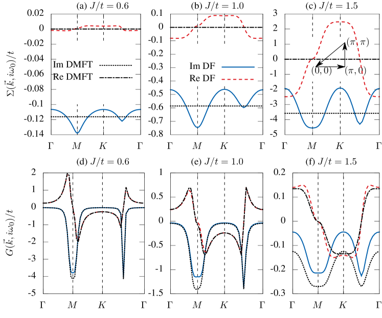
Figure 6: The momentum evolution of the self-energy function of the anti-ferromagnetic Kondo model. The inverse temperature is set as $\beta t=25$. $\Sigma(\vec{k},i\omega_{0})/t$ is shown for three different values of $J/t$ in (a), (b) and (c) respectively. The momentum dependence of $\Sigma(\vec{k},i\omega_{n})$ becomes more pronounced with the increase of $J/t$.

With the action of the dual variables,

$$S[d,d^{*}]=\sum_{\alpha}d_{\alpha}^{*}G_{0,\alpha}^{dual,-1}d_{\alpha}+V[d^{*},d],$$ (12)

one can perturbatively determine $G_{k\omega_{n},\sigma}^{dual}$ from $G_{0,k\omega_{n},\sigma}^{dual}=1/[(\Delta(i\omega_{n})-\epsilon_{k})^{-1}+g_{\omega_{n},\sigma}]$ and $V[d,d^{*}]$. In terms of the two-particle reducible vertex, the self-energy function of the dual variables can be calculated, e.g. from the first two diagrams Rubtsov et al. (2008, 2009); Li et al. (2008) in an expansion of $V[d,d^{*}]$, as

$$\Sigma^{dual}_{\alpha_{1}} = [\frac{T}{N}\sum_{2,3,4}G^{dual}_{\alpha_{3}}\gamma_{1234}(\delta_{\alpha_{2};\alpha_{3}}-\delta_{\alpha_{1};\alpha_{2}})$$ (13)

$$-\frac{T^{2}}{2N^{2}}\sum_{2,3,4}G_{\alpha_{2}}^{dual}G_{\alpha_{3}}^{dual}G_{\alpha_{4}}^{dual}\gamma_{1234}\gamma_{4321}]\times$$

$$\delta_{\alpha_{1}+\alpha_{3};\alpha_{2}+\alpha_{4}}.$$

$G_{\alpha}^{dual}$ and $\Sigma_{\alpha}^{dual}$ are related by Dyson equation $G_{\alpha}^{dual,-1}=G_{0,\alpha}^{dual,-1}-\Sigma_{\alpha}^{dual}$. Through Eq. (10), the frequency and momentum dependent Green’s function $G_{k\omega_{n},\sigma}$ can straightforwardly be calculated.

III.2 results

The most convincing way of understanding the advantage of the DF approach over the DMFT is to explicitly see the momentum dependence of the self-energy function. We show in Fig. 6 the evolution of $\Sigma(\vec{k},\pi t)/t$ as a function of $k$ along the path indicated in the middle of Fig. 6(c). These results correspond to the inverse temperature $\beta t=25$ and only the self-energies for the lowest Matsubara frequency $i\omega_{0}$ are shown here. As we know, in the DMFT local approximation, the impurity self-energy contains only the dynamic information. It is a constant function of $k$ in the 1st Brillouin Zone (BZ). In Fig. 6(a-c), they are shown as straight lines in all three plots, i.e. the DMFT self-energy has no dispersion in momentum space. In the DF approach, due to the inclusion of the non-local fluctuations, this dispersion is nicely restored. In Fig. 6, the solid blue line and the dashed red line are the corresponding imaginary and real parts of the self-energy, they both display certain dispersions, which are missing in the DMFT calculations. We find, this dispersion is much more pronounced for larger values of $J/t$, indicating that in such case the DMFT local approximation becomes less appropriate. Interesting, we notice that the momentum dispersion is always around the DMFT solution. Thus, a coarse-graining of the self-energy in momentum space would lead to a constant value that is close to the DMFT solution. In this respect, we justify the DMFT to be essentially a reasonable approximation to the problems in which electronic correlations and the delocalization of electrons competes, as in the KLM.

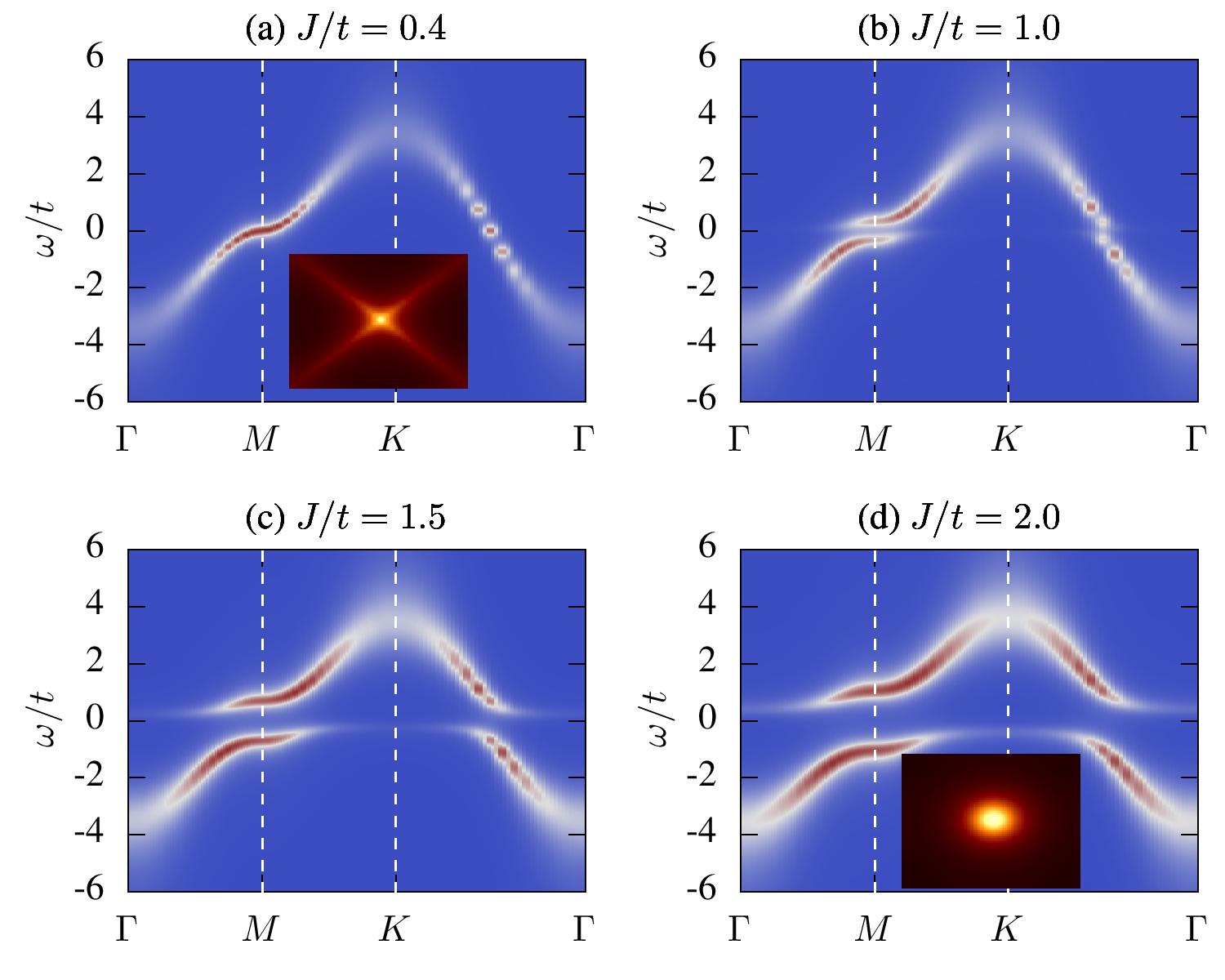
Figure 7: Single-particle spectral function of the conduction electrons at $\beta t=25$ for (a) $J/t=0.4$, (b) $J/t=1.0$, (c) $J/t=1.5$ and (d) $J/t=2.0$. The inset of (a) and (d) display the corresponding spin susceptibilities. At $J/t=1.0$ and $J/t=1.5$, the Kondo lattice model develops long-range anti-ferromagnetic order, thus spin susceptibilities are divergent and cannot be plotted.

The deviation of $\Sigma(k,i\omega_{n})$ from the DMFT solution $\Sigma(i\omega_{n})$ is more pronounced at $M$-point. With the increase of $J/t$, the real-part of $\Sigma(M,i\omega_{n})$ becomes flat around this point. As $M$-point is on the Fermi surface ($\epsilon_{M}=0$) of the non-interacting conduction electrons, the non-local corrections to $G(\vec{k},i\omega_{n})=1/(i\omega_{n}+\mu-\epsilon_{k}-\Sigma(\vec{k},i\omega_{n}))$ from $\Sigma(\vec{k},i\omega_{n})$ would be much larger here than at other values of $\vec{k}$. In Fig. 6(d-f), the single-particle Green’s function $G(\vec{k},i\omega_{n})$ are shown for the same parameters corresponding to Fig. 6(a-c). As we explained above, $G(\vec{k},i\omega_{n})$ from the DF and the DMFT calculations are mainly different at $M$-point and their difference becomes larger for larger $J/t$. For the same reason, though $\Sigma(\vec{k},i\omega_{n})$ for $\vec{k}=\Gamma$ also clearly deviates from the DMFT solution, $G(\vec{k},i\omega_{n})$ gets less affected from it, since $\epsilon_{k}$ takes the largest negative value at $\Gamma$-point. Only when the deviation becomes comparable with the half band-width, e.g. as in Fig. 6(c), $G(\Gamma,i\omega_{n})$ becomes different from the DMFT one, see Fig. 6(f).

What is more interesting is, that $\Sigma(\vec{k},i\omega_{n})$ shows an additional symmetry which cannot be described by either $\Gamma$, $M$ or $K$. In $K-\Gamma$ direction, we clearly observe another symmetry line. The real-part of $\Sigma(\vec{k},i\omega_{n})$ is anti-symmetric and the imaginary-part is symmetric with respect to this symmetry. This is exactly where the Fermi surface of the non-interacting system locates, and it is also the magnetic zone boundary for the $(\pi,\pi)$-antiferromagnetic order. Clearly, due to the inclusion of non-locality, the DF calculations capture the signature of the spin excitation. As the DMFT self-energy does not couple to any $k$-dependent collective excitation, it is not possible for the DMFT to get this additional symmetry.

Fig. 7 displays the single-particle spectral function $A(\vec{k},\omega)=-\mbox{Im}G(\vec{k},\omega)/\pi$ of the conduction electrons with four different values of $J/t$ at $\beta t=25$ in the paramagnetic phase. $A(\vec{k},\omega)$ is obtained from the corresponding single-particle Matsubara Green’s function $G(\vec{k},i\omega_{n})$ from the stochastic analytic continuation Beach . From Fig. 3 and Fig. 4, we learn that the ground state of the anti-ferromagnetic Kondo model is insulating, at any $J/t$. At high temperature, we notice that the system can be a metal with Fermi surface connecting the node $(\pm\pi/2,\pm\pi/2)$ and antinode $(0,\pm\pi),(\pm\pi,0)$. For low $J/t$, the RKKY interaction is expected to stabilize the anti-ferromagnetic long-range order. As the appearance of the additional symmetry in Fig. 6(a-c), the inclusion of the $\vec{k}$-dependent collective excitation in the DF approach is then expected to resolve some precursor effects near the magnetic transition in $A(\vec{k},\omega)$, i.e. shadow band Martin et al. (2010). Unfortunately, we did not observe any shadow band above/below the Fermi level at $\Gamma/K$. This is probably because we simply took a constant error estimation in the stochastic analytic continuation. Shadow band contains less spectral weight compared to the other bands, which might be smeared out in the analytic continuation.

Figure 8: The spin susceptibilities of the anti-ferromagnetic Kondo model at $J/t=0.5$ (upper row) and $J/t=1.0$ (lower row) for three different hole doping levels. A change from anti-ferromagnetic to ferromagnetic correlations is observed with the hole doping, however, no stable ferromagnetic phase is established for the cases studied here.

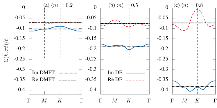
Figure 9: The momentum dependence of the self-energy function at $J/t=1.0$ with different hole concentrations. Doping the system away from half-filling, the self-energy becomes flat and the DMFT approximation becomes more justified.

In addition to inducing shadow bands, the effective RKKY interaction induced anti-ferromagnetic correlations can also drive the system to insulating. At $J/t=1.0$ (see Fig. 7(b)), the anti-ferromagnetic long-range correlation is established and splits the bands simultaneously at the Fermi level along the node and antinode direction. Fig. 7(a) and Fig. 7(b), thus, show the metal-insulator transition driven by the effective RKKY interactions and the resulting anti-ferromagnetic correlations. When the coupling of the conduction electrons and the local moments becomes larger, the Kondo effect starts to take effect. As shown in Fig. 7(c), the valence band extends to $K$ from both node and antinode. We would expect to have a large Fermi surface when we dope the system with holes. At the same time, the conduction band extends to $\Gamma$ from node and antinode. Similarly, if we dope the system with electrons, a small Fermi surface will be obtained. Though, $A(\vec{k},\omega)$ in Fig. 7(b, c, d) all contain a charge gap at the Fermi level, the mechanism for gaping is essentially different. In Fig. 7(b), the conduction electrons is decoupled with the local moments, the charge degree of freedom is gaped by the collective spin excitation induced by the effective RKKY interaction. In Fig. 7(d), the Kondo singlet forms, the conduction electron is bounded with local moments and, thus, is localized. Each site is occupied by one conduction electron anti-ferromagnetically coupled with the local magnetic moments, while the empty and doubly-occupied states at half-filling only appear virtually. The situation in Fig. 7(c) is more complicated, thus, actually more interesting. It is an anti-ferromagnetic insulator, the RKKY interaction is still playing roles, however, the additional band features at $K$ and $\Gamma$ are also apparent. Thus, the Kondo screening coexists with the anti-ferromagnetic long-range order in this phase Zhang and Yu (2000); Capponi and Assaad (2001).

The phase shown in Fig. 7(d) is termed as spin-liquid Tsunetsugu et al. (1997). The spin-liquid phase extends to $J/t=0$ in one-dimension Kondo model Fye and Scalapino (1990, 1991); Yu and White (1993). At two-dimension, the RKKY interaction favors the anti-ferromagnetic alignment of the spins between neighboring sites for small $J/t$, the ground state is an anti-ferromagnetic insulator. The spin-liquid phase is favored only at high $J/t$, where the Kondo interaction overwhelms the RKKY interaction. At high temperatures, the anti-ferromagnetic insulating states is unstable with respect to the thermal fluctuations, while the Kondo insulating states is found to be more robust. As a result, the “metal”-“anti-ferromagnetic insulator”-“Kondo insulator” transition is observed in Fig. 7 (Fig. 7(a) paramagnetic metal; Fig. 7(b, c) antiferromagnetic insulator; Fig. 7(d) Kondo insulator).

The spin-liquid phase is magnetically disordered with the corresponding spin susceptibilities being finite. In the inset of Fig. 7(d), the spin susceptibility $\chi_{s}(Q)$ is shown in the entire 1st BZ. $\chi_{s}(Q)$ peaks at $\vec{Q}=(\pi,\pi)$ and is rotationally invariant about $(\pi,\pi)$. This is similar as the spin susceptibilities in the Hubbard model with a small on-site Coulomb replusion $U$. However, we need to note that in the Hubbard model, increasing $U$ leads to the enhancement of $\chi_{s}(Q)$. While, in the Kondo model, further increase $J/t$ would suppress $\chi^{spin}(Q)$ as the Kondo singlet would have lesser overlap with the neighboring ones. Interestingly, in the paramagnetic metallic phase, e.g. see Fig. 7(a), the spin susceptibility shows a different structure. In addition to the peak at $Q=(\pi,\pi)$, $\chi_{s}(Q)$ also shows considerable amount of weight along $k_{x}=\pm k_{y}$. The different structure of the spin susceptibility signals the difference between the two paramagnetic states at low and high $J/t$ in terms of magnetic correlations, which is in line with the RKKY and Kondo interactions. In the RKKY regime, the electron spin susceptibilities are mainly contributed by the electron-hole excitations along the perfect nested Fermi surface. Due to the square shape of the Fermi surface in the 1st BZ, the majority of the momentum vectors connecting two different pieces of Fermi surface follows $k_{x}=\pm k_{y}$. While, in the Kondo regime, the Fermi surface disappear, the low energy excitation is between the top of the valence band and the bottom of the conduction band. These portions of the bands in the 1st BZ are not straight lines any more, but more extended. Thus, every combination of $k_{x},k_{y}$ is possible, which results in the rotationally invariance of the spin susceptibilities.

Now, let us move away from half-filling and study the destruction of the spin liquid phase against hole doping. When doping the system with holes, the Fermi energy moves into the valence band, the spin-liquid phase evolves into the heavy Fermi liquid state with enhanced quasiparticle mass and a large Fermi surface. Intuitive mean-field studies of the phase diagram Fazekas and Müller-Hartmann (1991) indicate that, at two-dimension, for low $J/t$ the RKKY anti-ferromagnetic phase extends to $\langle n\rangle\sim 0.58$, then it is replaced by a RKKY ferromagnetic phase. For large $J/t$, the Kondo paramagnetic phase survives even with large hole concentrations, only at very large $J/t$ the Nagaoka ferromagnetism overwhelms the Kondo paramgnetism. Similarly, the ferromagnetism at small $J/t$ in the one-dimension Kondo lattice model was also numerically studied by many different approaches, e.g. quantum Monte Carlo Troyer and Würtz (1993), density matrix renormalization group McCulloch et al. (2002), the DMFT Peters and Kawakami (2012), exact diagonalization Basylko et al. (2008), etc. The ferromagnetic phase is found to be stable at filling $\langle n\rangle<J/3t$. In addition, a ferromagnetic phase is also observed in the intermediate filling region, which entirely embeds inside the paramagnetic regime. Compared to the one-dimension case, less numerical results are known for two-dimension Kondo lattice model at away-filling case, especially for the magnetic ordering. Recently, Robert Peters et al. (2013) and Takahiro Misawa et al. (2013) etc. found a charge ordered phase at quarter-filling, which coexists with the anti-ferromagnetic phase at low temperature.

Here, we study the magnetic correlations of the KLM with the DMFT and DF approaches. Our strategy here is to calculate the spin susceptibility in the paramagnetic phase and to look for the divergence of it, which corresponds to the instability of the paramagnetic solution. From which $Q$ the spin susceptibility $\chi_{s}(Q)$ becomes divergent, we can interpret the type of the magnetic ordering that breaks the paramagnetic symmetry. Fig. 8 displays the spin susceptibilities for two values of $J/t$ and three different hole concentrations. From $(a)\rightarrow(c)$, we see the peak of the spin susceptibility at $(\pi,\pi)$ splits into four peaks and gradually moves their position from $(\pi,\pi)$ to $(0,\pm\pi)$ and $(\pm\pi,0)$. At the mean time, its amplitude is suppressed. Further increasing the hole concentration results in a continuous movement of the peaks to $Q=\Gamma$, see Fig. 8(c), which shows a tendency towards a ferromagnetic phase. We find, the susceptibility basically does not change upon increasing $J/t$ to moderate value like $J/t=1.0$ (not shown here) Only the structure gets smoother due to the same reason as for Fig. 7(a, d) (insets). However, further increasing $J/t$ and decreasing temperature $T$ will induce a divergence in $\chi_{s}(\Gamma)$, see Fig. 8(d), which possibly corresponds to the Nagaoka ferromagnetism. While, for small $J/t$, the ferromagnetic states are not really stable, no long-range order could be detected in our calculations. We further find, that the spin susceptibilities calculated from the DMFT and the DF approaches agree with each other very well, especially in the large hole doped case. Thus, we believe that the non-local fluctuation is weak in the large doping regime. This can be further understood from Fig. 9, where the momentum dependence of the self-energy functions are shown for the same doppings with $J/t=1.0$. Close to half-filling, the non-local fluctuation strongly modifies the self-energy function which induces an momentum dispersion as shown in Fig. 9(c). Increasing hole concentration, the difference between the DMFT solution and the DF solutions becomes less obvious. The DF results now become closer to the DMFT local solution, leading to the conclusion that the non-local fluctuation becomes unimportant in the hole doped case, thus, the DMFT should be a very reasonable and reliable approximation in this case.

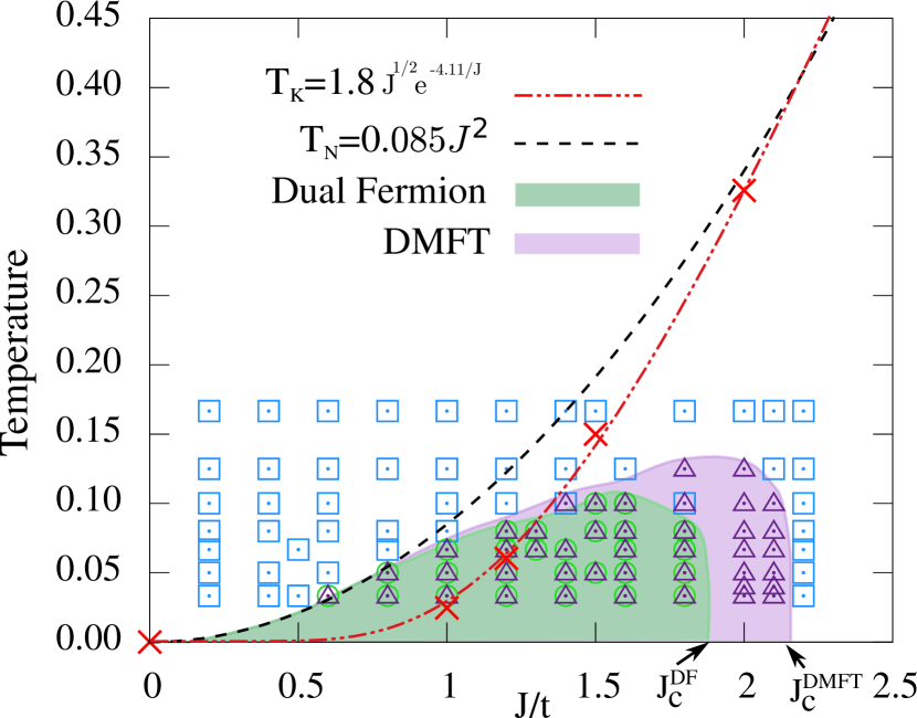
Figure 10: Doniach diagram, where the antiferromagnetic regime and the Kondo insulator regime are separated at $J_{c}$. $J_{c}$ shows a sizable non-locality dependence from the comparison of $J_{c}^{DMFT}$ and $J_{c}^{DF}$. The light green and light purple color-filled regions are determined for corresponding antiferromagnetism in the DMFT and the DF, they only serves as the guide to the eyes. The exact solutions are given as symbols (see text for more details.)

However, at half-filling, with respect to the size of the antiferromagnetic phase, the DMFT shows a strong deviation from the DF results. In Fig. 10, we summarize our results for the antiferromagnetism to the Kondo insulator transition, which is also discussed in Fig. 7, from the DMFT and the DF calculations. As stated before, by calculating the exact local two-particle vertex from the CT-HYB, we can determine the spin susceptibilities $\chi^{DMFT}_{s}(Q)$ and $\chi^{DF}_{s}(Q)$. The antiferromagnetic phase are given by the divergence of $\chi^{DMFT}_{s}(Q)$ and $\chi^{DF}_{s}(Q)$ at $Q=(\pi,\pi)$. In Fig. 10, the paramagnetic solutions are shown as blue square. In the DMFT, the antiferromagnetic phase are labeled as light-purple triangles, which clearly shows different T-J relations at large and small values of $J/t$. This highlights the competition of the RKKY and the Kondo interactions. When $J/t$ is small, the Néel temperature $T_{N}$ increases with the increase of $J/t$. $T_{N}$ can be fitted approximately as $T_{N}=0.085J^{2}$. The same $J^{2}$-dependence of $T_{N}$ is also found in our DF calculations, i.e. for smaller $J/t$, the DMFT and the DF gives essentially the same solutions. At large $J/t$, in both the DMFT and the DF calculations, we find a quick reduction of the Néel temperature, which drops to zero very rapidly at $J_{c}^{DMFT}\sim 2.15\pm 0.05$ and $J_{c}^{DF}\sim 1.85\pm 0.05$. The different values of $J_{c}$ in the DMFT and the DF calculations indicate that, the non-locality becomes more relevant at larger $J/t$ side, which seems to be unexpected. As the RKKY interaction (the effective interaction between different magnetic moments) in the smaller $J/t$ regime is non-local, while the Kondo singlet is formed locally from the magnetic impurity and the polarization of the conduction electrons, we would expect the non-local effect is more important in the RKKY regime, thus the deviation of the DMFT and the DF to be larger at smaller $J/t$. We believe this is due to the perfect nesting of the fermi surface at smaller $J/t$, compared to which the non-locality becomes less important and can be neglected. However, with the increase of $J/t$, the nesting fermi-surface is gradually lost, non-local fluctuations become visible to the system. Thus, the fermi-surface nesting suppresses the influence from the non-local fluctuations, which leads to the nice agreement of the DMFT and the DF at smaller $J/t$. And for larger $J/t$, the non-local fluctuation effect starts to play roles.

In Fig. 10, the Kondo temperature is approximately determined from the inverse of the impurity susceptibility from the DMFT, i.e. $T_{K}=C_{Z}/\chi^{imp}_{s}(T)$, at $T/t=0.01$. Following Doniach’s energy argument, we find $T_{K}$ can be fitted as $4.65Exp[-5.26/J]$. By taking into account the spin-degeneracy, as suggested by P. Coleman, we find $T_{K}$ can also be fitted approximately as $T_{K}=1.8J^{1/2}Exp[-4.11/J]$. These two fittings are nearly on top of each other for the $J/t$ values studied here. The anti-ferromagnetic phase extends to $J/t=0$ limit in Fig. 10, which partly due to the nested structure of the Fermi-surface at two-dimension. Therefore, it would be very interesting to know how the Doniach’s diagram is modified when the Fermi-surface nesting is removed, for example, by the geometric frustration in a triangular system. Li and Kirchner

IV Conclusion

In this paper, we present a detailed implementation of the dual fermion approach, in conjugation with the hybridization expansion of the continuous-time quantum Monte Carlo algorithm. The single-particle Green’s function and the two-particle reducible vertex are sampled directly in the Matsubara frequency space, with supplemented self-energy high-frequency tail. We applied our implementation to the two-dimension Kondo lattice model, where we find that the non-local fluctuations is strong at half-filling and becomes less important when the system is doped. The anti-ferromagnetic correlation induces one additional symmetry to the self-energy function, which can be nicely explained by the Néel magnetic ordering. At finite-temperature, we find a “metal”-“anti-ferromagnetic insulator”-“Kondo insulator” transition, which is resulted by the competition of the effective RKKY interaction at low $J/t$ and the Kondo effect at large $J/t$. The formation of the Kondo singlet opens the charge gap and induces additional spectra around $K$ below the Fermi level and around $\Gamma$ above the Fermi level. Correspondingly, the change of the Fermi surface shape leads to different structures in the spin susceptibilities. We confirm the Kondo effect and the anti-ferromagnetic correlations coexist at half-filling. We find the non-local fluctuations have more pronounced influence at the larger $J/t$ regime, the critical value of $J_{c}$ for the antiferromagnetism to the Kondo insulator transition is largely reduced when the non-locality is included. By doping the system, we further find that the anti-ferromagnetic correlation is destroyed and the spin susceptibility tends to peak at $Q=\Gamma$, which favors the ferromagnetic phase. However, no long-range ferromagnetic states is stabilized in our calculations for small $J/t$. In the doped case, the DMFT local approximation becomes very reliable due to the fade of the non-local fluctuations in this case.