Nonequilibrium first-order phase transition in coupled oscillator systems with inertia and noise

Shamik Gupta1, Alessandro Campa2 and Stefano Ruffo3 1Laboratoire de Physique Théorique et Modèles Statistiques (UMR CNRS 8626), Université Paris-Sud, Orsay, France
2Health and Technology Department, Istituto Superiore di Sanità, and INFN Sezione Roma1, Gruppo Collegato Sanità, Roma, Italy
3Department of Physics and Astronomy and CSDC, University of Florence, CNISM and INFN, via G. Sansone, 1 50019 Sesto Fiorentino, Italy
Abstract

We study the dynamics of a system of coupled oscillators of distributed natural frequencies, by including the features of both thermal noise, parametrized by a temperature, and inertial terms, parametrized by a moment of inertia. For a general unimodal frequency distribution, we report here the complete phase diagram of the model in the space of dimensionless moment of inertia, temperature, and width of the frequency distribution. We demonstrate that the system undergoes a nonequilibrium first-order phase transition from a synchronized phase at low parameter values to an incoherent phase at high values. We provide strong numerical evidence for the existence of both the synchronized and the incoherent phase, treating the latter analytically to obtain the corresponding linear stability threshold that bounds the first-order transition point from below. In the limit of zero noise and inertia, when the dynamics reduces to the one of the Kuramoto model, we recover the associated known continuous transition. At finite noise and inertia but in the absence of natural frequencies, the dynamics becomes that of a well-studied model of long-range interactions, the Hamiltonian mean-field model. Close to the first-order phase transition, we show that the escape time out of metastable states scales exponentially with the number of oscillators, which we explain to be stemming from the long-range nature of the interaction between the oscillators.

pacs:
05.70.Fh, 05.70.Ln, 05.45.Xt

I Introduction

Collective synchronization refers to the remarkable phenomenon of a large population of coupled oscillators spontaneously synchronizing to oscillate at a common frequency, despite each constituent having a different natural frequency. This many-body cooperative effect is observed in many physical and biological systems, pervading length and time scales of several orders of magnitude. Some examples are metabolic synchrony in yeast cell suspensions Bier:2000 , synchronized firings of cardiac pacemaker cells Winfree:1980 , flashing in unison by groups of fireflies Buck:1988 , voltage oscillations at a common frequency in an array of current-biased Josephson junctions Wiesenfeld:1998 , phase synchronization in electrical power distribution networks Filatrella:2008 ; Rohden:2012 ; Dorfler:2013 , rhythmic applause Neda:2000 , animal flocking behavior Ha:2010 ; see Ref. Strogatz:2003 for a recent survey.

A paradigmatic model to study synchronization is the Kuramoto model comprising N𝑁N phase-only oscillators of distributed natural frequencies that are globally coupled through the sine of their phase differences Kuramoto:1984 ; Strogatz:2000 . Specifically, the system involves N𝑁N interacting oscillators i=1,2,,N𝑖12𝑁i=1,2,\ldots,N. The i𝑖i-th oscillator has natural frequency ωisubscript𝜔𝑖\omega_{i}, and is characterized by its phase θisubscript𝜃𝑖\theta_{i} which is a periodic variable of period 2π2𝜋2\pi. The ωisubscript𝜔𝑖\omega_{i}’s have a common probability distribution given by g(ω)𝑔𝜔g(\omega). The phase θisubscript𝜃𝑖\theta_{i} evolves in time according to the equation

dθidt=ωi+K~Nj=1Nsin(θjθi),dsubscript𝜃𝑖d𝑡subscript𝜔𝑖~𝐾𝑁superscriptsubscript𝑗1𝑁subscript𝜃𝑗subscript𝜃𝑖\frac{\mbox{d}\theta_{i}}{\mbox{d}t}=\omega_{i}+\frac{\widetilde{K}}{N}\sum_{j=1}^{N}\sin(\theta_{j}-\theta_{i}), (1)

where K~~𝐾\widetilde{K} is the coupling constant, while the factor 1/N1𝑁1/N makes the model well behaved in the continuum limit N𝑁N\to\infty.

In this work, we study a generalization of the dynamics Eq. (1) that includes inertial terms parametrized by a moment of inertia and stochastic noise parametrized by a temperature Acebron:1998 ; Hong:1999 ; Acebron:2000 . Noise accounts for the temporal fluctuations of the natural frequencies Sakaguchi:1988 , while inertia elevates the first-order Kuramoto dynamics to second-order Ermentrout:1991 . For a general unimodal distribution of the natural frequencies, we report here the complete phase diagram of the model in the space of dimensionless moment of inertia, temperature, and width of the frequency distribution, showing that the system in the steady state may exist in either of two possible phases, namely, a synchronized phase and an unsynchronized or incoherent phase. We show that a nonequilibrium first-order transition occurs from the synchronized phase at low parameter values to the incoherent phase at high values. While strong numerical evidence is provided to support the existence of both the synchronized and the incoherent phase, only the latter could be treated analytically to obtain the corresponding linear stability threshold that bounds the first-order transition point from below. In proper limits of the dynamics, we recover the known continuous phase transitions in the Kuramoto model and in its noisy extension Sakaguchi:1988 , and an equilibrium continuous transition in a related model of long-range interactions, the Hamiltonian mean-field model Inagaki:1993 .

The Kuramoto model has been almost exclusively studied within the field of synchronization and non-linear dynamical systems. On the other hand, there has been much recent activity within the community of statistical physicists to study nonequilibrium stationary states (NESSs) and develop a general framework akin to the one due to Boltzmann and Gibbs for equilibrium that allows analysis of nonequilibrium states on a general footing Mallick:2009 . Unfortunately, there are few examples of NESSs for which one knows the probability measure of configurations exactly, so that the bulk of studies have relied on numerical simulations and approximate analysis Privman:1997 .

Our work interprets the dynamics of the Kuramoto model to be of true non-equilibrium character. Moreover, quenched disorder in the form of natural frequencies of the oscillators provides a very rich setting to study the interplay of the nonequilibrium character of the dynamics with the disorder. In this rich backdrop, we are able to characterize the nature of the NESS and ascertain under quite general conditions the whole spectrum of phase transitions.

The paper is organized as follows. In the following section, we describe the model of interest and briefly review previous studies of the model. In Sec. III, we present the complete phase diagram of the model, providing numerical simulation results in support. In Sec. IV, we present an analytical treatment of the properties of the incoherent phase, based on the Kramers equation for the single-oscillator distribution. This is followed in Sec. V by a comparison of our analytical predictions with numerical simulations. The paper ends with conclusions. Some of the technical details are relegated to the two appendices.

II The model

We now give a precise definition of the generalized dynamics that we study in this paper. In addition to phase θisubscript𝜃𝑖\theta_{i}, we associate with the i𝑖i-th oscillator another dynamical variable, namely, the angular velocity visubscript𝑣𝑖v_{i}. With a Gaussian noise force ηi(t)subscript𝜂𝑖𝑡\eta_{i}(t) and the natural frequency ωisubscript𝜔𝑖\omega_{i}, the dynamics is Acebron:1998 ; Acebron:2000

dθidt=vi,mdvidt=γvi+Krsin(ψθi)+γωi+γηi(t),formulae-sequencedsubscript𝜃𝑖d𝑡subscript𝑣𝑖𝑚dsubscript𝑣𝑖d𝑡𝛾subscript𝑣𝑖𝐾𝑟𝜓subscript𝜃𝑖𝛾subscript𝜔𝑖𝛾subscript𝜂𝑖𝑡\frac{\mbox{d}\theta_{i}}{\mbox{d}t}=v_{i},m\frac{\mbox{d}v_{i}}{\mbox{d}t}=-\gamma v_{i}+Kr\sin(\psi-\theta_{i})+\gamma\omega_{i}+\sqrt{\gamma}\eta_{i}(t), (2)

where m𝑚m is the oscillator moment of inertia, γ𝛾\gamma is the friction constant, while r𝑟r is the synchronization order parameter:

r(t)eiψ(t)j=1Neiθj(t)N.𝑟𝑡superscript𝑒𝑖𝜓𝑡superscriptsubscript𝑗1𝑁superscript𝑒𝑖subscript𝜃𝑗𝑡𝑁r(t)e^{i\psi(t)}\equiv\frac{\sum_{j=1}^{N}e^{i\theta_{j}(t)}}{N}. (3)

Here, we have

ηi(t)=0,ηi(t)ηj(t)=2Tδijδ(tt),formulae-sequencedelimited-⟨⟩subscript𝜂𝑖𝑡0delimited-⟨⟩subscript𝜂𝑖𝑡subscript𝜂𝑗superscript𝑡2𝑇subscript𝛿𝑖𝑗𝛿𝑡superscript𝑡\langle\eta_{i}(t)\rangle=0,\langle\eta_{i}(t)\eta_{j}(t^{\prime})\rangle=2T\delta_{ij}\delta(t-t^{\prime}), (4)

with temperature T𝑇T in units of the Boltzmann constant. We consider a unimodal g(ω)𝑔𝜔g(\omega) (that is, symmetric about mean ω~~𝜔\widetilde{\omega}, and decreases to zero with increasing |ωω~|𝜔~𝜔|\omega-\widetilde{\omega}|), and denote its width by σ𝜎\sigma. In the absence of inertia, the dynamics with the redefinition K/γ=K~𝐾𝛾~𝐾K/\gamma=\widetilde{K} reduces at T=0𝑇0T=0 to that of the Kuramoto model Kuramoto:1984 ; Strogatz:2000 and at T0𝑇0T\neq 0 to that of its extension studied by Sakaguchi in Ref. Sakaguchi:1988 .

The dynamics Eq. (2) also describes motion of particles with an XY𝑋𝑌XY-interaction on a unit circle, with θi,visubscript𝜃𝑖subscript𝑣𝑖\theta_{i},v_{i} and γωi𝛾subscript𝜔𝑖\gamma\omega_{i} being respectively the angular coordinate, velocity and external torque. In the absence of ωisubscript𝜔𝑖\omega_{i}’s, Eq. (2) for γ=0𝛾0\gamma=0 is the microcanonical dynamics of the Hamiltonian mean-field model Inagaki:1993 , a prototype of long-range interacting systems Campa:2009 . In this case, the equations of motion are the Hamilton equations associated with the Hamiltonian

H=i=1Npi22m+K2Ni,j=1N[1cos(θiθj)],𝐻superscriptsubscript𝑖1𝑁superscriptsubscript𝑝𝑖22𝑚𝐾2𝑁superscriptsubscript𝑖𝑗1𝑁delimited-[]1subscript𝜃𝑖subscript𝜃𝑗H=\sum_{i=1}^{N}\frac{p_{i}^{2}}{2m}+\frac{K}{2N}\sum_{i,j=1}^{N}\Big{[}1-\cos(\theta_{i}-\theta_{j})\Big{]}, (5)

with pi=mvisubscript𝑝𝑖𝑚subscript𝑣𝑖p_{i}=mv_{i} the momentum of the i𝑖i-th particle. The dynamics of this system is microcanonical, conserving energy and total momentum. With no ωisubscript𝜔𝑖\omega_{i}’s, but γ0𝛾0\gamma\neq 0, the dynamics of the resulting Brownian mean-field (BMF) model is canonical, mimicking the interaction of the HMF system with a heat bath Chavanis:2013 .

The dynamics Eq. (2) is invariant under θiθi+ω~t,vivi+ω~,ωiωi+ω~formulae-sequencesubscript𝜃𝑖subscript𝜃𝑖~𝜔𝑡formulae-sequencesubscript𝑣𝑖subscript𝑣𝑖~𝜔subscript𝜔𝑖subscript𝜔𝑖~𝜔\theta_{i}\to\theta_{i}+\widetilde{\omega}t,v_{i}\to v_{i}+\widetilde{\omega},\omega_{i}\to\omega_{i}+\widetilde{\omega}, and the effect of σ𝜎\sigma may be made explicit by replacing ωisubscript𝜔𝑖\omega_{i} in the second equation with σωi𝜎subscript𝜔𝑖\sigma\omega_{i}. We thus consider from now on the dynamics Eq. (2) with the substitution ωiσωisubscript𝜔𝑖𝜎subscript𝜔𝑖\omega_{i}\rightarrow\sigma\omega_{i}. In the resulting model, we take g(ω)𝑔𝜔g(\omega) to have zero mean and unit width, without loss of generality.

For m0𝑚0m\neq 0, using dimensionless variables

t¯tK/m,¯𝑡𝑡𝐾𝑚\displaystyle\overline{t}\equiv t\sqrt{K/m}, (6)
v¯ivim/K,subscript¯𝑣𝑖subscript𝑣𝑖𝑚𝐾\displaystyle\overline{v}_{i}\equiv v_{i}\sqrt{m/K}, (7)
1/m¯γ/Km,1¯𝑚𝛾𝐾𝑚\displaystyle 1/\sqrt{\overline{m}}\equiv\gamma/\sqrt{Km}, (8)
σ¯γσ/K,¯𝜎𝛾𝜎𝐾\displaystyle\overline{\sigma}\equiv\gamma\sigma/K, (9)
T¯T/K,¯𝑇𝑇𝐾\displaystyle\overline{T}\equiv T/K, (10)
η¯i(t¯)ηi(t)γ/K,subscript¯𝜂𝑖¯𝑡subscript𝜂𝑖𝑡𝛾𝐾\displaystyle\overline{\eta}_{i}(\overline{t})\equiv\eta_{i}(t)\sqrt{\gamma}/K, (11)

the dynamics becomes

dθidt¯=v¯i,dv¯idt¯=1m¯v¯i+rsin(ψθi)+σ¯ωi+η¯i(t¯),formulae-sequencedsubscript𝜃𝑖d¯𝑡subscript¯𝑣𝑖dsubscript¯𝑣𝑖d¯𝑡1¯𝑚subscript¯𝑣𝑖𝑟𝜓subscript𝜃𝑖¯𝜎subscript𝜔𝑖subscript¯𝜂𝑖¯𝑡\displaystyle\frac{\mbox{d}\theta_{i}}{\mbox{d}\overline{t}}=\overline{v}_{i},\frac{\mbox{d}\overline{v}_{i}}{\mbox{d}\overline{t}}=-\frac{1}{\sqrt{\overline{m}}}\overline{v}_{i}+r\sin(\psi-\theta_{i})+\overline{\sigma}\omega_{i}+\overline{\eta}_{i}(\overline{t}),
(12)

where

η¯i(t¯)η¯j(t¯)=2T¯m¯δijδ(t¯t¯).delimited-⟨⟩subscript¯𝜂𝑖¯𝑡subscript¯𝜂𝑗superscript¯𝑡2¯𝑇¯𝑚subscript𝛿𝑖𝑗𝛿¯𝑡superscript¯𝑡\langle\overline{\eta}_{i}(\overline{t})\overline{\eta}_{j}(\overline{t}^{\prime})\rangle=2\frac{\overline{T}}{\sqrt{\overline{m}}}\delta_{ij}\delta(\overline{t}-\overline{t}^{\prime}). (13)

For m=0𝑚0m=0, using dimensionless time t¯t(K/γ)¯𝑡𝑡𝐾𝛾\overline{t}\equiv t(K/\gamma), the dynamics becomes the overdamped motion

dθidt¯=rsin(ψθi)+σ¯ωi+η¯i(t¯),dsubscript𝜃𝑖d¯𝑡𝑟𝜓subscript𝜃𝑖¯𝜎subscript𝜔𝑖subscript¯𝜂𝑖¯𝑡\frac{\mbox{d}\theta_{i}}{\mbox{d}\overline{t}}=r\sin(\psi-\theta_{i})+\overline{\sigma}\omega_{i}+\overline{\eta}_{i}(\overline{t}), (14)

where

η¯i(t¯)η¯j(t¯)=2T¯δijδ(t¯t¯).delimited-⟨⟩subscript¯𝜂𝑖¯𝑡subscript¯𝜂𝑗superscript¯𝑡2¯𝑇subscript𝛿𝑖𝑗𝛿¯𝑡superscript¯𝑡\langle\overline{\eta}_{i}(\overline{t})\overline{\eta}_{j}(\overline{t}^{\prime})\rangle=2\overline{T}\delta_{ij}\delta(\overline{t}-\overline{t}^{\prime}). (15)

From now on, we will consider in place of dynamics Eq. (2) the reduced dynamics Eq. (12) [that reduces for m=0𝑚0m=0 to the overdamped dynamics Eq. (14)] involving three dimensionless parameters, m¯,T¯,σ¯¯𝑚¯𝑇¯𝜎\overline{m},\overline{T},\overline{\sigma}; we will drop overbars for simplicity of notation. With σ=0𝜎0\sigma=0 (i.e. g(ω)=δ(ω)𝑔𝜔𝛿𝜔g(\omega)=\delta(\omega) Acebron:1998 ,Acebron:2000 ), the resulting BMF dynamics has an equilibrium stationary state Chavanis:2013 . For other g(ω)𝑔𝜔g(\omega), the dynamics Eq. (12) violates detailed balance due to the external driving by the set of torques {γωi}𝛾subscript𝜔𝑖\{\gamma\omega_{i}\}, yielding a NESS. We demonstrate this in Appendix A.

Several stationary state aspects of the dynamics Eq. (12) in the continuum limit N𝑁N\to\infty are known. For the Kuramoto dynamics (m=T=0𝑚𝑇0m=T=0), the system exhibits a continuous transition from a low-σ𝜎\sigma synchronized [rst=r(t)0subscript𝑟st𝑟𝑡0r_{\rm st}=r(t\to\infty)\neq 0] to a high-σ𝜎\sigma incoherent (rst=0subscript𝑟st0r_{\rm st}=0) phase across the critical point Kuramoto:1984

σc(m=0,T=0)=πg(0)2;subscript𝜎𝑐formulae-sequence𝑚0𝑇0𝜋𝑔02\sigma_{c}(m=0,T=0)=\frac{\pi g(0)}{2}; (16)

extending to T0𝑇0T\neq 0, the point becomes a second-order critical line σc(m=0,T)subscript𝜎𝑐𝑚0𝑇\sigma_{c}(m=0,T) on the (T,σ)𝑇𝜎(T,\sigma)-plane, given, on using the results of Sakaguchi in Ref. Sakaguchi:1988 , by solving

2=Tg(ω)dωT2+ω2σc2(m=0,T).2superscriptsubscript𝑇𝑔𝜔d𝜔superscript𝑇2superscript𝜔2subscriptsuperscript𝜎2𝑐𝑚0𝑇2=\int_{-\infty}^{\infty}\frac{Tg(\omega)\mbox{d}\omega}{T^{2}+\omega^{2}\sigma^{2}_{c}(m=0,T)}. (17)

For the BMF dynamics (σ=0;m,T0formulae-sequence𝜎0𝑚𝑇0\sigma=0;~{}m,T\neq 0), the synchronization transition is again continuous, occurring at the critical temperature given by Chavanis:2013

Tc=12.subscript𝑇𝑐12T_{c}=\frac{1}{2}. (18)

Although there have been some numerical studies of the full dynamics for non-zero m,T,σ𝑚𝑇𝜎m,T,\sigma Tanaka:1997 ; Acebron:1998 ; Acebron:2000 , the complete synchronization phase diagram for a general unimodal g(ω)𝑔𝜔g(\omega) has not been addressed before, a question we take up and answer in this paper. In the next section, we describe the complete phase diagram that emerges out of our analysis.
Refer to caption
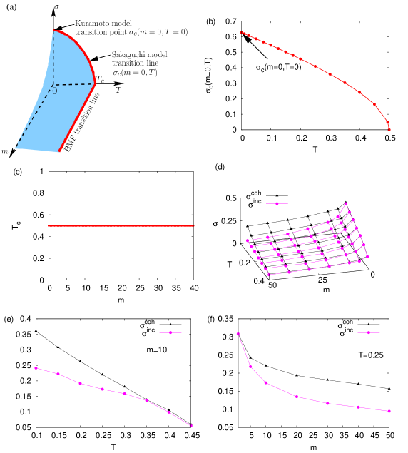
Figure 1: (Color online) (a) Schematic phase diagram of model Eq. (12) in terms of dimensionless moment of inertia m𝑚m, temperature T𝑇T, and width σ𝜎\sigma of the frequency distribution: the shaded blue surface is a first-order transition surface, the thick red lines are second-order critical lines. The system is synchronized inside the region bounded by the surface, and is incoherent outside. The limits (the Kuramoto model, the Sakaguchi model and the BMF model) in which known transitions are obtained are labeled. (b) The known transition line for the Sakaguchi model, given by Eq. (17), showing also the Kuramoto model transition point, Eq. (16), for a Gaussian g(ω)𝑔𝜔g(\omega) with zero mean and unit width width . (c) The known transition line for the BMF model, given by Eq. (18). The shaded blue surface in (a) is bounded from above and below by the dynamical stability thresholds σcoh(m,T)superscript𝜎coh𝑚𝑇\sigma^{\rm coh}(m,T) and σinc(m,T)superscript𝜎inc𝑚𝑇\sigma^{\rm inc}(m,T) of the synchronized and the incoherent phase respectively. These thresholds may be estimated in N𝑁N-body simulations from hysteresis plots (see Fig. 2 for an example); Panel (d) shows the surfaces σcoh(m,T)superscript𝜎coh𝑚𝑇\sigma^{\rm coh}(m,T) and σinc(m,T)superscript𝜎inc𝑚𝑇\sigma^{\rm inc}(m,T) obtained from N𝑁N-body simulations with N=500𝑁500N=500 for a Gaussian g(ω)𝑔𝜔g(\omega) with zero mean and unit width, with cuts of the three-dimensional plot at m=10𝑚10m=10 shown in panel (e) and at T=0.25𝑇0.25T=0.25 shown in panel (f).
Refer to caption
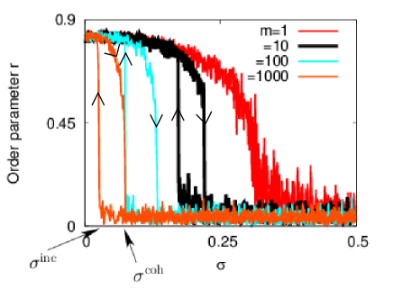
Figure 2: (Color online) r𝑟r vs. adiabatically tuned σ𝜎\sigma for different m𝑚m values at T=0.25<Tc=1/2𝑇0.25subscript𝑇𝑐12T=0.25<T_{c}=1/2, showing also the stability thresholds, σinc(m,T)superscript𝜎inc𝑚𝑇\sigma^{\rm inc}(m,T) and σcoh(m,T)superscript𝜎coh𝑚𝑇\sigma^{\rm coh}(m,T), for m=1000𝑚1000m=1000. For a given m𝑚m, the branch of the plot to the right (left) marked with an arrowhead pointing down (up) corresponds to σ𝜎\sigma increasing (decreasing); for m=1𝑚1m=1, the two branches almost overlap. The data are obtained in N𝑁N-body simulations with N=500𝑁500N=500 for a Gaussian g(ω)𝑔𝜔g(\omega) with zero mean and unit width.
Refer to caption
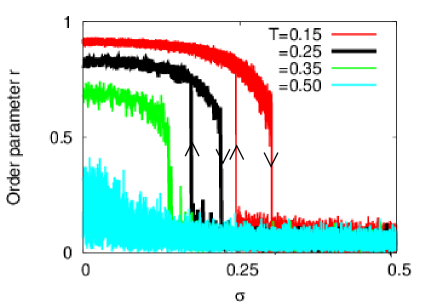
Figure 3: (Color online) r𝑟r vs. adiabatically tuned σ𝜎\sigma for different temperatures TTc=1/2𝑇subscript𝑇𝑐12T\leq T_{c}=1/2 at a fixed moment of inertia m=10𝑚10m=10. For a given T𝑇T, the branch of the plot to the right (left) marked with an arrowhead pointing down (up) corresponds to σ𝜎\sigma increasing (decreasing); for T0.35𝑇0.35T\geq 0.35, the two branches almost overlap. The data are obtained in N𝑁N-body simulations with N=500𝑁500N=500 for a Gaussian g(ω)𝑔𝜔g(\omega) with zero mean and unit width. Similar disappearance of the hysteresis loop with increase of T𝑇T was reported in Ref. Hong:1999 .

III Phase diagram

The complete phase diagram is shown schematically in Fig. 1(a), where the thick red second-order critical lines stand for the continuous transitions mentioned above. For non-zero m,T,σ𝑚𝑇𝜎m,T,\sigma, the synchronization transition becomes first-order, occurring across the shaded blue transition surface; this surface is bounded by the second-order critical lines on the (T,σ)𝑇𝜎(T,\sigma) and (m,T)𝑚𝑇(m,T) planes, and by a first-order transition line on the (m,σ)𝑚𝜎(m,\sigma)-plane.

The phase diagram in Fig. 1(a) is a generalization of the one for typical fluids where a first-order transition line ends in a critical point, while we have here a first-order transition surface ending in critical lines. All transitions for σ0𝜎0\sigma\neq 0 are in NESS, and we interpret them to be of dynamical origin, accounted for by stability considerations of stationary solutions of equations describing evolution of phase-space distribution. Showing that the phases extremize a free-energy-like quantity (e.g., a large deviation functional Touchette:2009 ) in NESS is a daunting task in the absence of a general framework akin to that for equilibrium Derrida:2005 . For σ=0𝜎0\sigma=0, the different phases actually minimize the equilibrium free energy Campa:2009 .
Refer to caption
Refer to caption
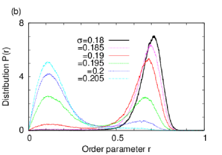
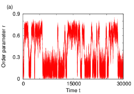
Figure 4: (Color online) For m=20,T=0.25formulae-sequence𝑚20𝑇0.25m=20,T=0.25, and a Gaussian g(ω)𝑔𝜔g(\omega) with zero mean and unit width, (a) shows at σ=0.195𝜎0.195\sigma=0.195, the numerically estimated first-order phase transition point, r𝑟r vs. time in the stationary state, while (b) shows the distribution P(r)𝑃𝑟P(r) at several σ𝜎\sigma’s around 0.1950.1950.195. The data are obtained in N𝑁N-body simulations with N=100𝑁100N=100.

To confirm the first-order transition, we performed N𝑁N-body simulations involving integrations of Eq. (12) for a representative g(ω)𝑔𝜔g(\omega), i.e., a Gaussian. Details of the simulation procedure are given in the Appendix B. For given m𝑚m and T𝑇T and an initial state with oscillators at θ=0𝜃0\theta=0 and angular velocities sampled from a Gaussian distribution with zero mean and width Tproportional-toabsent𝑇\propto T, we let the system equilibrate at σ=0𝜎0\sigma=0. We then tune σ𝜎\sigma adiabatically to high values and back in a cycle. Figure 2 shows the behavior of the synchronization order parameter r𝑟r for several m𝑚m’s at a fixed T𝑇T less than the BMF transition point Tc=1/2subscript𝑇𝑐12T_{c}=1/2, illustrating sharp jumps and hysteresis behavior expected of a first-order transition. With decrease of m𝑚m, the jump in r𝑟r becomes less sharp and the hysteresis loop area decreases, both consistent with the transition becoming second-order-like as m𝑚m decreases, see Fig. 1. For m=1000𝑚1000m=1000, Fig. 2 shows σinc(m,T)superscript𝜎inc𝑚𝑇\sigma^{\rm inc}(m,T) and σcoh(m,T)superscript𝜎coh𝑚𝑇\sigma^{\rm coh}(m,T), the stability thresholds for the incoherent and the synchronized phase, respectively; the phase transition point σc(m,T)subscript𝜎𝑐𝑚𝑇\sigma_{c}(m,T) lies in between the two thresholds (see Fig. 1(d)). Figure 2 shows that the thresholds decrease and approach zero with the increase of m𝑚m; it also suggests, together with Fig. 3, that σincsuperscript𝜎inc\sigma^{\rm inc} and σcohsuperscript𝜎coh\sigma^{\rm coh} coincide both on the second order critical lines and as m𝑚m\to\infty at a fixed T𝑇T.

For given m𝑚m and T𝑇T and σ𝜎\sigma between σinc(m,T)superscript𝜎inc𝑚𝑇\sigma^{\rm inc}(m,T) and σcoh(m,T)superscript𝜎coh𝑚𝑇\sigma^{\rm coh}(m,T), r𝑟r versus time in the stationary state shows bistability, with the system switching back and forth between incoherent and synchronized states [Fig. 4(a)]. To have not-too-large switching times, these simulations have been performed with a relatively small number of oscillators, N=100𝑁100N=100, causing large fluctuations in the order parameter r𝑟r. Therefore, in Fig. 4(a) the synchronized and the unsynchronized state are characterized by values of r𝑟r fluctuating above and below 0.40.40.4, respectively; however, this does allow for a clear visualization of the switches. The distribution P(r)𝑃𝑟P(r) in Fig. 4(b) is bimodal with a peak around r0𝑟0r\approx 0 or r>0𝑟0r>0 as σ𝜎\sigma varies between σincsuperscript𝜎inc\sigma^{\rm inc} and σcohsuperscript𝜎coh\sigma^{\rm coh}, consistent with the transition being first-order. Indeed, a first-order transition point is characterized by two equally likely values of the order parameter, while at a second-order phase transition point, the order parameter has its value equal to zero Goldenfeld:1992 .

IV Analytical treatment

We now turn to an analytical treatment of the first-order transition. In the continuum limit N𝑁N\to\infty, the dynamics Eq. (12) is described by the single-oscillator distribution f(θ,v,ω,t)𝑓𝜃𝑣𝜔𝑡f(\theta,v,\omega,t) which gives at time t𝑡t and for each ω𝜔\omega the fraction of oscillators with phase θ𝜃\theta and angular velocity v𝑣v. The distribution is 2π2𝜋2\pi-periodic in θ𝜃\theta, and obeys the normalization 02πdθdvf(θ,v,ω,t)=1superscriptsubscript02𝜋d𝜃superscriptsubscriptd𝑣𝑓𝜃𝑣𝜔𝑡1\int_{0}^{2\pi}\mbox{d}\theta\int_{-\infty}^{\infty}\mbox{d}vf(\theta,v,\omega,t)=1, while evolving following the Kramers equation Acebron:2000

ft=vfθ+v(vmσωrsin(ψθ))f+Tm2fv2,𝑓𝑡𝑣𝑓𝜃𝑣𝑣𝑚𝜎𝜔𝑟𝜓𝜃𝑓𝑇𝑚superscript2𝑓superscript𝑣2\frac{\partial f}{\partial t}=-v\frac{\partial f}{\partial\theta}+\frac{\partial}{\partial v}\Big{(}\frac{v}{\sqrt{m}}-\sigma\omega-r\sin(\psi-\theta)\Big{)}f+\frac{T}{\sqrt{m}}\frac{\partial^{2}f}{\partial v^{2}}, (19)

where reiψ=dθdvdωg(ω)eiθf(θ,v,ω,t)𝑟superscript𝑒𝑖𝜓d𝜃d𝑣d𝜔𝑔𝜔superscript𝑒𝑖𝜃𝑓𝜃𝑣𝜔𝑡re^{i\psi}=\int\mbox{d}\theta\mbox{d}v\mbox{d}\omega~{}g(\omega)e^{i\theta}f(\theta,v,\omega,t). We now give the derivation of Eq. (19), followed by a discussion of its stationary solution corresponding to the incoherent phase.

IV.1 The Kramers equation for the single-oscillator distribution: Incoherent stationary state

Here, we start with deriving the Bogoliubov-Born-Green-Kirkwood-Yvon (BBGKY) hierarchy equations for the dynamics Eq. (12) for any number of oscillators N𝑁N, and, from there, by considering the limit N𝑁N\to\infty, obtain the Kramers Eq. (19). For simplicity, we first discuss the derivation of the BBGKY equations for the case of a bimodal g(ω)𝑔𝜔g(\omega), and then generalize it to a general g(ω)𝑔𝜔g(\omega).

Consider a given realization of g(ω)𝑔𝜔g(\omega), in which there are N1subscript𝑁1N_{1} oscillators with frequencies ω1subscript𝜔1\omega_{1}, and N2subscript𝑁2N_{2} oscillators with frequencies ω2subscript𝜔2\omega_{2}, where N1+N2=Nsubscript𝑁1subscript𝑁2𝑁N_{1}+N_{2}=N. We then define the N𝑁N-oscillator distribution function fN(θ1,v1,,θN1,vN1,θN1+1,vN1+1,,θN,vN,t)subscript𝑓𝑁subscript𝜃1subscript𝑣1subscript𝜃subscript𝑁1subscript𝑣subscript𝑁1subscript𝜃subscript𝑁11subscript𝑣subscript𝑁11subscript𝜃𝑁subscript𝑣𝑁𝑡f_{N}(\theta_{1},v_{1},\dots,\theta_{N_{1}},v_{N_{1}},\theta_{N_{1}+1},v_{N_{1}+1},\dots,\theta_{N},v_{N},t) as the probability density at time t𝑡t to observe the system around the values {θi,vi}1iNsubscriptsubscript𝜃𝑖subscript𝑣𝑖1𝑖𝑁\{\theta_{i},v_{i}\}_{1\leq i\leq N}. In the following, we use the shorthand notations zi(θi,vi)subscript𝑧𝑖subscript𝜃𝑖subscript𝑣𝑖z_{i}\equiv(\theta_{i},v_{i}) and 𝐳=(z1,z2,,zN)𝐳subscript𝑧1subscript𝑧2subscript𝑧𝑁\mathbf{z}=(z_{1},z_{2},\dots,z_{N}). Note that fNsubscript𝑓𝑁f_{N} satisfies the normalization (i=1Ndzi)fN(𝐳,t)=1superscriptsubscriptproduct𝑖1𝑁dsubscript𝑧𝑖subscript𝑓𝑁𝐳𝑡1\int\Big{(}\prod_{i=1}^{N}\mbox{d}z_{i}\Big{)}f_{N}(\mathbf{z},t)=1. We assume that

  1. 1.

    fNsubscript𝑓𝑁f_{N} is symmetric with respect to permutations of dynamical variables within the group of oscillators with the same frequency, and

  2. 2.

    fNsubscript𝑓𝑁f_{N}, together with the derivatives fN/viisubscript𝑓𝑁subscript𝑣𝑖for-all𝑖\partial f_{N}/\partial v_{i}~{}\forall~{}i, vanish on the boundaries of the phase space.

The evolution of fNsubscript𝑓𝑁f_{N} follows the Fokker-Planck equation which may be straightforwardly derived from the equations of motion Eq. (12):

fNt=i=1N[vifNθi1m(vifN)vi]subscript𝑓𝑁𝑡superscriptsubscript𝑖1𝑁delimited-[]subscript𝑣𝑖subscript𝑓𝑁subscript𝜃𝑖1𝑚subscript𝑣𝑖subscript𝑓𝑁subscript𝑣𝑖\displaystyle\frac{\partial f_{N}}{\partial t}=-\sum_{i=1}^{N}\Big{[}v_{i}\frac{\partial f_{N}}{\partial\theta_{i}}-\frac{1}{\sqrt{m}}\frac{\partial(v_{i}f_{N})}{\partial v_{i}}\Big{]}
σj=1N(ΩT)jfNvj+Tmi=1N2fNvi2𝜎superscriptsubscript𝑗1𝑁subscriptsuperscriptΩ𝑇𝑗subscript𝑓𝑁subscript𝑣𝑗𝑇𝑚superscriptsubscript𝑖1𝑁superscript2subscript𝑓𝑁superscriptsubscript𝑣𝑖2\displaystyle-\sigma\sum_{j=1}^{N}\Big{(}\Omega^{T}\Big{)}_{j}\frac{\partial f_{N}}{\partial v_{j}}+\frac{T}{\sqrt{m}}\sum_{i=1}^{N}\frac{\partial^{2}f_{N}}{\partial v_{i}^{2}}
12Ni,j=1Nsin(θjθi)[fNvifNvj],12𝑁superscriptsubscript𝑖𝑗1𝑁subscript𝜃𝑗subscript𝜃𝑖delimited-[]subscript𝑓𝑁subscript𝑣𝑖subscript𝑓𝑁subscript𝑣𝑗\displaystyle-\frac{1}{2N}\sum_{i,j=1}^{N}\sin(\theta_{j}-\theta_{i})\Big{[}\frac{\partial f_{N}}{\partial v_{i}}-\frac{\partial f_{N}}{\partial v_{j}}\Big{]}, (20)

where we have defined the N×1𝑁1N\times 1 column vector ΩΩ\Omega whose first N1subscript𝑁1N_{1} entries equal ω1subscript𝜔1\omega_{1} and the following N2subscript𝑁2N_{2} entries equal ω2subscript𝜔2\omega_{2}, and where the superscript T𝑇T denotes matrix transpose operation: ΩT[ω1ω1ω1ω2ω2]superscriptΩ𝑇delimited-[]subscript𝜔1subscript𝜔1subscript𝜔1subscript𝜔2subscript𝜔2\Omega^{T}\equiv\left[\omega_{1}~{}\omega_{1}\dots~{}\omega_{1}~{}\omega_{2}\dots~{}\omega_{2}\right].

To proceed, we follow standard procedure Huang:1987 , and define the reduced distribution function fs1,s2subscript𝑓subscript𝑠1subscript𝑠2f_{s_{1},s_{2}}, with s1=0,1,2,,N1subscript𝑠1012subscript𝑁1s_{1}=0,1,2,\dots,N_{1} and s2=0,1,2,,N2subscript𝑠2012subscript𝑁2s_{2}=0,1,2,\dots,N_{2}, as

fs1,s2(z1,z2,,zs1,zN1+1,,zN1+s2,t)subscript𝑓subscript𝑠1subscript𝑠2subscript𝑧1subscript𝑧2subscript𝑧subscript𝑠1subscript𝑧subscript𝑁11subscript𝑧subscript𝑁1subscript𝑠2𝑡\displaystyle f_{s_{1},s_{2}}(z_{1},z_{2},\dots,z_{s_{1}},z_{N_{1}+1},\dots,z_{N_{1}+s_{2}},t)
=N1!(N1s1)!N1s1N2!(N2s2)!N2s2absentsubscript𝑁1subscript𝑁1subscript𝑠1superscriptsubscript𝑁1subscript𝑠1subscript𝑁2subscript𝑁2subscript𝑠2superscriptsubscript𝑁2subscript𝑠2\displaystyle=\frac{N_{1}!}{(N_{1}-s_{1})!N_{1}^{s_{1}}}\frac{N_{2}!}{(N_{2}-s_{2})!N_{2}^{s_{2}}}
dzs1+1dzN1dzN1+s2+1dzNfN(z,t).dsubscript𝑧subscript𝑠11dsubscript𝑧subscript𝑁1dsubscript𝑧subscript𝑁1subscript𝑠21dsubscript𝑧𝑁subscript𝑓𝑁𝑧𝑡\displaystyle\int\mbox{d}z_{s_{1}+1}\dots\mbox{d}z_{N_{1}}\mbox{d}z_{N_{1}+s_{2}+1}\dots\mbox{d}z_{N}f_{N}(z,t). (21)

Note that the following normalizations hold for the single-oscillator distribution functions: dz1f1,0(z1,t)=1dsubscript𝑧1subscript𝑓10subscript𝑧1𝑡1\int\mbox{d}z_{1}f_{1,0}(z_{1},t)=1, and dzN1+1f0,1(zN1+1,t)=1dsubscript𝑧subscript𝑁11subscript𝑓01subscript𝑧subscript𝑁11𝑡1\int\mbox{d}z_{N_{1}+1}f_{0,1}(z_{N_{1}+1},t)=1.

Using Eq. (20) in Eq. (21) and simplifying, we get the BBGKY hierarchy equations for oscillators with frequencies ω1subscript𝜔1\omega_{1} as

fs,0t+i=1s[vifs,0θi1mvi(vifs,0)]+σi=1sω1fs,0visubscript𝑓𝑠0𝑡superscriptsubscript𝑖1𝑠delimited-[]subscript𝑣𝑖subscript𝑓𝑠0subscript𝜃𝑖1𝑚subscript𝑣𝑖subscript𝑣𝑖subscript𝑓𝑠0𝜎superscriptsubscript𝑖1𝑠subscript𝜔1subscript𝑓𝑠0subscript𝑣𝑖\displaystyle\frac{\partial f_{s,0}}{\partial t}+\sum_{i=1}^{s}\Big{[}\frac{v_{i}\partial f_{s,0}}{\partial\theta_{i}}-\frac{1}{\sqrt{m}}\frac{\partial}{\partial v_{i}}(v_{i}f_{s,0})\Big{]}+\sigma\sum_{i=1}^{s}\omega_{1}\frac{\partial f_{s,0}}{\partial v_{i}}
Tmi=1s2fs,0vi2=12Ni,j=1ssin(θjθi)[fs,0vifs,0vj]𝑇𝑚superscriptsubscript𝑖1𝑠superscript2subscript𝑓𝑠0superscriptsubscript𝑣𝑖212𝑁superscriptsubscript𝑖𝑗1𝑠subscript𝜃𝑗subscript𝜃𝑖delimited-[]subscript𝑓𝑠0subscript𝑣𝑖subscript𝑓𝑠0subscript𝑣𝑗\displaystyle-\frac{T}{\sqrt{m}}\sum_{i=1}^{s}\frac{\partial^{2}f_{s,0}}{\partial v_{i}^{2}}=-\frac{1}{2N}\sum_{i,j=1}^{s}\sin(\theta_{j}-\theta_{i})\Big{[}\frac{\partial f_{s,0}}{\partial v_{i}}-\frac{\partial f_{s,0}}{\partial v_{j}}\Big{]}
N1Ni=1sdzs+1sin(θs+1θi)fs+1,0visubscript𝑁1𝑁superscriptsubscript𝑖1𝑠dsubscript𝑧𝑠1subscript𝜃𝑠1subscript𝜃𝑖subscript𝑓𝑠10subscript𝑣𝑖\displaystyle-\frac{N_{1}}{N}\sum_{i=1}^{s}\int\mbox{d}z_{s+1}\sin(\theta_{s+1}-\theta_{i})\frac{\partial f_{s+1,0}}{\partial v_{i}}
N2NdzN1+1i=1ssin(θN1+1θi)fs,1vi,subscript𝑁2𝑁dsubscript𝑧subscript𝑁11superscriptsubscript𝑖1𝑠subscript𝜃subscript𝑁11subscript𝜃𝑖subscript𝑓𝑠1subscript𝑣𝑖\displaystyle-\frac{N_{2}}{N}\int\mbox{d}z_{N_{1}+1}\sum_{i=1}^{s}\sin(\theta_{N_{1}+1}-\theta_{i})\frac{\partial f_{s,1}}{\partial v_{i}}, (22)

and similar equations for f0,ssubscript𝑓0𝑠f_{0,s} for oscillators of frequencies ω2subscript𝜔2\omega_{2}. The first equations of the hierarchy are

f1,0(θ,v,t)t+vf1,0(θ,v,t)θ1mv(vf1,0(θ,v,t))subscript𝑓10𝜃𝑣𝑡𝑡𝑣subscript𝑓10𝜃𝑣𝑡𝜃1𝑚𝑣𝑣subscript𝑓10𝜃𝑣𝑡\displaystyle\frac{\partial f_{1,0}(\theta,v,t)}{\partial t}+\frac{v\partial f_{1,0}(\theta,v,t)}{\partial\theta}-\frac{1}{\sqrt{m}}\frac{\partial}{\partial v}(vf_{1,0}(\theta,v,t))
+σω1f1,0(θ,v,t)vTm2f1,0(θ,v,t)v2𝜎subscript𝜔1subscript𝑓10𝜃𝑣𝑡𝑣𝑇𝑚superscript2subscript𝑓10𝜃𝑣𝑡superscript𝑣2\displaystyle+\sigma\omega_{1}\frac{\partial f_{1,0}(\theta,v,t)}{\partial v}-\frac{T}{\sqrt{m}}\frac{\partial^{2}f_{1,0}(\theta,v,t)}{\partial v^{2}}
=N1Ndθdvsin(θθ)f2,0(θ,v,θ,v,t)vabsentsubscript𝑁1𝑁dsuperscript𝜃dsuperscript𝑣superscript𝜃𝜃subscript𝑓20𝜃𝑣superscript𝜃superscript𝑣𝑡𝑣\displaystyle=-\frac{N_{1}}{N}\int\mbox{d}\theta^{\prime}\mbox{d}v^{\prime}\sin(\theta^{\prime}-\theta)\frac{\partial f_{2,0}(\theta,v,\theta^{\prime},v^{\prime},t)}{\partial v}
N2Ndθdvsin(θθ)f1,1(θ,v,θ,v,t)v,subscript𝑁2𝑁dsuperscript𝜃dsuperscript𝑣superscript𝜃𝜃subscript𝑓11𝜃𝑣superscript𝜃superscript𝑣𝑡𝑣\displaystyle-\frac{N_{2}}{N}\int\mbox{d}\theta^{\prime}\mbox{d}v^{\prime}\sin(\theta^{\prime}-\theta)\frac{\partial f_{1,1}(\theta,v,\theta^{\prime},v^{\prime},t)}{\partial v}, (23)

and

f0,1(θ,v,t)t+vf0,1(θ,v,t)θ1mv(vf0,1(θ,v,t))subscript𝑓01𝜃𝑣𝑡𝑡𝑣subscript𝑓01𝜃𝑣𝑡𝜃1𝑚𝑣𝑣subscript𝑓01𝜃𝑣𝑡\displaystyle\frac{\partial f_{0,1}(\theta,v,t)}{\partial t}+\frac{v\partial f_{0,1}(\theta,v,t)}{\partial\theta}-\frac{1}{\sqrt{m}}\frac{\partial}{\partial v}(vf_{0,1}(\theta,v,t))
+σω2f0,1(θ,v,t)vTm2f0,1(θ,v,t)v2𝜎subscript𝜔2subscript𝑓01𝜃𝑣𝑡𝑣𝑇𝑚superscript2subscript𝑓01𝜃𝑣𝑡superscript𝑣2\displaystyle+\sigma\omega_{2}\frac{\partial f_{0,1}(\theta,v,t)}{\partial v}-\frac{T}{\sqrt{m}}\frac{\partial^{2}f_{0,1}(\theta,v,t)}{\partial v^{2}}
=N2Ndθdvsin(θθ)f0,2(θ,v,θ,v,t)vabsentsubscript𝑁2𝑁dsuperscript𝜃dsuperscript𝑣superscript𝜃𝜃subscript𝑓02𝜃𝑣superscript𝜃superscript𝑣𝑡𝑣\displaystyle=-\frac{N_{2}}{N}\int\mbox{d}\theta^{\prime}\mbox{d}v^{\prime}\sin(\theta^{\prime}-\theta)\frac{\partial f_{0,2}(\theta,v,\theta^{\prime},v^{\prime},t)}{\partial v}
N1Ndθdvsin(θθ)f1,1(θ,v,θ,v,t)v.subscript𝑁1𝑁dsuperscript𝜃dsuperscript𝑣superscript𝜃𝜃subscript𝑓11𝜃𝑣superscript𝜃superscript𝑣𝑡𝑣\displaystyle-\frac{N_{1}}{N}\int\mbox{d}\theta^{\prime}\mbox{d}v^{\prime}\sin(\theta^{\prime}-\theta)\frac{\partial f_{1,1}(\theta,v,\theta^{\prime},v^{\prime},t)}{\partial v}. (24)

In the limit of large N𝑁N, we can write

g(ω)=[N1Nδ(ωω1)+N2Nδ(ωω2)],𝑔𝜔delimited-[]subscript𝑁1𝑁𝛿𝜔subscript𝜔1subscript𝑁2𝑁𝛿𝜔subscript𝜔2g(\omega)=\Big{[}\frac{N_{1}}{N}\delta(\omega-\omega_{1})+\frac{N_{2}}{N}\delta(\omega-\omega_{2})\Big{]}, (25)

and express Eqs. (23) and (24) in terms of g(ω)𝑔𝜔g(\omega).

In order to generalize Eqs. (23) and (24) to the case of a continuous g(ω)𝑔𝜔g(\omega), we denote for this case the single-oscillator distribution function as f(θ,v;ω,t)𝑓𝜃𝑣𝜔𝑡f(\theta,v;\omega,t). The first equation of the hierarchy is then

f(θ,v,ω,t)t+vf(θ,v,ω,t)θ1mv(vf(θ,v,ω,t))𝑓𝜃𝑣𝜔𝑡𝑡𝑣𝑓𝜃𝑣𝜔𝑡𝜃1𝑚𝑣𝑣𝑓𝜃𝑣𝜔𝑡\displaystyle\frac{\partial f(\theta,v,\omega,t)}{\partial t}+\frac{v\partial f(\theta,v,\omega,t)}{\partial\theta}-\frac{1}{\sqrt{m}}\frac{\partial}{\partial v}(vf(\theta,v,\omega,t))
+σωf(θ,v,ω,t)vTm2f(θ,v,ω,t)v2𝜎𝜔𝑓𝜃𝑣𝜔𝑡𝑣𝑇𝑚superscript2𝑓𝜃𝑣𝜔𝑡superscript𝑣2\displaystyle+\sigma\omega\frac{\partial f(\theta,v,\omega,t)}{\partial v}-\frac{T}{\sqrt{m}}\frac{\partial^{2}f(\theta,v,\omega,t)}{\partial v^{2}}
=dωg(ω)dθdvsin(θθ)f(θ,v,θ,v,ω,ω,t)v.absentdsuperscript𝜔𝑔superscript𝜔dsuperscript𝜃dsuperscript𝑣superscript𝜃𝜃𝑓𝜃𝑣superscript𝜃superscript𝑣𝜔superscript𝜔𝑡𝑣\displaystyle=-\int\mbox{d}\omega^{\prime}g(\omega^{\prime})\int\mbox{d}\theta^{\prime}\mbox{d}v^{\prime}\sin(\theta^{\prime}-\theta)\frac{\partial f(\theta,v,\theta^{\prime},v^{\prime},\omega,\omega^{\prime},t)}{\partial v}.
(26)

In the continuum limit N𝑁N\to\infty, we may neglect two-oscillator correlations and approximate f(θ,v,θ,v,ω,ω,t)𝑓𝜃𝑣superscript𝜃superscript𝑣𝜔superscript𝜔𝑡f(\theta,v,\theta^{\prime},v^{\prime},\omega,\omega^{\prime},t) as

f(θ,v,θ,v,ω,ω,t)=f(θ,v,ω,t)f(θ,v,ω,t)𝑓𝜃𝑣superscript𝜃superscript𝑣𝜔superscript𝜔𝑡𝑓𝜃𝑣𝜔𝑡𝑓superscript𝜃superscript𝑣superscript𝜔𝑡\displaystyle f(\theta,v,\theta^{\prime},v^{\prime},\omega,\omega^{\prime},t)=f(\theta,v,\omega,t)f(\theta^{\prime},v^{\prime},\omega^{\prime},t)
+correctionssubdominantinN,correctionssubdominantin𝑁\displaystyle+\mathrm{~{}corrections~{}subdominant~{}in}~{}N, (27)

so that Eq. (26) reduces to the Kramers Eq. (19).

The stationary solutions of Eq. (19) are obtained by setting the left hand side to zero. For σ=0𝜎0\sigma=0, the stationary solution is

fst(θ,v)exp[(v2/2rstcosθ)/T],proportional-tosubscript𝑓st𝜃𝑣superscript𝑣22subscript𝑟st𝜃𝑇f_{\rm st}(\theta,v)\propto\exp[-(v^{2}/2-r_{\rm st}\cos\theta)/T], (28)

that corresponds to canonical equilibrium, with rstsubscript𝑟str_{\rm st} determined self-consistently Chavanis:2013 . For σ0𝜎0\sigma\neq 0, the incoherent stationary state is Acebron:2000

fstinc(θ,v,ω)=1(2π)3/2Texp[(vσωm)2/(2T)].subscriptsuperscript𝑓incst𝜃𝑣𝜔1superscript2𝜋32𝑇superscript𝑣𝜎𝜔𝑚22𝑇f^{\rm inc}_{\rm st}(\theta,v,\omega)=\frac{1}{(2\pi)^{3/2}\sqrt{T}}\exp[-(v-\sigma\omega\sqrt{m})^{2}/(2T)]. (29)

The existence of the synchronized stationary state is borne out by our simulation results discussed above (see Figs. 2,3, and 4), although its analytical form is not known.

IV.2 Linear stability analysis of the incoherent state

Let us now discuss the linear stability analysis of the incoherent state Eq. (29), pursued in Ref. Acebron:2000 by linearizing Eq. (19) about the state by expanding f𝑓f as

f(θ,v,ω,t)=fstinc(θ,v,ω)+eλtδf(θ,v,ω),𝑓𝜃𝑣𝜔𝑡subscriptsuperscript𝑓incst𝜃𝑣𝜔superscript𝑒𝜆𝑡𝛿𝑓𝜃𝑣𝜔f(\theta,v,\omega,t)=f^{\rm inc}_{\rm st}(\theta,v,\omega)+e^{\lambda t}\delta f(\theta,v,\omega), (30)

with δf1much-less-than𝛿𝑓1\delta f\ll 1. The solution of the linearized equation yields that λ𝜆\lambda satisfies Acebron:2000

2TemT=p=0(mT)p(1+pmT)p!g(ω)dω1+pmT+iσωT+λTm.2𝑇superscript𝑒𝑚𝑇superscriptsubscript𝑝0superscript𝑚𝑇𝑝1𝑝𝑚𝑇𝑝superscriptsubscript𝑔𝜔d𝜔1𝑝𝑚𝑇𝑖𝜎𝜔𝑇𝜆𝑇𝑚\frac{2T}{e^{mT}}=\sum_{p=0}^{\infty}\frac{(-mT)^{p}(1+\frac{p}{mT})}{p!}\int\limits_{-\infty}^{\infty}\frac{g(\omega)\mbox{d}\omega}{1+\frac{p}{mT}+i\frac{\sigma\omega}{T}+\frac{\lambda}{T\sqrt{m}}}. (31)

The above equation contains valuable information about the range of values of the parameters m,T,σ𝑚𝑇𝜎m,T,\sigma for which the incoherent state is stable, and consequently, about the transition from the incoherent to synchronized phase. This warrants a detailed analysis of Eq. (31) for a general unimodal g(ω)𝑔𝜔g(\omega). The analysis for Lorentzian g(ω)𝑔𝜔g(\omega) in Ref. Acebron:2000 left untouched the crucial issue of the synchronization transition.

We rewrite Eq. (31) as

F(λ;m,T,σ)emT2Tp=0(mT)p(1+pmT)p!𝐹𝜆𝑚𝑇𝜎superscript𝑒𝑚𝑇2𝑇superscriptsubscript𝑝0superscript𝑚𝑇𝑝1𝑝𝑚𝑇𝑝\displaystyle F(\lambda;m,T,\sigma)\equiv\frac{e^{mT}}{2T}\sum_{p=0}^{\infty}\frac{\left(-mT\right)^{p}\left(1+\frac{p}{mT}\right)}{p!}
×g(ω)dω1+pmT+λTm+iσωT1=0,\displaystyle\times\int\frac{g(\omega)\mbox{d}\omega}{1+\frac{p}{mT}+\frac{\lambda}{T\sqrt{m}}+i\frac{\sigma\omega}{T}}-1=0, (32)

where g(ω)𝑔𝜔g(\omega) is unimodal. The incoherent state is unstable if there is a λ𝜆\lambda with a positive real part that satisfies the above eigenvalue equation. We will now prove that, depending on the values of the parameters appearing in the above equation, there can be at most one such λ𝜆\lambda that can be only real. In addition, for the case of a Gaussian g(ω)𝑔𝜔g(\omega) explicitly used in simulations reported in this paper, we obtain the general shape of the surface in the (m,T,σ)𝑚𝑇𝜎(m,T,\sigma) space that defines the instability region of the incoherent state.
Refer to caption
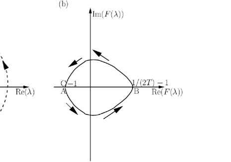
Figure 5: The loop in the complex F𝐹F-plane, (b), corresponding to the loop in the complex λ𝜆\lambda-plane, (a), as determined by the function F(λ)𝐹𝜆F(\lambda) in Eq. (IV.2).

Considering m𝑚m and T𝑇T strictly positive, we multiply for convenience the numerator and denominator of Eq. (IV.2) by mT𝑚𝑇mT to obtain

F(λ;m,T,σ)=emT2Tp=0(mT)p(p+mT)p!𝐹𝜆𝑚𝑇𝜎superscript𝑒𝑚𝑇2𝑇superscriptsubscript𝑝0superscript𝑚𝑇𝑝𝑝𝑚𝑇𝑝\displaystyle F(\lambda;m,T,\sigma)=\frac{e^{mT}}{2T}\sum_{p=0}^{\infty}\frac{\left(-mT\right)^{p}\left(p+mT\right)}{p!}
×g(ω)dωmT+p+mλ+iσmω1=0.\displaystyle\times\frac{g(\omega)\mbox{d}\omega}{mT+p+\sqrt{m}\lambda+i\sigma m\omega}-1=0. (33)

Let us first look for pure imaginary solutions of this equation. Separating into real and imaginary parts, we have

Re[F(iμ;m,T,σ)]=emT2Tp=0(mT)pp!Redelimited-[]𝐹𝑖𝜇𝑚𝑇𝜎superscript𝑒𝑚𝑇2𝑇superscriptsubscript𝑝0superscript𝑚𝑇𝑝𝑝\displaystyle{\rm Re}\left[F(i\mu;m,T,\sigma)\right]=\frac{e^{mT}}{2T}\sum_{p=0}^{\infty}\frac{\left(-mT\right)^{p}}{p!}
×dωg(ω)(p+mT)2(p+mT)2+(mσω+mμ)21=0,\displaystyle\times\int\mbox{d}\omega\,g(\omega)\frac{\left(p+mT\right)^{2}}{\left(p+mT\right)^{2}+\left(m\sigma\omega+\sqrt{m}\mu\right)^{2}}-1=0,
(34)
Im[F(iμ;m,T,σ)]=emT2Tp=0(mT)pp!Imdelimited-[]𝐹𝑖𝜇𝑚𝑇𝜎superscript𝑒𝑚𝑇2𝑇superscriptsubscript𝑝0superscript𝑚𝑇𝑝𝑝\displaystyle{\rm Im}\left[F(i\mu;m,T,\sigma)\right]=-\frac{e^{mT}}{2T}\sum_{p=0}^{\infty}\frac{\left(-mT\right)^{p}}{p!}
×dωg(ω)(p+mT)(mσω+mμ)(p+mT)2+(mσω+mμ)2=0.\displaystyle\times\int\mbox{d}\omega\,g(\omega)\frac{\left(p+mT\right)\left(m\sigma\omega+\sqrt{m}\mu\right)}{\left(p+mT\right)^{2}+\left(m\sigma\omega+\sqrt{m}\mu\right)^{2}}=0. (35)

In the second equation above, we make the change of variables mσω+mμ=mσx𝑚𝜎𝜔𝑚𝜇𝑚𝜎𝑥m\sigma\omega+\sqrt{m}\mu=m\sigma x, and exploit the parity in x𝑥x of the sum, to obtain

Im[F(iμ;m,T,σ)]=Imdelimited-[]𝐹𝑖𝜇𝑚𝑇𝜎absent\displaystyle{\rm Im}\left[F(i\mu;m,T,\sigma)\right]=
mσ0dx{[g(xμmσ)g(xμmσ)]\displaystyle-m\sigma\int_{0}^{\infty}\mbox{d}x\Big{\{}\left[g\left(x-\frac{\mu}{\sqrt{m}\sigma}\right)-g\left(-x-\frac{\mu}{\sqrt{m}\sigma}\right)\right]
×xp=0(mT)pp!p+mT(p+mT)2+m2σ2x2}=0.\displaystyle\times x\sum_{p=0}^{\infty}\frac{\left(-mT\right)^{p}}{p!}\frac{p+mT}{\left(p+mT\right)^{2}+m^{2}\sigma^{2}x^{2}}\Big{\}}=0. (36)

It can be shown that the sum on the right-hand side is positive definite for any finite σ𝜎\sigma. Furthermore, for our class of distribution functions, one may see that the term in square brackets is positive (respectively, negative) definite for μ>0𝜇0\mu>0 (respectively, for μ<0𝜇0\mu<0). As a consequence, the last equation is never satisfied for μ0𝜇0\mu\neq 0 and finite, and therefore, the eigenvalue equation does not admit pure imaginary solutions [the proof holds also for the particular case g(ω)=δ(ω)𝑔𝜔𝛿𝜔g(\omega)=\delta(\omega), as may be checked]. We also conclude that there can be at most one solution with positive real part. In fact, if in the complex λ𝜆\lambda-plane, we perform the loop depicted in Fig. 5(a) (where it is meant that the points A𝐴A and C𝐶C represent Imλ±Im𝜆plus-or-minus{\rm Im}\lambda\to\pm\infty, respectively, and the radius of the arc extends to \infty), then, in the complex-F(λ)𝐹𝜆F(\lambda) plane, we obtain, due to the sign properties of Im[F(iμ;m,T,σ)]Imdelimited-[]𝐹𝑖𝜇𝑚𝑇𝜎{\rm Im}\left[F(i\mu;m,T,\sigma)\right] just described, the loop qualitatively represented in Fig. 5(b). The point F=1𝐹1F=-1 in Fig. 5(b) is obtained for λ𝜆\lambda, in Fig. 5(a), for values at points A𝐴A and C𝐶C and in the whole of the arc extending to infinity. The position of the point B𝐵B in the complex-F𝐹F plane is determined by the value of F(0)𝐹0F(0), which is given by

F(0;m,T,σ)=emT2Tp=0(mT)pp!𝐹0𝑚𝑇𝜎superscript𝑒𝑚𝑇2𝑇superscriptsubscript𝑝0superscript𝑚𝑇𝑝𝑝\displaystyle F(0;m,T,\sigma)=\frac{e^{mT}}{2T}\sum_{p=0}^{\infty}\frac{\left(-mT\right)^{p}}{p!}
dωg(ω)(p+mT)2(p+mT)2+(mσω)21.d𝜔𝑔𝜔superscript𝑝𝑚𝑇2superscript𝑝𝑚𝑇2superscript𝑚𝜎𝜔21\displaystyle\int\mbox{d}\omega\,g(\omega)\frac{\left(p+mT\right)^{2}}{\left(p+mT\right)^{2}+\left(m\sigma\omega\right)^{2}}-1. (37)

From the well-known theorem of complex analysis on the number of roots of a function in a given domain of the complex plane Smirnov:1964 , we therefore obtain that for F(0;m,T,σ)>0𝐹0𝑚𝑇𝜎0F(0;m,T,\sigma)>0, there is one and only one solution of the eigenvalue equation with positive real part; on the other hand, for F(0;m,T,σ)<0𝐹0𝑚𝑇𝜎0F(0;m,T,\sigma)<0, there is no such solution. When the single solution with positive real part exists, it is necessarily real, since a complex solution would imply the existence of its complex conjugate. The value of F(0;m,T,σ)𝐹0𝑚𝑇𝜎F(0;m,T,\sigma) is readily seen to be equal to 1/(2T)112𝑇11/(2T)-1 for σ=0𝜎0\sigma=0. For positive σ𝜎\sigma, the value will depend on the particular form of the distribution function g(ω)𝑔𝜔g(\omega). However, it is possible to prove that the value is always smaller than 1/(2T)112𝑇11/(2T)-1; this is consistent with the physically reasonable fact that if the incoherent state is stable for σ=0𝜎0\sigma=0, which happens for T>1/2𝑇12T>1/2, it is all the more stable for σ>0𝜎0\sigma>0.

The surface delimiting the region of instability in the (m,T,σ)𝑚𝑇𝜎(m,T,\sigma) phase space is implicitly defined by Eq. (IV.2) [i.e. F(0;m,T,σ)=0𝐹0𝑚𝑇𝜎0F(0;m,T,\sigma)=0], which, in principle, can be solved to obtain the threshold value of σ𝜎\sigma (denoted by σincsuperscript𝜎inc\sigma^{\rm inc}) as a function of (m,T)𝑚𝑇(m,T): σinc=σinc(m,T)superscript𝜎incsuperscript𝜎inc𝑚𝑇\sigma^{\rm inc}=\sigma^{\rm inc}(m,T). On physical grounds, we expect that the latter is a single valued function, and that for any given value of m𝑚m, it is a decreasing function of T𝑇T for 0T1/20𝑇120\leq T\leq 1/2, reaching 00 for T=1/2𝑇12T=1/2. We are able to prove analytically these facts for the class of unimodal distribution functions g(ω)𝑔𝜔g(\omega) considered in this work that includes the Gaussian case. However, we can prove in general for any g(ω)𝑔𝜔g(\omega) that σinc(m,T)superscript𝜎inc𝑚𝑇\sigma^{\rm inc}(m,T) tends to 00 for m𝑚m\to\infty. This is done using the integral representation

p=0(mT)pp!(p+mT)2(p+a)2+(mσω)2=emTsuperscriptsubscript𝑝0superscript𝑚𝑇𝑝𝑝superscript𝑝𝑚𝑇2superscript𝑝𝑎2superscript𝑚𝜎𝜔2superscript𝑒𝑚𝑇\displaystyle\sum_{p=0}^{\infty}\frac{\left(-mT\right)^{p}}{p!}\frac{\left(p+mT\right)^{2}}{\left(p+a\right)^{2}+\left(m\sigma\omega\right)^{2}}=e^{-mT} (38)
(mσω)0dtexp[mT(t+et)]sin(mσωt).𝑚𝜎𝜔superscriptsubscript0d𝑡𝑚𝑇𝑡superscript𝑒𝑡𝑚𝜎𝜔𝑡\displaystyle-\left(m\sigma\omega\right)\int_{0}^{\infty}\mbox{d}t\,\exp\left[-mT\left(t+e^{-t}\right)\right]\sin\left(m\sigma\omega t\right).

For σ>0𝜎0\sigma>0 and m𝑚m\to\infty, one may see that the term within the integral in the last equation tends to emTsuperscript𝑒𝑚𝑇e^{-mT}. We thus obtain by examining Eq. (IV.2) that F(0;m,T>0,σ>0)=1F(0;m\to\infty,T>0,\sigma>0)=-1. Combined with the fact that F(0;m,T,0)=1/(2T)1𝐹0𝑚𝑇012𝑇1F(0;m,T,0)=1/(2T)-1, this shows that σinc(m,0T1/2)=0superscript𝜎incformulae-sequence𝑚0𝑇120\sigma^{\rm inc}(m\to\infty,0\leq T\leq 1/2)=0.

Let us now turn to the Gaussian case, g(ω)=12πexp[ω22]𝑔𝜔12𝜋superscript𝜔22g(\omega)=\frac{1}{\sqrt{2\pi}}\exp\left[-\frac{\omega^{2}}{2}\right]. Denoting with a subscript g𝑔g in this case, and using Eq. (38), we have

Fg(0;m,T,σ)=12T1emT2T2πdωeω22(mσω)subscript𝐹𝑔0𝑚𝑇𝜎12𝑇1superscript𝑒𝑚𝑇2𝑇2𝜋d𝜔superscript𝑒superscript𝜔22𝑚𝜎𝜔\displaystyle F_{g}(0;m,T,\sigma)=\frac{1}{2T}-1-\frac{e^{mT}}{2T\sqrt{2\pi}}\int\mbox{d}\omega\,e^{-\frac{\omega^{2}}{2}}\left(m\sigma\omega\right)
×0dtexp[mT(t+et)]sin(mσωt).\displaystyle\times\int_{0}^{\infty}\mbox{d}t\,\exp\left[-mT\left(t+e^{-t}\right)\right]\sin\left(m\sigma\omega t\right). (39)

The integral in ω𝜔\omega can be easily performed. Making the change of variable mσt=y𝑚𝜎𝑡𝑦m\sigma t=y, we arrive at the following equation:

Fg(0;m,T,σ)=12T1subscript𝐹𝑔0𝑚𝑇𝜎12𝑇1\displaystyle F_{g}(0;m,T,\sigma)=\frac{1}{2T}-1
12T0dyyey22exp[mT(1ymσeymσ)].12𝑇superscriptsubscript0d𝑦𝑦superscript𝑒superscript𝑦22𝑚𝑇1𝑦𝑚𝜎superscript𝑒𝑦𝑚𝜎\displaystyle-\frac{1}{2T}\int_{0}^{\infty}\mbox{d}y\,ye^{-\frac{y^{2}}{2}}\exp\left[mT\left(1-\frac{y}{m\sigma}-e^{-\frac{y}{m\sigma}}\right)\right]. (40)

The equation Fg(0;m,T,σ)=0subscript𝐹𝑔0𝑚𝑇𝜎0F_{g}(0;m,T,\sigma)=0 defines implicitly the function σinc(m,T)superscript𝜎inc𝑚𝑇\sigma^{\rm inc}(m,T). We can show that this is a single-valued function with the properties σincm<0superscript𝜎inc𝑚0\frac{\partial\sigma^{\rm inc}}{\partial m}<0 and σincT<0superscript𝜎inc𝑇0\frac{\partial\sigma^{\rm inc}}{\partial T}<0. We show this by explicitly computing the partial derivatives of Fg(0;m,T,σ)subscript𝐹𝑔0𝑚𝑇𝜎F_{g}(0;m,T,\sigma) with respect to m𝑚m and σ𝜎\sigma, and by evaluating the behavior with respect to changes in T𝑇T by adopting a suitable strategy. We begin by computing the derivative with respect to σ𝜎\sigma. From Eq. (IV.2), we readily obtain

σFg(0;m,T,σ)=12σ20dyy2ey22(1eymσ)𝜎subscript𝐹𝑔0𝑚𝑇𝜎12superscript𝜎2superscriptsubscript0d𝑦superscript𝑦2superscript𝑒superscript𝑦221superscript𝑒𝑦𝑚𝜎\displaystyle\frac{\partial}{\partial\sigma}F_{g}(0;m,T,\sigma)=-\frac{1}{2\sigma^{2}}\int_{0}^{\infty}\mbox{d}y\,y^{2}e^{-\frac{y^{2}}{2}}\left(1-e^{-\frac{y}{m\sigma}}\right)
×exp[mT(1ymσeymσ)],absent𝑚𝑇1𝑦𝑚𝜎superscript𝑒𝑦𝑚𝜎\displaystyle\times\exp\left[mT\left(1-\frac{y}{m\sigma}-e^{-\frac{y}{m\sigma}}\right)\right], (41)

which is clearly negative. Second, the derivative with respect to m𝑚m gives

mFg(0;m,T,σ)=120dyyey22𝑚subscript𝐹𝑔0𝑚𝑇𝜎12superscriptsubscript0d𝑦𝑦superscript𝑒superscript𝑦22\displaystyle\frac{\partial}{\partial m}F_{g}(0;m,T,\sigma)=-\frac{1}{2}\int_{0}^{\infty}\mbox{d}y\,ye^{-\frac{y^{2}}{2}}
×(1eymσymσeymσ)exp[mT(1ymσeymσ)].absent1superscript𝑒𝑦𝑚𝜎𝑦𝑚𝜎superscript𝑒𝑦𝑚𝜎𝑚𝑇1𝑦𝑚𝜎superscript𝑒𝑦𝑚𝜎\displaystyle\times\left(1-e^{-\frac{y}{m\sigma}}-\frac{y}{m\sigma}e^{-\frac{y}{m\sigma}}\right)\exp\left[mT\left(1-\frac{y}{m\sigma}-e^{-\frac{y}{m\sigma}}\right)\right].

This derivative is negative, since 1exxex1superscript𝑒𝑥𝑥superscript𝑒𝑥1-e^{-x}-xe^{-x} is positive for x>0𝑥0x>0. From the implicit function theorems, we then derive that σincm<0superscript𝜎inc𝑚0\frac{\partial\sigma^{\rm inc}}{\partial m}<0. The study of the behavior with respect to a change in T𝑇T is a bit more complicated. Since we are considering T>0𝑇0T>0, we multiply Eq. (IV.2) by 2T2𝑇2T to obtain

2TFg(0;m,T,σ)=12T2𝑇subscript𝐹𝑔0𝑚𝑇𝜎12𝑇\displaystyle 2TF_{g}(0;m,T,\sigma)=1-2T
0dyyey22exp[mT(1ymσeymσ)].superscriptsubscript0d𝑦𝑦superscript𝑒superscript𝑦22𝑚𝑇1𝑦𝑚𝜎superscript𝑒𝑦𝑚𝜎\displaystyle-\int_{0}^{\infty}\mbox{d}y\,ye^{-\frac{y^{2}}{2}}\exp\left[mT\left(1-\frac{y}{m\sigma}-e^{-\frac{y}{m\sigma}}\right)\right]. (43)

Let us consider the integral on the right-hand side

0dyyey22exp[mT(1ymσeymσ)].superscriptsubscript0d𝑦𝑦superscript𝑒superscript𝑦22𝑚𝑇1𝑦𝑚𝜎superscript𝑒𝑦𝑚𝜎\int_{0}^{\infty}\mbox{d}y\,ye^{-\frac{y^{2}}{2}}\exp\left[mT\left(1-\frac{y}{m\sigma}-e^{-\frac{y}{m\sigma}}\right)\right]. (44)

Since 1xex1𝑥superscript𝑒𝑥1-x-e^{-x} is negative for x>0𝑥0x>0, we conclude that the T𝑇T derivative of this expression is negative, while its second T𝑇T derivative is positive. Then the right-hand side of Eq. (IV.2) can be zero, for T>0𝑇0T>0, for at most one value of T𝑇T. Furthermore, since for fixed y𝑦y and m𝑚m the value of y/(mσ)𝑦𝑚𝜎y/(m\sigma) decreases if σ𝜎\sigma increases, the T𝑇T value for which Fg(0;m,T,σ)=0subscript𝐹𝑔0𝑚𝑇𝜎0F_{g}(0;m,T,\sigma)=0 decreases for increasing σ𝜎\sigma at fixed m𝑚m. This concludes the proof. Furthermore, for what we have seen before, σinc(m,1/2)=0superscript𝜎inc𝑚120\sigma^{\rm inc}(m,1/2)=0 and limmσinc(m,T)=0subscript𝑚superscript𝜎inc𝑚𝑇0\lim_{m\to\infty}\sigma^{\rm inc}(m,T)=0 for 0T1/20𝑇120\leq T\leq 1/2.

From the above analysis, it should be clear that the proof is not restricted to the Gaussian case, but would work exactly in the same way for any g(ω)𝑔𝜔g(\omega) such that

βdxg(x)xsin(βx),𝛽d𝑥𝑔𝑥𝑥𝛽𝑥\beta\int\mbox{d}x\,g(x)x\sin(\beta x), (45)

is positive for any β𝛽\beta. However, on physical grounds, we are led to assume that the same conclusions hold for any unimodal g(ω)𝑔𝜔g(\omega).

On the basis of our analysis, it follows that at the point of neutral stability, one has λ=0𝜆0\lambda=0, which when substituted in Eq. (31) gives σinc(m,T)superscript𝜎inc𝑚𝑇\sigma^{\rm inc}(m,T) to be satisfying

2TemT=p=0(mT)p(1+pmT)2p!g(ω)dω(1+pmT)2+(σinc)2ω2T2.2𝑇superscript𝑒𝑚𝑇superscriptsubscript𝑝0superscript𝑚𝑇𝑝superscript1𝑝𝑚𝑇2𝑝superscriptsubscript𝑔𝜔d𝜔superscript1𝑝𝑚𝑇2superscriptsuperscript𝜎inc2superscript𝜔2superscript𝑇2\frac{2T}{e^{mT}}=\sum_{p=0}^{\infty}\frac{(-mT)^{p}(1+\frac{p}{mT})^{2}}{p!}\int\limits_{-\infty}^{\infty}\frac{g(\omega)\mbox{d}\omega}{(1+\frac{p}{mT})^{2}+\frac{(\sigma^{\rm inc})^{2}\omega^{2}}{T^{2}}}. (46)

In the (m,T,σ)𝑚𝑇𝜎(m,T,\sigma) space, Eq. (46) defines the stability surface σinc(m,T)superscript𝜎inc𝑚𝑇\sigma^{\rm inc}(m,T). There will similarly be the stability surface σcoh(m,T)superscript𝜎coh𝑚𝑇\sigma^{\rm coh}(m,T) (see Fig. 1(d) which shows the two surfaces as obtained in N𝑁N-body simulations for N=500𝑁500N=500 for a Gaussian g(ω)𝑔𝜔g(\omega)). The two surfaces coincide on the critical lines on the (T,σ)𝑇𝜎(T,\sigma) and (m,T)𝑚𝑇(m,T) planes where the transition becomes continuous; outside these planes, the surfaces enclose the first-order transition surface σc(m,T)subscript𝜎𝑐𝑚𝑇\sigma_{c}(m,T) i.e., σcoh(m,T)>σc(m,T)>σinc(m,T)superscript𝜎coh𝑚𝑇subscript𝜎𝑐𝑚𝑇superscript𝜎inc𝑚𝑇\sigma^{\rm coh}(m,T)>\sigma_{c}(m,T)>\sigma^{\rm inc}(m,T). We now show by taking limits that the surface σinc(m,T)superscript𝜎inc𝑚𝑇\sigma^{\rm inc}(m,T) meets the critical lines on the (T,σ)𝑇𝜎(T,\sigma) and (m,T)𝑚𝑇(m,T) planes, and also obtain its intersection with the (m,σ)𝑚𝜎(m,\sigma)-plane. On considering m0𝑚0m\to 0 at a fixed T𝑇T, only the p=0𝑝0p=0 term in the sum in Eq. (46) contributes, giving

limm0,Tfixedσinc(m,T)=σc(m=0,T),subscript𝑚0𝑇fixedsuperscript𝜎inc𝑚𝑇subscript𝜎𝑐𝑚0𝑇\lim_{m\to 0,T\,{\rm fixed}}\sigma^{\rm inc}(m,T)=\sigma_{c}(m=0,T), (47)

with the implicit expression of σc(m=0,T)subscript𝜎𝑐𝑚0𝑇\sigma_{c}(m=0,T) given by Eq. (17). Similarly, one finds that

limTTc,mfixedσinc(m,T)=0,subscript𝑇superscriptsubscript𝑇𝑐𝑚fixedsuperscript𝜎inc𝑚𝑇0\lim_{T\to T_{c}^{-},m\,{\rm fixed}}\sigma^{\rm inc}(m,T)=0, (48)

that is, on the (m,T)𝑚𝑇(m,T) plane, the transition line is given by Tc=1/2subscript𝑇𝑐12T_{c}=1/2. When T0𝑇0T\to 0 at a fixed m𝑚m, we get

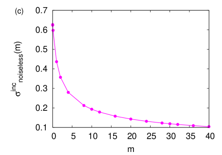
σnoiselessinc(m)limT0,mfixedσinc(m,T),subscriptsuperscript𝜎incnoiseless𝑚subscript𝑇0𝑚fixedsuperscript𝜎inc𝑚𝑇\sigma^{\rm inc}_{\rm noiseless}(m)\equiv\lim_{T\to 0,m\,{\rm fixed}}\sigma^{\rm inc}(m,T), (49)

with

1=πg(0)2σnoiselessincm2g(ω)dω1+m2(σnoiselessinc)2ω2.1𝜋𝑔02subscriptsuperscript𝜎incnoiseless𝑚2superscriptsubscript𝑔𝜔d𝜔1superscript𝑚2superscriptsubscriptsuperscript𝜎incnoiseless2superscript𝜔2\displaystyle 1=\frac{\pi g(0)}{2\sigma^{\rm inc}_{\rm noiseless}}-\frac{m}{2}\int_{-\infty}^{\infty}\frac{g(\omega)\mbox{d}\omega}{1+m^{2}(\sigma^{\rm inc}_{\rm noiseless})^{2}\omega^{2}}. (50)
Refer to caption
Figure 6: (Color online) The figure shows the limit Eq. (49) for the case of a Gaussian g(ω)𝑔𝜔g(\omega) with zero mean and unit width.

For the case of a Gaussian g(ω)𝑔𝜔g(\omega), the limits (47) and (48) are shown in Figs. 1(b) and 1(c), while the limit Eq. (49) is shown in Fig. 6.

V Comparison with numerics

For a Gaussian g(ω)𝑔𝜔g(\omega), Eq. (46) gives

1=emTπ22σincp=0(mT)p(1+pmT)p!eT2(1+p/mT)22(σinc)2Erfc[T(1+pmT)σinc2].1superscript𝑒𝑚𝑇𝜋22superscript𝜎incsuperscriptsubscript𝑝0superscript𝑚𝑇𝑝1𝑝𝑚𝑇𝑝superscript𝑒superscript𝑇2superscript1𝑝𝑚𝑇22superscriptsuperscript𝜎inc2Erfcdelimited-[]𝑇1𝑝𝑚𝑇superscript𝜎inc21=\frac{e^{mT}\sqrt{\pi}}{2\sqrt{2}\sigma^{\rm inc}}\sum_{p=0}^{\infty}\frac{(-mT)^{p}(1+\frac{p}{mT})}{p!e^{-\frac{T^{2}(1+p/mT)^{2}}{2(\sigma^{\rm inc})^{2}}}}{\rm Erfc}\Big{[}\frac{T(1+\frac{p}{mT})}{\sigma^{\rm inc}\sqrt{2}}\Big{]}. (51)

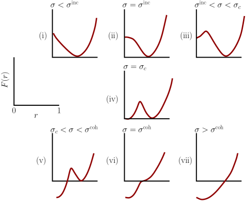
Choosing m=20𝑚20m=20 and T=0.25𝑇0.25T=0.25, the above equation gives σinc(m,T)0.10076superscript𝜎inc𝑚𝑇0.10076\sigma^{\rm inc}(m,T)\approx 0.10076. Then, preparing the system in the incoherent stationary state at a given σ𝜎\sigma, our theoretical analysis predicts that r𝑟r, in the dynamically unstable regime of the incoherent state (i.e., with σ<σinc𝜎superscript𝜎inc\sigma<\sigma^{\rm inc}), relaxes at long times to its steady-state value corresponding to the synchronized phase. For σ>σinc(m,T)𝜎superscript𝜎inc𝑚𝑇\sigma>\sigma^{\rm inc}(m,T), when the incoherent initial state is linearly stable, r𝑟r is zero for all times. We now compare the above continuum-limit predictions with N𝑁N-body simulations. We monitor the evolution of r𝑟r in time while starting from the incoherent stationary state. To discuss the results, we employ the standard picture of phase transitions occurring dynamically as the dissipative relaxation of the order parameter towards the minimum of a phenomenological Landau free energy Binder:1987 . For a first-order phase transition, we draw in Fig. 7 the corresponding schematic free energy F(r)𝐹𝑟F(r) versus r𝑟r for fixed m𝑚m and T𝑇T at different σ𝜎\sigma’s footnote . The picture helps to explain, e.g., the flips in r𝑟r in Fig. 4, which correspond to dynamics at σ𝜎\sigma close to σcsubscript𝜎𝑐\sigma_{c}, when the system switches back and forth between the two almost stable synchronized and incoherent states.
Refer to caption
Figure 7: (Color online) Schematic Landau free energy F(r)𝐹𝑟F(r) versus r𝑟r for first-order transitions at fixed m𝑚m and T𝑇T while varying σ𝜎\sigma. Panels (i) and (vii) correspond to the synchronized and incoherent phase being at the global minimum. In panel (iii) (respectively, (v)), the synchronized (respectively, incoherent) phase is at the global minimum, while the incoherent (respectively, synchronized) phase is at a local minimum, hence, metastable. Panel (iv) corresponds to the first-order transition point, with the two phases coexisting at two minima of equal heights.
Refer to caption
Refer to caption
Refer to caption
Refer to caption
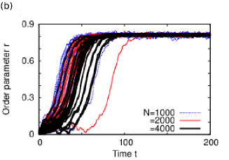
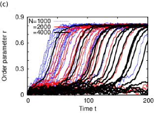
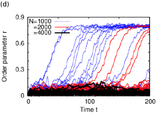
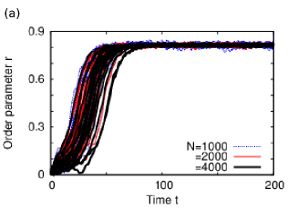
Figure 8: (Color online) Panels (a)-(d) show r𝑟r vs. time at m=20,T=0.25formulae-sequence𝑚20𝑇0.25m=20,T=0.25 for four values of σ𝜎\sigma, two below ((a): σ=0.09𝜎0.09\sigma=0.09, (b): σ=0.095𝜎0.095\sigma=0.095), and two above ((c): σ=0.11𝜎0.11\sigma=0.11, (d): σ=0.12𝜎0.12\sigma=0.12) the theoretical threshold σinc(m,T)0.10076superscript𝜎inc𝑚𝑇0.10076\sigma^{\rm inc}(m,T)\approx 0.10076. The data are obtained in N𝑁N-body simulations for a Gaussian g(ω)𝑔𝜔g(\omega) with zero mean and unit width.

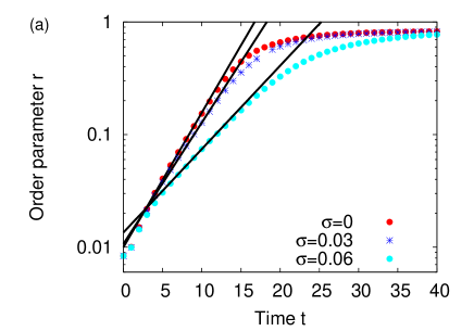
Let us investigate the dynamics for σ𝜎\sigma around σinc(m,T)superscript𝜎inc𝑚𝑇\sigma^{\rm inc}(m,T). Figures 8(a)-(d) show simulation results for r𝑟r versus time for four values of σ𝜎\sigma, two below and two above σinc(m,T)superscript𝜎inc𝑚𝑇\sigma^{\rm inc}(m,T). In each case, we display the dependence for 202020 realizations of the initial incoherent state for three values of N𝑁N. Figure 8(a) for σ<σinc(m,T)𝜎superscript𝜎inc𝑚𝑇\sigma<\sigma^{\rm inc}(m,T) illustrates that the system while starting from the unstable incoherent state settles down in time into the globally stable synchronized state; this corresponds to dynamics in the landscape in Fig. 7(i). The relaxation of r𝑟r from the initial to final synchronized state value occurs exponentially fast in time as eλtsuperscript𝑒𝜆𝑡e^{\lambda t}; the growth rate λ𝜆\lambda is obtained from Eq. (31) after substituting a Gaussian distribution for g(ω)𝑔𝜔g(\omega). In Fig. 9, we demonstrate a match of λ𝜆\lambda in theory and simulations.

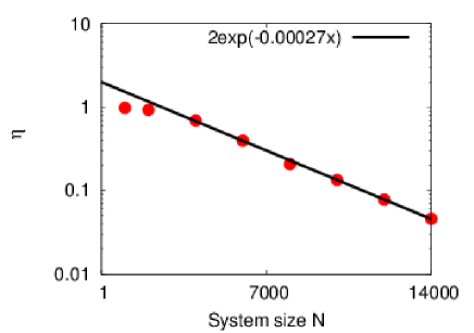
In Fig. 8(b), when σ𝜎\sigma is larger than in Fig. 8(a), yet below σinc(m,T)superscript𝜎inc𝑚𝑇\sigma^{\rm inc}(m,T), the system settles at long times into the synchronized state for all realizations. Yet, some of them, at short times, tend to stay in the initial incoherent state due to finite-N𝑁N effects not captured by our continuum limit theory; see Eq. (27). For σ>σinc(m,T)𝜎superscript𝜎inc𝑚𝑇\sigma>\sigma^{\rm inc}(m,T), but σ<σc(m,T)𝜎subscript𝜎𝑐𝑚𝑇\sigma<\sigma_{c}(m,T), we expect on the basis of the landscape sketched in Fig. 7(iii) that the system settles at long times into the globally stable synchronized state, while for finite times, remains trapped in the metastable incoherent state. Indeed, Fig. 8(c) shows that most realizations relax to synchronized states. However, as N𝑁N increases, the number of realizations staying close to the initial incoherent state for a finite time increases. We found that the fraction η𝜂\eta of realizations relaxing to synchronized state within a fixed time decreases exponentially fast in N𝑁N for large N𝑁N; see Fig. 10. This observation implies that for the fixed time of observation, there exists a larger N𝑁N than the ones in Fig. 8(c) for which all realizations remain close to the incoherent state; it then follows that in the continuum limit, all realizations stay close to the incoherent state.

To explain the above mentioned behavior of η𝜂\eta with N𝑁N, let us first consider the noisy dynamics of a single particle on a potential landscape, when the typical time to get out of a metastable state is given in the weak-noise limit by the Kramers time, i.e., an exponential in the ratio of the potential energy barrier to come out of the metastable state to the strength of the noise Kramers:1940 . For the dynamics of the order parameter on a free-energy landscape for mean-field systems, the escape time out of a metastable state obeys Kramers formula with the value of the free-energy barrier replacing the potential energy barrier, and with an extra factor of N𝑁N multiplying the barrier height Griffiths:1966 ; this explains Fig. 8(c) and the behavior of η𝜂\eta.

Figure 8(d), for σ𝜎\sigma larger than σinc(m,T)superscript𝜎inc𝑚𝑇\sigma^{\rm inc}(m,T) than in Fig. 8(c), shows that with respect to (c), more realizations stay close to the initial incoherent state for longer times, due to a larger barrier between the incoherent and synchronized state. On the basis of the above discussions, we conclude that our theoretical predictions are borne out by our simulation results. In particular, the simulation results for N=500𝑁500N=500 suggest that the stability threshold of the incoherent state lies in between σ=0.095𝜎0.095\sigma=0.095 and σ=0.11𝜎0.11\sigma=0.11, a range that includes its theoretical continuum-limit value (0.10076absent0.10076\approx 0.10076).

Refer to caption
Refer to caption
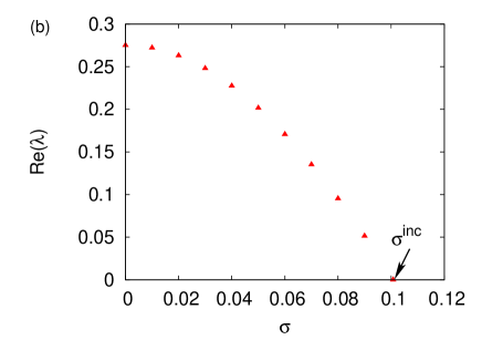
Figure 9: (Color online) (a) Simulation results denoted by points, demonstrating exponentially fast relaxation eλtsimilar-toabsentsuperscript𝑒𝜆𝑡\sim e^{\lambda t} of r𝑟r from its initial incoherent state value to its final synchronized state value for values of σ𝜎\sigma below σinc(m,T)0.10076superscript𝜎inc𝑚𝑇0.10076\sigma^{\rm inc}(m,T)\approx 0.10076 for a Gaussian g(ω)𝑔𝜔g(\omega) with m=20,T=0.25,N=104formulae-sequence𝑚20formulae-sequence𝑇0.25𝑁superscript104m=20,T=0.25,N=10^{4}; the black solid lines denote exponential growth with theoretically computed growth rates λ𝜆\lambda obtained from Eq. (31) for a Gaussian g(ω)𝑔𝜔g(\omega) with zero mean and unit width. The simulation data are obtained from N𝑁N-body simulation for a Gaussian g(ω)𝑔𝜔g(\omega) with zero mean and unit width. (b) Theoretical λ𝜆\lambda as a function of σ𝜎\sigma for the same m𝑚m and T𝑇T values; in particular, λ𝜆\lambda hits zero at the stability threshold σinc(m,T)superscript𝜎inc𝑚𝑇\sigma^{\rm inc}(m,T).
Refer to caption
Figure 10: (Color online) For m=20,T=0.25,σ=0.11formulae-sequence𝑚20formulae-sequence𝑇0.25𝜎0.11m=20,T=0.25,\sigma=0.11, the figure shows the fraction η𝜂\eta of realizations of initial incoherent state relaxing to synchronized state within the fixed time of observation t=200𝑡200t=200, for a value of σ𝜎\sigma above σinc(m,T)superscript𝜎inc𝑚𝑇\sigma^{\rm inc}(m,T), for which the incoherent phase is linearly stable in the continuum limit. The figure shows that η𝜂\eta for large N𝑁N decreases exponentially fast with increase of N𝑁N. The data are obtained in N𝑁N-body simulations for a Gaussian g(ω)𝑔𝜔g(\omega) with zero mean and unit width.

VI Conclusions

To summarize, we considered an extension of the Kuramoto model that includes an inertial term and a stochastic noise. For a general unimodal frequency distribution, we obtained the complete phase diagram of the model, demarcating parameter ranges to observe synchronization. We showed that the system displays a nonequilibrium first-order transition from a synchronized phase at low parameter values to an incoherent phase at high values. The phase diagram contains all previous results derived in specific limits of the dynamics. While we provided strong numerical evidence for the existence of both the synchronized and the incoherent phase, only the latter could be treated analytically to obtain the corresponding linear stability threshold that bounds the first-order transition point from below. It would be interesting to consider possible extension of our studies to systems with non-mean-field couplings, taking hints from similar previous studies in specific limits of the dynamics Campa:2003 ; Bachelard:2011 ; Gupta:2012 ; Gupta:2012-1 .

We acknowledge fruitful discussions with T. Dauxois, D. Mukamel, C. Nardini, A. Patelli and H. Touchette, support of ENS-Lyon and the grants CEFIPRA 4604-3 and ANR-10-CEXC-010-01.

Appendix A Proof that the dynamics Eq. (12) does not satisfy detailed balance

In this section, we prove that the dynamics Eq. (12) does not satisfy detailed balance unless g(ω)=δ(ω)𝑔𝜔𝛿𝜔g(\omega)=\delta(\omega), thus σ𝜎\sigma is zero. For simplicity, we discuss the proof here for the case of two distinct natural frequencies [bimodal g(ω)𝑔𝜔g(\omega)]. Let us say that in a given realization of g(ω)𝑔𝜔g(\omega), there are N1subscript𝑁1N_{1} oscillators with natural frequencies ω1subscript𝜔1\omega_{1}, and N2subscript𝑁2N_{2} oscillators with natural frequencies ω2subscript𝜔2\omega_{2}, where N1+N2=Nsubscript𝑁1subscript𝑁2𝑁N_{1}+N_{2}=N.

To prove that the dynamics Eq. (12) does not satisfy detailed balance unless σ=0𝜎0\sigma=0, we rewrite the Fokker-Planck Eq. (20) as

fN(𝐱)t=i=12N(Ai(𝐱)fN(𝐱))xisubscript𝑓𝑁𝐱𝑡superscriptsubscript𝑖12𝑁subscript𝐴𝑖𝐱subscript𝑓𝑁𝐱subscript𝑥𝑖\displaystyle\frac{\partial f_{N}(\mathbf{x})}{\partial t}=-\sum_{i=1}^{2N}\frac{\partial(A_{i}(\mathbf{x})f_{N}(\mathbf{x}))}{\partial x_{i}}
+12i,j=12N2(Bi,j(𝐱)fN(𝐱))xixj,12superscriptsubscript𝑖𝑗12𝑁superscript2subscript𝐵𝑖𝑗𝐱subscript𝑓𝑁𝐱subscript𝑥𝑖subscript𝑥𝑗\displaystyle+\frac{1}{2}\sum_{i,j=1}^{2N}\frac{\partial^{2}(B_{i,j}(\mathbf{x})f_{N}(\mathbf{x}))}{\partial x_{i}\partial x_{j}}, (52)

where

xi={θi;i=1,2,,N,viN;i=N+1,,2N,subscript𝑥𝑖casesformulae-sequencesubscript𝜃𝑖𝑖12𝑁missing-subexpressionformulae-sequencesubscript𝑣𝑖𝑁𝑖𝑁12𝑁missing-subexpressionx_{i}=\left\{\begin{array}[]{ll}\theta_{i};i=1,2,\dots,N,\\ v_{i-N};i=N+1,\dots,2N,\end{array}\right.\\ (53)

and

𝐱𝐱\displaystyle\mathbf{x} ={xi}1i2N.absentsubscriptsubscript𝑥𝑖1𝑖2𝑁\displaystyle=\{x_{i}\}_{1\leq i\leq 2N}. (54)

In Eq. (52), the drift vector Ai(𝐱)subscript𝐴𝑖𝐱A_{i}(\mathbf{x}) is given by

Ai(𝐱)={vi;i=1,2,,N,1mviN+1Nj=1Nsin(θjθiN)+σ(ΩT)iN;i=N+1,,2N,subscript𝐴𝑖𝐱casesformulae-sequencesubscript𝑣𝑖𝑖12𝑁missing-subexpression1𝑚subscript𝑣𝑖𝑁1𝑁superscriptsubscript𝑗1𝑁subscript𝜃𝑗subscript𝜃𝑖𝑁missing-subexpressionformulae-sequence𝜎subscriptsuperscriptΩ𝑇𝑖𝑁𝑖𝑁12𝑁missing-subexpressionA_{i}(\mathbf{x})=\left\{\begin{array}[]{ll}v_{i};i=1,2,\dots,N,\\ -\frac{1}{\sqrt{m}}v_{i-N}+\frac{1}{N}\sum_{j=1}^{N}\sin(\theta_{j}-\theta_{i-N})\\ +\sigma\Big{(}\Omega^{T}\Big{)}_{i-N};i=N+1,\dots,2N,\end{array}\right.\\ (55)

while the diffusion matrix is

Bi,j(𝐱)={2Tmδij;i,j>N,0,Otherwise.subscript𝐵𝑖𝑗𝐱cases2𝑇𝑚subscript𝛿𝑖𝑗𝑖𝑗𝑁missing-subexpression0Otherwisemissing-subexpressionB_{i,j}(\mathbf{x})=\left\{\begin{array}[]{ll}\frac{2T}{\sqrt{m}}\delta_{ij};i,j>N,\\ 0,~{}{\rm Otherwise.}\end{array}\right.\\ (56)

The dynamics described by the Fokker-Planck equation of the form Eq. (52) satisfies detailed balance if and only if the following conditions are satisfied Gardiner:1983 :

ϵiϵjBi,j(ϵ𝐱)=Bi,j(𝐱),subscriptitalic-ϵ𝑖subscriptitalic-ϵ𝑗subscript𝐵𝑖𝑗italic-ϵ𝐱subscript𝐵𝑖𝑗𝐱\displaystyle\epsilon_{i}\epsilon_{j}B_{i,j}(\epsilon\mathbf{x})=B_{i,j}(\mathbf{x}), (57)
ϵiAi(ϵ𝐱)fNs(𝐱)=Ai(𝐱)fNs(𝐱)+j=12NBi,j(𝐱)fNs(𝐱)xj,subscriptitalic-ϵ𝑖subscript𝐴𝑖italic-ϵ𝐱superscriptsubscript𝑓𝑁𝑠𝐱subscript𝐴𝑖𝐱superscriptsubscript𝑓𝑁𝑠𝐱superscriptsubscript𝑗12𝑁subscript𝐵𝑖𝑗𝐱superscriptsubscript𝑓𝑁𝑠𝐱subscript𝑥𝑗\displaystyle\epsilon_{i}A_{i}(\epsilon\mathbf{x})f_{N}^{s}(\mathbf{x})=-A_{i}(\mathbf{x})f_{N}^{s}(\mathbf{x})+\sum_{j=1}^{2N}\frac{\partial B_{i,j}(\mathbf{x})f_{N}^{s}(\mathbf{x})}{\partial x_{j}},
(58)

where fNs(𝐱)superscriptsubscript𝑓𝑁𝑠𝐱f_{N}^{s}(\mathbf{x}) is the stationary solution of Eq. (52). Here, ϵi=±1subscriptitalic-ϵ𝑖plus-or-minus1\epsilon_{i}=\pm 1 is a constant that denotes the parity with respect to time reversal of the variables xisubscript𝑥𝑖x_{i}s: Under time reversal, the latter transform as xiϵixisubscript𝑥𝑖subscriptitalic-ϵ𝑖subscript𝑥𝑖x_{i}\rightarrow\epsilon_{i}x_{i}, where ϵi=1subscriptitalic-ϵ𝑖1\epsilon_{i}=-1 or +11+1 depending on whether xisubscript𝑥𝑖x_{i} is odd or even under time reversal. In our case, θisubscript𝜃𝑖\theta_{i}s are even, while visubscript𝑣𝑖v_{i}s are odd.

Using Eq. (56), we see that the condition Eq. (57) is trivially satisfied for our model. To check the other condition, we formally solve Eq. (58) for fNs(𝐱)superscriptsubscript𝑓𝑁𝑠𝐱f_{N}^{s}(\mathbf{x}) and check if the solution solves Eq. (52) in the stationary state. From Eq. (58), we see that for i=1,2,,N𝑖12𝑁i=1,2,\dots,N, the condition reduces to

ϵiAi(ϵ𝐱)fNs(𝐱)subscriptitalic-ϵ𝑖subscript𝐴𝑖italic-ϵ𝐱superscriptsubscript𝑓𝑁𝑠𝐱\displaystyle\epsilon_{i}A_{i}(\epsilon\mathbf{x})f_{N}^{s}(\mathbf{x}) =Ai(𝐱)fNs(𝐱),absentsubscript𝐴𝑖𝐱superscriptsubscript𝑓𝑁𝑠𝐱\displaystyle=-A_{i}(\mathbf{x})f_{N}^{s}(\mathbf{x}), (59)

which, using Eq. (55), is obviously satisfied. For i=N+1,,2N𝑖𝑁12𝑁i=N+1,\dots,2N, we have

vkfNs(𝐱)subscript𝑣𝑘superscriptsubscript𝑓𝑁𝑠𝐱\displaystyle v_{k}f_{N}^{s}(\mathbf{x}) =TfNs(𝐱)vk;k=iN.formulae-sequenceabsent𝑇superscriptsubscript𝑓𝑁𝑠𝐱subscript𝑣𝑘𝑘𝑖𝑁\displaystyle=-\frac{T\partial f_{N}^{s}(\mathbf{x})}{\partial v_{k}};k=i-N. (60)

Solving Eq. (60), we get

fNs(𝐱)superscriptsubscript𝑓𝑁𝑠𝐱\displaystyle f_{N}^{s}(\mathbf{x}) d(θ1,θ2,,θN)exp[12Tk=1Nvk2],proportional-toabsent𝑑subscript𝜃1subscript𝜃2subscript𝜃𝑁12𝑇superscriptsubscript𝑘1𝑁superscriptsubscript𝑣𝑘2\displaystyle\propto d(\theta_{1},\theta_{2},\dots,\theta_{N})\exp\Big{[}-\frac{1}{2T}\sum_{k=1}^{N}v_{k}^{2}\Big{]},

where d(θ1,θ2,,θN)𝑑subscript𝜃1subscript𝜃2subscript𝜃𝑁d(\theta_{1},\theta_{2},\dots,\theta_{N}) is a yet undetermined function. Substituting Eq. (LABEL:eq:stationary-soln1) into Eq. (52), and requiring that it is a stationary solution, we get that σ𝜎\sigma has to be equal to zero and that d(θ1,θ2,,θN)=exp(12NTi,j=1N[1cos(θiθj)])𝑑subscript𝜃1subscript𝜃2subscript𝜃𝑁12𝑁𝑇superscriptsubscript𝑖𝑗1𝑁delimited-[]1subscript𝜃𝑖subscript𝜃𝑗d(\theta_{1},\theta_{2},\dots,\theta_{N})=\exp\Big{(}-\frac{1}{2NT}\sum_{i,j=1}^{N}\Big{[}1-\cos(\theta_{i}-\theta_{j})\Big{]}\Big{)}. Thus, for σ=0𝜎0\sigma=0, when the dynamics reduces to that of the BMF model, we get the stationary solution as

fN,σ=0s(𝐳)exp[HT].proportional-tosuperscriptsubscript𝑓𝑁𝜎0𝑠𝐳𝐻𝑇f_{N,\sigma=0}^{s}(\mathbf{z})\propto\exp\Big{[}-\frac{H}{T}\Big{]}. (62)

where H𝐻H is the Hamiltonian (expressed in terms of dimensionless variables introduced above). The lack of detailed balance for σ0𝜎0\sigma\neq 0 obviously extends to any distribution g(ω)𝑔𝜔g(\omega).

Appendix B Simulation details

Here we describe the method to simulate the dynamics Eq. (12) for given values of m,T,σ𝑚𝑇𝜎m,T,\sigma (note that we are dropping overbars for simplicity of notation), and for a given realization of ωisubscript𝜔𝑖\omega_{i}’s, by employing a numerical integration scheme Gupta:2012-2 . To simulate the dynamics over a time interval [0:𝒯]delimited-[]:0𝒯[0:\mathcal{T}], we first choose a time step size Δt1much-less-thanΔ𝑡1\Delta t\ll 1. Next, we set tn=nΔtsubscript𝑡𝑛𝑛Δ𝑡t_{n}=n\Delta t as the n𝑛n-th time step of the dynamics, where n=0,1,2,,Nt𝑛012subscript𝑁𝑡n=0,1,2,\ldots,N_{t}, and Nt=𝒯/Δtsubscript𝑁𝑡𝒯Δ𝑡N_{t}=\mathcal{T}/\Delta t. In the numerical scheme, we first discard at every time step the effect of the noise (i.e., consider 1/m=01𝑚01/\sqrt{m}=0), and employ a fourth-order symplectic algorithm to integrate the resulting symplectic part of the dynamics McLachlan . Following this, we add the effect of noise, and implement an Euler-like first-order algorithm to update the dynamical variables. Specifically, one step of the scheme from tnsubscript𝑡𝑛t_{n} to tn+1=tn+Δtsubscript𝑡𝑛1subscript𝑡𝑛Δ𝑡t_{n+1}=t_{n}+\Delta t involves the following updates of the dynamical variables for i=1,2,,N𝑖12𝑁i=1,2,\ldots,N: For the symplectic part, we have, for k=1,,4𝑘14k=1,\ldots,4,

vi(tn+kΔt4)=vi(tn+(k1)Δt4)+b(k)Δt[r(tn+(k1)Δt4)sin{ψ(tn+(k1)Δt4)θi(tn+(k1)Δt4)}+σωi];subscript𝑣𝑖subscript𝑡𝑛𝑘Δ𝑡4subscript𝑣𝑖subscript𝑡𝑛𝑘1Δ𝑡4𝑏𝑘Δ𝑡delimited-[]𝑟subscript𝑡𝑛𝑘1Δ𝑡4𝜓subscript𝑡𝑛𝑘1Δ𝑡4subscript𝜃𝑖subscript𝑡𝑛𝑘1Δ𝑡4𝜎subscript𝜔𝑖\displaystyle v_{i}\Big{(}t_{n}+\frac{k\Delta t}{4}\Big{)}=v_{i}\Big{(}t_{n}+\frac{(k-1)\Delta t}{4}\Big{)}+b(k)\Delta t\Big{[}r\Big{(}t_{n}+\frac{(k-1)\Delta t}{4}\Big{)}\sin\Big{\{}\psi\Big{(}t_{n}+\frac{(k-1)\Delta t}{4}\Big{)}-\theta_{i}\Big{(}t_{n}+\frac{(k-1)\Delta t}{4}\Big{)}\Big{\}}+\sigma\omega_{i}\Big{]};
r(tn+(k1)Δt4)=rx2+ry2,ψ(tn+(k1)Δt4)=tan1ryrx,formulae-sequence𝑟subscript𝑡𝑛𝑘1Δ𝑡4superscriptsubscript𝑟𝑥2superscriptsubscript𝑟𝑦2𝜓subscript𝑡𝑛𝑘1Δ𝑡4superscript1subscript𝑟𝑦subscript𝑟𝑥\displaystyle r\Big{(}t_{n}+\frac{(k-1)\Delta t}{4}\Big{)}=\sqrt{r_{x}^{2}+r_{y}^{2}},~{}~{}\psi\Big{(}t_{n}+\frac{(k-1)\Delta t}{4}\Big{)}=\tan^{-1}\frac{r_{y}}{r_{x}},
rx=1Nj=1Nsin[θj(tn+(k1)Δt4)],ry=1Nj=1Ncos[θj(tn+(k1)Δt4)],formulae-sequencesubscript𝑟𝑥1𝑁superscriptsubscript𝑗1𝑁subscript𝜃𝑗subscript𝑡𝑛𝑘1Δ𝑡4subscript𝑟𝑦1𝑁superscriptsubscript𝑗1𝑁subscript𝜃𝑗subscript𝑡𝑛𝑘1Δ𝑡4\displaystyle r_{x}=\frac{1}{N}\sum_{j=1}^{N}\sin\Big{[}\theta_{j}\Big{(}t_{n}+\frac{(k-1)\Delta t}{4}\Big{)}\Big{]},~{}~{}r_{y}=\frac{1}{N}\sum_{j=1}^{N}\cos\Big{[}\theta_{j}\Big{(}t_{n}+\frac{(k-1)\Delta t}{4}\Big{)}\Big{]},
(63)
θi(tn+kΔt4)=θi(tn+(k1)Δt4)+a(k)Δtvi(tn+kΔt4),subscript𝜃𝑖subscript𝑡𝑛𝑘Δ𝑡4subscript𝜃𝑖subscript𝑡𝑛𝑘1Δ𝑡4𝑎𝑘Δ𝑡subscript𝑣𝑖subscript𝑡𝑛𝑘Δ𝑡4\displaystyle\theta_{i}\Big{(}t_{n}+\frac{k\Delta t}{4}\Big{)}=\theta_{i}\Big{(}t_{n}+\frac{(k-1)\Delta t}{4}\Big{)}+a(k)\Delta t~{}v_{i}\Big{(}t_{n}+\frac{k\Delta t}{4}\Big{)}, (64)

where the constants a(k)𝑎𝑘a(k)’s and b(k)𝑏𝑘b(k)’s are obtained from Ref. McLachlan : one has

a(1)=0.5153528374311229364,a(2)=0.085782019412973646,formulae-sequence𝑎10.5153528374311229364𝑎20.085782019412973646\displaystyle a(1)=0.5153528374311229364,~{}~{}a(2)=-0.085782019412973646,
a(3)=0.4415830236164665242,a(4)=0.1288461583653841854,formulae-sequence𝑎30.4415830236164665242𝑎40.1288461583653841854\displaystyle a(3)=0.4415830236164665242,~{}~{}a(4)=0.1288461583653841854,
b(1)=0.1344961992774310892,b(2)=0.2248198030794208058,formulae-sequence𝑏10.1344961992774310892𝑏20.2248198030794208058\displaystyle b(1)=0.1344961992774310892,~{}~{}b(2)=-0.2248198030794208058,
b(3)=0.7563200005156682911,b(4)=0.3340036032863214255.formulae-sequence𝑏30.7563200005156682911𝑏40.3340036032863214255\displaystyle b(3)=0.7563200005156682911,~{}~{}b(4)=0.3340036032863214255. (65)

At the end of the updates Eqs. (63) and (64), we have the set {θi(tn+1),vi(tn+1)}subscript𝜃𝑖subscript𝑡𝑛1subscript𝑣𝑖subscript𝑡𝑛1\{\theta_{i}(t_{n+1}),v_{i}(t_{n+1})\}. Next, we include the effect of the stochastic noise by keeping θi(tn+1)subscript𝜃𝑖subscript𝑡𝑛1\theta_{i}(t_{n+1})’s unchanged, but by updating vi(tn+1)subscript𝑣𝑖subscript𝑡𝑛1v_{i}(t_{n+1})’s as

vi(tn+1)vi(tn+1)[11mΔt]+2ΔtTmΔX(tn+1).subscript𝑣𝑖subscript𝑡𝑛1subscript𝑣𝑖subscript𝑡𝑛1delimited-[]11𝑚Δ𝑡2Δ𝑡𝑇𝑚Δ𝑋subscript𝑡𝑛1v_{i}(t_{n+1})\to v_{i}(t_{n+1})\Big{[}1-\frac{1}{\sqrt{m}}\Delta t\Big{]}+\sqrt{2\Delta t\frac{T}{\sqrt{m}}}\Delta X(t_{n+1}). (66)

Here ΔXΔ𝑋\Delta X is a Gaussian distributed random number with zero mean and unit variance.

References

  • (1) M. Bier, B. M. Bakker, and H. V. Westerhoff, Biophys J. 78, 1087 (2000).
  • (2) A. T. Winfree, The Geometry of Biological Time (Springer, New York, 1980)
  • (3) J. Buck, Quart. Rev. Biol. 63, 265 (1988).
  • (4) K. Wiesenfeld, P. Colet, and S. H. Strogatz, Phys. Rev. E. 57, 1563 (1998).
  • (5) G. Filatrella, A. H. Nielsen, and N. F. Pedersen, Eur. Phys. J B 61, 485 (2008).
  • (6) M. Rohden, A. Sorge, M. Timme, and D. Witthaut, Phys. Rev. Lett. 109, 064101 (2012).
  • (7) F. Dörfler, M. Chertkov, and F. Bullo, Proc. Natl. Acad. Sci. USA 110, 2005 (2013).
  • (8) Z. Néda, E. Ravasz, T. Vicsek, Y. Brechet, and A. L. Barabási, Phys. Rev. E 61, 6987 (2000).
  • (9) S. Y. Ha, E. Jeong, and M. J. Kang, Nonlinearity 23, 3139 (2010).
  • (10) S. H. Strogatz, Sync: The emerging science of spontaneous order (Hyperion, New York, 2003).
  • (11) Y. Kuramoto, Chemical oscillations, Waves and Turbulence (Springer, Berlin, 1984).
  • (12) S. H. Strogatz, Physica D 143, 1 (2000); J. A. Acebrón, L. L. Bonilla, C. J. Pérez Vicente, Félix Ritort, and R. Spigler, Rev. Mod. Phys. 77, 137 (2005).
  • (13) J. A. Acebrón, and R. Spigler, Phys. Rev. Lett. 81, 2229 (1998).
  • (14) H. Hong, M. Y. Choi, B-G. Yoonk, K. Park, and K-S. Soh, J. Phys. A: Math. Gen. 32, L9 (1999).
  • (15) J. A. Acebrón, L. L. Bonilla, and R. Spigler, Phys. Rev. E 62, 3437 (2000).
  • (16) H. Sakaguchi, Prog. Theor. Phys. 79, 39 (1988).
  • (17) B. Ermentrout, J. Math. Biol. 29, 571 (1991).
  • (18) S. Inagaki, Prog. Theor. Phys. 90, 577 (1993); M. Antoni and S. Ruffo, Phys. Rev. E 52, 2361 (1995).
  • (19) K. Mallick, Pramana - J. Phys. 73, 417 (2009).
  • (20) Nonequilibrium Statistical Mechanics in One Dimension, edited by V. Privman (Cambridge University Press, Cambridge, 1997).
  • (21) A. Campa, T. Dauxois, and S. Ruffo, Phys. Rep. 480, 57 (2009).
  • (22) P. H. Chavanis, e-print:arXiv:1306.1203.
  • (23) H. A. Tanaka, A. J. Lichtenberg, and S. Oishi, Phys. Rev. Lett. 78, 2104 (1997).
  • (24) We take the width of a Gaussian distribution to refer to its standard deviation.
  • (25) H. Touchette, Phys. Rep. 478, 1 (2009).
  • (26) B. Derrida, Pramana - J. Phys 64, 695 (2005).
  • (27) N. Goldenfeld, Lectures on phase transitions and the renormalization group (Addison-Wesley, Advanced Book Program, 1992).
  • (28) K. Huang, Statistical mechanics (Wiley, New York, 1987).
  • (29) V. I. Smirnov, A course of higher mathematics. Vol. 3. Part. 2, Complex variables special functions (Pergamon Press, Oxford, 1964); chapter 1, section 22.
  • (30) K. Binder, Rep. Prog. Phys. 50, 783 (1987).
  • (31) For non-zero σ𝜎\sigma, one should draw landscapes for the free-energy-like large deviation functional; we assume here the landscape picture of phase transitions to also hold for this quantity.
  • (32) H. A. Kramers, Physica 7, 284 (1940).
  • (33) R. B. Griffiths, C. Y. Weng, and J. S. Langer, Phys. Rev. 149, 301 (1966).
  • (34) A. Campa, A. Giansanti, and D. Moroni, J. Phys. A: Math. Gen. 36, 6897 (2003).
  • (35) R. Bachelard, T. Dauxois, G. De Ninno, S. Ruffo and F. Staniscia, Phys. Rev. E 83, 061132 (2011).
  • (36) S. Gupta, M. Potters, and S. Ruffo, Phys. Rev. E 85, 066201 (2012).
  • (37) S. Gupta, A. Campa, and S. Ruffo, Phys. Rev. E 86, 061130 (2012).
  • (38) C. W. Gardiner, Handbook of Stochastic Methods for Physics, Chemistry and the Natural Sciences (Springer, Berlin, 1983).
  • (39) C. Nardini, S. Gupta, S. Ruffo, T. Dauxois, and F. Bouchet, J. Stat. Mech.: Theory Exp. P12010 (2012).
  • (40) R. I. McLachlan and P. Atela, Nonlinearity 5, 541 (1992).