Intrinsic Charm Parton Distribution Functions
from CTEQ-TEA Global Analysis
Abstract
We study the possibility of intrinsic (non-perturbative) charm in parton distribution functions (PDF) of the proton, within the context of the CT10 next-to-next-to-leading order (NNLO) global analysis. Three models for the intrinsic charm (IC) quark content are compared: (i) (zero-IC model); (ii) is parametrized by a valence-like parton distribution (BHPS model); (iii) is parametrized by a sea-like parton distribution (SEA model). In these models, the intrinsic charm content, , is included in the charm PDF at the matching scale GeV. The best fits to data are constructed and compared. Correlations between the value of and the amount of IC are also considered.
pacs:
12.15.Ji, 12.38 Cy, 13.85.QkI Charmed quarks in the CTEQ-TEA global analysis
The Global Analysis uses QCD theory to analyze a broad range of experimental data. In particular, the theoretical predictions for short-distance scattering processes allow the measurement, within some approximations, of universal parton distribution functions (PDFs) for the proton. These functions can then be used to predict hadronic cross sections in the QCD and electroweak theories, and in beyond-the-standard-model theories. With the new high-precision data becoming available from the LHC, the goal of QCD global analysis is to be able to make predictions that are accurate to be less than about one percent.
The most recent CT10NNLO PDFs (referred to as the CT10 PDFs in this paper) are based on next-to-next-to-leading order (NNLO) approximations for perturbative QCD ct10nn . That is, NNLO approximations are used for the running coupling , for the DGLAP evolution equations, and for those hard matrix elements for which the NNLO approximation is available NNLO:disme ; NNLO:vbp .(NLO is used only for inclusive jet data.)
Another important approximation in the CT10 analysis concerns the treatment of charmed quark effects. There are two issues: the dependence on the assumed charmed quark mass, and the possibility of a nonperturbative charm component in the proton (intrinsic charm IC). The first issue has been addressed in many papers acot ; acotchi ; acotnn ; buza98 ; chuvakin00 ; thorne98 ; forte10 ; ball11 and was considered recently in the context of the CT10 analysis in Ref. smucharm . In that work the general dependence on the charm quark mass was studied and a preferred value of GeV was obtained at 68% C.L., where the error is a sum in quadrature of PDF and theoretical uncertainties. Here, denotes the running mass of the charm quark, defined in the modified minimal-subtraction () scheme and evaluated at the scale of . This value, constrained primarily by a combination of inclusive and charm production measurements in HERA deep-inelastic scattering, translates into GeV and GeV if using the conversion formula in Eq. (17) of Ref. rundec at one and two loops. Either converted value is compatible with the value of GeV, which was assumed by CT10, and which we shall use as our standard charm mass value in this paper.
The second issue, the possibility of intrinsic charm, is our primary concern here. In the standard CT10 analysis, the charm and anti-charm quark PDFs were turned on at the scale GeV with an initial distribution, consistent with NNLO matching NNLOmatching . Thus, at higher , most of the charm PDF is generated from DGLAP evolution. However, one can also consider the possibility of including an additional contribution, , to the initial charm and anti-charm PDFs at the scale , beyond that required by matching. In principle, this intrinsic charm content would be suppressed by powers of , but since this ratio is not very small, it may be important.
Thus, in this paper we ask these questions: What are the nonperturbative and components of the proton? Is intrinsic charm significant? Accurate predictions of the and parton distributions will be relevant to some important LHC measurements. For example, production of and involves , , , and contributions. Another example is charmed particle production at the LHC, which will depend quite directly on the and partons; some data for this process have already been published lhccharm . In addition, because of the momentum sum rule, an increase in the charm component of the proton must be compensated by a decrease in other components. So, in a model with IC, a compensating change in the gluon PDF could change the theoretical predictions of other processes, such as jet production at the Tevatron and Higgs boson production at the LHC, which are not directly related to charm.
The current paper updates previous work on the charm PDFs, which was based on the CTEQ6.5 global analysis plt . However, there are some important advances with respect to the previous work. Most importantly, the PDFs in this paper will be based on the NNLO approximation of perturbative QCD; the previous work was NLO. Also, some more recent data is now available and is used here: the combined H1 and ZEUS data for both inclusive deep-inelastic scattering :2009wt and inclusive charm production HERAX0c at HERA. Given these improvements to theory and experiment, we expect that this updated analysis will yield a better understanding of the charm PDF.
The outline of the paper is as follows. In Section 2, we present three models of the intrinsic charm quark PDF, and obtain fits and constraints on these models by performing a global analysis of the data, using a charm mass111Throughout this paper, unless otherwise specified, the variable will indicate the charm mass in the pole mass scheme. of GeV. In Section 3 we list the data used in the global analysis and present comparisons between theory and data for the data sets that are particularly sensitive to the charm quark PDF. In Section 4 we use these PDFs (with the corresponding PDFs for other partons, of course) in calculations of processes at the LHC that would be particularly sensitive to the charm quark PDF. In Section 5 we consider the correlation of the amount of intrinsic charm with the value of the charm mass. In particular, we demonstrate this correlation by re-doing the fit for one of the models with the larger value of the charm mass GeV. Section 6 contains our conclusions. We also include an appendix, which contains the technical definition of a novel variable that we use to assess the comparison of theory and data for the individual data sets.
II Fits with an Intrinsic Charm component
Following our earlier study of and content of the proton plt , we will consider three models for the charm PDF . In all three models, the charm PDF becomes active at the matching scale GeV. The first model is the standard CT10 PDFs; they have an initial value of that is fixed by NNLO matching222Note that, in the absence of intrinsic charm, the condition is only valid for at NLO; at NNLO, the starting charm quark PDFs are and nonzero, even for . NNLOmatching and is . For , additional charm content is generated by radiation, as required by the evolution equations of the renormalization group. For most values of (larger than a few GeV) this radiated charm content dominates the initial contribution.
In the other two models, we assume some additional nonperturbative intrinsic charm (IC) content, , which is added to the perturbative contribution at the scale . The second model, which we call the BHPS model, has an IC content that is parametrized by a “valence-like” nonperturbative function,
| (1) |
This model, which is representative of predictions from the light-cone picture of nucleon structure, is based on the original work of Brodsky, Hoyer, Peterson, and Sakai bhps ; it was also considered in the NLO CTEQ6.5 study plt . The third model, which we call the SEA model, has an IC content that is parametrized by a “sea-like” nonperturbative function,
| (2) |
For all three models we use the Fortran 95 package HOPPET hoppet to include the IC with the NNLO matching and to evolve the PDFs at NNLO. We also use the NNLO S-ACOT- scheme acotnn , which is designed to approximately account for production threshold kinematics.
The other partons are parametrized at an initial scale GeV with adjustable shape parameters. The parametrizations are essentially like CT10, but with some minor changes especially for the gluon PDF. The values of the shape parameters are varied to find the best fit to the global data set, which we shall describe in Section III. This best fit is obtained by minimizing a global function with respect to the input shape parameters, for different choices for IC. The fitting procedures include the treatment of systematic errors and other techniques that have been described in recent reports on CTEQ-TEA global analysis ct10nn .
We note here that the scale parameters and , as well as the mass scale introduced in the S-ACOT- scheme could affect the determination of IC. In principle, any variation of the scale can be absorbed into the parametrization of the initial PDFs, but in practice it can affect the overall minimum. In the absence of IC, any variation of away from would produce a change in the predictions at the next higher order in . Similar dependence on the S-ACOT- rescaling variable should occur at higher order in in the absence of IC. The effects induced from these latter two scales, and the rescaling variable , do not cancel in the presence of nonzero IC, but instead can be considered as part of the defining parametrization of IC. However, since we are concerned here with the relative change in the global as IC is turned on, we can consider the dependence on these three auxiliary scales as part of the systematic theoretical uncertainty of the global analysis, which is no worse than their contribution to the uncertainty in global fits without IC. Thus, we keep them fixed, while varying the amount of IC. We keep fixed GeV, , and we use the default definition of the ACOT- variable,
| (3) |
for evaluating the coefficient functions in charm production; note that for . Different choices for these variables may affect the precise limits that we can place on IC, but we do not expect them to change our overall conclusions.
In contrast to the above three auxiliary scale parameters, we distinguish the charm quark mass parameter of QCD, , which enters in the hard matrix elements through the coefficient functions. Since this is a fundamental parameter of the theory, it is possible that there is a correlation between the value of and the amount of intrinsic charm that is physically significant. We shall postpone the discussion of this further until Section V. In this section and the following two sections we keep the charm mass fixed at the CTEQ standard value of GeV.
To examine the dependence on the type and amount of intrinsic charm we carry out a series of fits, varying the parameter in (1) or (2). That is, we minimize with respect to all variations of the input parameters, constrained by a fixed value of the intrinsic charm content, , which we specify by its momentum fraction333The notation refers here to the momentum fraction or first moment of the given PDF; it does not signify the mean value of , which is undefined, in general, if the zero-th moment is undefined. at the scale ,
| (4) |
which in turn is determined by . Here we have multiplied by a factor of 2 in order to include both the and contributions. To satisfy the proton momentum sum rule at , this momentum fraction has been subtracted from the total momentum fraction available to the light partons for .
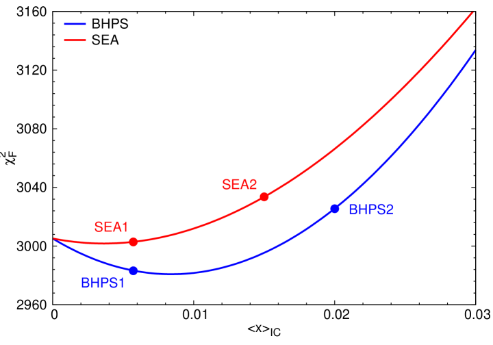
Figure 1 shows the results of the two IC series. We plot here the global chi-square function, , versus the intrinsic charm content, , for the two models of intrinsic charm. The BHPS model is shown in blue; The SEA model is shown in red. The function , which is called in Ref. ct10nn , includes the treatment of correlated systematic errors. The parabolic curves are determined from fits with many values of . Two exemplary fits for each model are shown as dots. They have and for the BHPS models; and and for the SEA models. These 4 examples will be used in the subsequent discussion.
Figure 1 provides a first step toward setting upper limits on the intrinsic charm. As increases, the goodness-of-fit to the global data set decreases, and at some point we judge that the data has ruled out the theory; this point could define a maximum acceptable value of . However, we know from experience that relying only on the value of is not always the best measure of the goodness-of-fit. For example, there may be PDFs with small global , but for which one or a few individual data sets are very poorly fit, balanced by especially good fits to other data sets. Furthermore, in the global , a particular experiment that is very sensitive to a fit parameter, but has a small number of data points will be relatively underweighted compared to other data sets that are less sensitive, but which have more data points. Thus, in order that the PDFs agree to a reasonable degree with all the individual data sets, we must also look at the values from individual experiments, not just the overall sum of the values.
To obtain a measure of the goodness-of-fit that includes the separate values of individual experiments, we introduce a “Tier-2 penalty” for each experiment . This measures the goodness-of-fit for that experiment; a large value means that the experiment is not consistent with the theory. ( is not simply , but they are related. is designed to increase more rapidly than when moves beyond the 90% confidence level. Additional details are given in the Appendix.)
The dotted curves in Figure 2 show versus for the two models of IC. Our usual choice for the “tolerance” of a PDF fit is
| (5) |
That is, a set of PDFs with is deemed to be such a poor fit to the data that it is ruled out (at the 90% confidence level). From Fig. 2 we see that in the present study, the contribution turns on and rises very sharply with , thus determining the upper limits on IC. The sharp increase in slope arises when one or more experiment becomes poorly fit as the charm momentum fraction increases. As we shall see and discuss in more detail in section III, the dominant constraint on the SEA model is from the combined HERA charm production measurements; however, the main constraints on the BHPS model come from several measurements, but not the HERA charm production experiments. We conclude that the upper limits on , at the 90% C.L., are:
Note that the four example PDFs are all within these limits. The global data does not rule out BHPS2 (which has ), nor SEA2 (which has ). However, these are close to the upper limits for , and can be taken as representative PDF models with amounts of IC near the largest acceptable value.
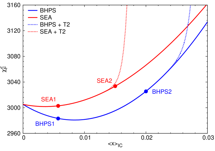
Figures 1 and 2 show that is disfavored for the SEA model, while the BHPS model allows a larger charm content, up to about . Furthermore, the BHPS model provides a value of that is lower than that of the standard CT10 PDFs for . The BHPS model with gives the best fit to the global data set. However, the small decrease is really not significant enough to herald the discovery of intrinsic charm. In the rest of the paper we shall focus on the four IC models marked as dots in Figs. 1 and 2, labelled as SEA1, SEA2, BHPS1 and BHPS2. The fraction of intrinsic charm component for each model is 0.57%, 1.5%, 0.57% and 2%, respectively, cf. Table 2.
The result in Fig. 1 is rather different from the corresponding result from our earlier NLO CTEQ6.5 study plt . The order of magnitude of the dependence of on is comparable to the earlier study. However, the behaviors of the BHPS model and the SEA model are reversed. In the current NNLO study, we find , leading to a larger upper limit on for the BHPS model. In the older NLO study the inequality was the reverse. Because of the advances in both theory and data, listed above, we trust that the current results are more realistic regarding the issue of intrinsic charm.
More extensive comparisons between theory and experiment are given in Section 3, while a discussion of the correlation of these fits with the value of the charm mass is deferred to Section 5.
II.1 The charm quark PDF
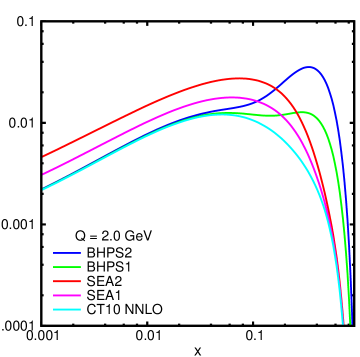
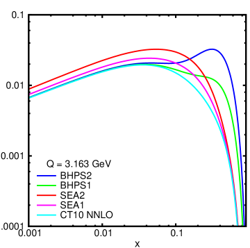
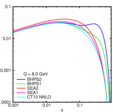
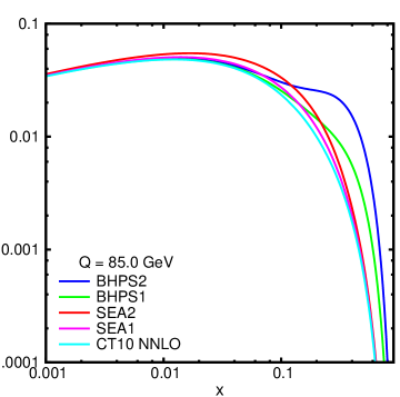
Figure 3 shows the charm quark PDF for five cases. In each panel, the function is shown for the BHPS1, BHPS2, SEA1, SEA2 and CT10 PDFs. The four panels correspond to four values of : . CT10 has no IC; . But the charm distribution evolves rapidly from to 2 GeV. For GeV and , the CT10 charm PDF is comparable to the IC models.
The BHPS model has a “valence-like” charm distribution at . So for small , the charm density with is significantly larger than our standard CT10 charm PDF. Even for as large as 85 GeV, is still notably larger for the BHPS model than for CT10, for large . On the other hand, for small , say , the BHPS model and CT10 charm densities are approximately equal for GeV. Because the IC in this model is concentrated at large , the resulting PDFs can fit most data comparably well as CT10, as long as is not too large; cf. Section 3.
The SEA model has a “sea-like” charm distribution at . There is a large density at for small and intermediate ranges, say . The charm PDF evolves rapidly from to 2 GeV, but nevertheless continues to be notably larger than CT10 at small , even for as large as 8 GeV. Because of this large charm density at low , the SEA model has a more difficult time fitting the combined HERA charm data than CT10, or than the BPHS model for equal values of ; cf. Section 3.
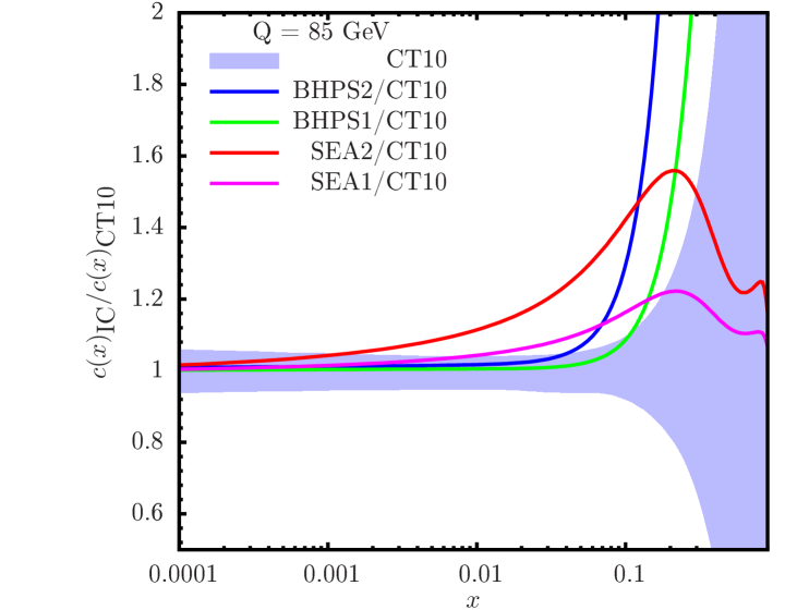
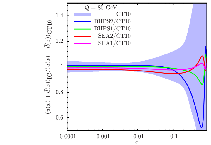
To emphasize the differences between the models, relevant to LHC experiments, Figure 4 compares for the four examples of the BHPS and SEA models, at the large momentum scale . For each case the ratio is plotted as a function of . The shaded region is the uncertainty band for the charm distribution of CT10 at . Note that the charm distributions with IC are allowed to be outside the uncertainty band of CT10, since CT10 was created with the constraint that the charm PDF was radiatively generated.
Putting intrinsic charm into the and distributions will, of course, directly affect predictions involving charm quarks in the initial state. But there will also be indirect effects. Because of the momentum sum rule, other parton distributions must change to balance the change in the charm distribution. Therefore we should also look at other parton distributions in the PDF sets with intrinsic charm.
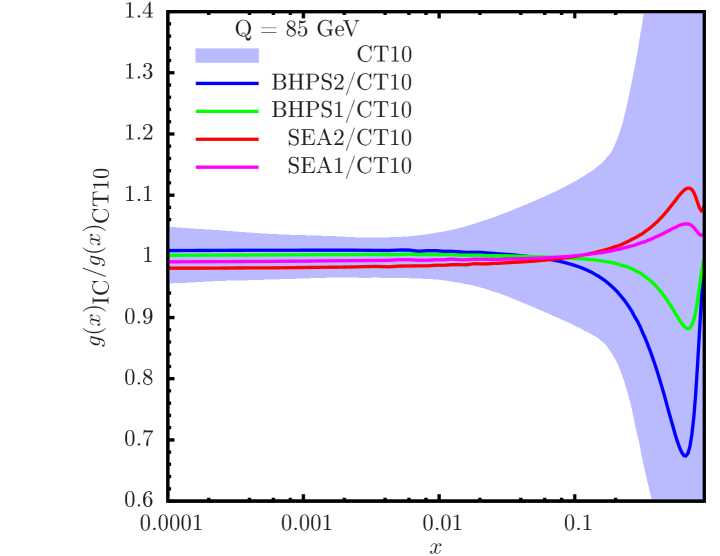
Figure 5 shows the gluon PDF for the same four examples of the BHPS and SEA models as in Fig. 4, again plotting the ratio to CT10, for the momentum scale . Figure 6 shows the same for the quark PDF. The shaded regions show the uncertainty bands for CT10. We note that for the BHPS model, the presence of intrinsic charm pulls momentum from the gluon and the quark at large ; whereas for the SEA model, the presence of IC pulls momentum from the quark at small . This will affect LHC predictions in interesting ways; cf. Section 4. Before concluding this section, we note that each IC fit is a central fit, with a different assumption on the intrinsic charm distribution at the scale . Hence, if we would compute eigenvector (Hessian) uncertainties for these IC fits, we would obtain an uncertainty range that expands on the CT10 uncertainty range for these gluon and quark distributions.
III Experimental data sets and intrinsic charm
The experimental data sets included in the global analysis that led to the results of Section II are listed in Table 1. With a few exceptions, they are the same as the data used in the standard CT10 fit ct10nn . We note that the CT10 PDFs were fitted to the individual data sets from both H1 and ZEUS Collaborations. As shown in Table 1, in this study we have replaced those individual data sets by the combined H1 and ZEUS reduced cross section data (called Data Set 147) for charm production at HERA HERAX0c .
The impact of an intrinsic charm component on the fit to the different data sets can be visualized in several different ways. In Table 1, we have listed the number of data points, , for each experiment, as well as the for the CT10 fit, the BHPS2 fit, and the SEA2 fit, which have charm momentum fractions () of 2% and 1.5%, respectively. The change in in the last two columns from the CT10 fit indicates which data sets are in conflict with a large intrinsic charm content.
| ID | Experimental data set | CT10 | BHPS(0.020) | SEA(0.015) | |
| 101 | BCDMS Benvenuti:1989rh | 339 | 1.158 | 1.087 | 1.220 |
| 102 | BCDMS Benvenuti:1989fm | 251 | 1.157 | 1.119 | 1.187 |
| 103 | NMC Arneodo:1996qe | 201 | 1.656 | 1.668 | 1.582 |
| 104 | NMC Arneodo:1996qe | 123 | 1.210 | 1.311 | 1.207 |
| 108 | CDHSW Berge:1989hr | 85 | 0.832 | 0.833 | 0.781 |
| 109 | CDHSW Berge:1989hr | 96 | 0.809 | 0.867 | 0.810 |
| 110 | CCFR Yang:2000ju | 69 | 0.989 | 1.105 | 0.943 |
| 111 | CCFR Seligman:1997mc | 86 | 0.387 | 0.416 | 0.417 |
| 124 | NuTeV di- SIDIS Mason:2006qa | 38 | 0.781 | 0.836 | 0.745 |
| 125 | NuTeV di- SIDIS Mason:2006qa | 33 | 0.852 | 0.905 | 0.864 |
| 126 | CCFR di- SIDIS Goncharov:2001qe | 40 | 1.195 | 1.204 | 1.145 |
| 127 | CCFR di- SIDIS Goncharov:2001qe | 38 | 0.692 | 0.728 | 0.655 |
| 147 | HERA charm production HERAX0c | 47 | 1.187 | 1.185 | 1.424 |
| 159 | Combined HERA1 DIS :2009wt | 579 | 1.068 | 1.086 | 1.059 |
| 201 | E605 DY process Moreno:1990sf | 119 | 0.804 | 0.845 | 0.796 |
| 203 | E866 DY process Towell:2001nh | 15 | 0.658 | 0.789 | 0.718 |
| 204 | E866 DY process Webb:2003ps | 184 | 1.271 | 1.286 | 1.277 |
| 225 | CDF Run-1 charge asymmetry Abe:1996us | 11 | 1.292 | 1.191 | 1.285 |
| 227 | CDF Run-2 charge asymmetry Acosta:2005ud | 11 | 0.978 | 0.995 | 0.978 |
| 231 | D0Run-2 charge asymmetry Abazov:2008qv | 12 | 1.928 | 2.006 | 1.972 |
| 234 | D0Run-2 charge asymmetry Abazov:2007pm | 9 | 1.501 | 1.709 | 1.371 |
| 260 | D0Run-2 Z rapidity dist. Abazov:2006gs | 28 | 0.580 | 0.551 | 0.550 |
| 261 | CDF Run-2 Z rapidity dist. Aaltonen:2010zza | 29 | 1.586 | 1.466 | 1.535 |
| 504 | CDF Run-2 inclusive jet Aaltonen:2008eq | 72 | 1.398 | 1.431 | 1.311 |
| 514 | D0Run-2 inclusive jet :2008hua | 110 | 1.044 | 0.950 | 1.012 |
| Totals: |
One especially interesting data set for this paper is the combined H1 and ZEUS data for charm production in deep-inelastic collisions at HERA HERAX0c . This is Data Set 147 in Table 1. Charmed particles can be produced in two ways in an collision: the charm-excitation process , and the charm-creation process . These are combined consistently in the calculations using the prescription introduced by ACOT acot . However, in the presence of intrinsic charm, the former process becomes particularly important, since it is directly proportional to the and component of the proton. Thus, one would expect data set 147 to be particularly sensitive to intrinsic charm. In addition, this set of combined H1 and ZEUS data has smaller systematic errors than the separate data sets, which were used in our previous analysis plt . Therefore we are interested to assess the influence of this newly available high-precision combined data.
Figure 7 shows a comparison of the H1 and ZEUS combined data on charm production with the theory predictions using IC parton distributions. The agreement between data and theory for BHPS2 is satisfactory, and almost the same as for the CT10 PDFs. On the other hand, we see systematic differences between the data and SEA2, whose prediction is consistently higher than the data over the full range of and . Table 2 lists the values of for CT10 and our four representative IC models with different amounts of IC. In general the models with sea-like intrinsic charm do worse than the standard fit or the fits with the BHPS model with valence-like intrinsic charm. The sea-like models have more charm at low values of , which is disfavored by this HERA data with small . We note, however, that the increase in for SEA2 is only about 13 units, to be compared to 47 data points.
| Model | ||
|---|---|---|
| CT10 | 0% | 55.75 |
| BHPS1 | 0.57% | 55.78 |
| BHPS2 | 2% | 56.29 |
| SEA1 | 0.57% | 57.60 |
| SEA2 | 1.5% | 68.50 |
The impact of intrinsic charm on the other data sets in Table 1 is not so obvious as for the charm production set 147. Some data sets favor the SEA models, while other data sets favor the BHPS models, while still others disfavor both. One other data set to note in particular is data set 101, which is the BCDMS data. Although the decrease in for BHPS2, and the increase in for SEA2, are not obviously significant, the large number of data points ensures that these have an affect on the total . In this case the BHPS2 fit has reduced by 24 units compared to CT10, while the SEA2 fit has increased by 21 units. The net effect is that the full combination of all data sets to the total disfavors the SEA model of intrinsic charm more than the BHPS model of intrinsic charm, for a given intrinsic charm momentum fraction, as seen in Fig. 1.
III.1 Spartyness: an equivalent gaussian variable
From the discussion in the last paragraph, we can see that the naive use of total as the discriminating variable may overweight data sets with large numbers of points, even if the correlation with the fitting parameter is not very significant. It was for this reason that the Tier-2 penalty was added to in the global fitting program. The Tier-2 penalty makes use of a variable , which we call spartyness, which gives a measure of the goodness-of-fit for each of the individual data sets. It is defined precisely in the Appendix.
In words, we obtain the spartyness for a particular data set by mapping its value, assumed to obey a chi-square probability distribution, onto the variable which has the same probability but for a standard Gaussian distribution. (cf. Appendix)
The values of can then be interpreted in terms of probabilities in a normal distribution. Fits with between -1 and 1 are accepted as reasonable, within the errors. Fits with are considered poor fits. Fits with actually fit the data much better than one would expect from normal statistical analysis; i.e., they have anomalously small residuals, presumably because the true experimental errors are smaller than the published values.
Figure 8 shows for all 25 individual data sets, for the two models of IC, as a function of . The BHPS model is shown above, and The SEA model is shown below. To focus on the data sets which are most affected by intrinsic charm, we select out just these in Figure 9.
For the BHPS model we see that several of the data sets have a slow increase in spartyness with momentum fraction , while data set 101 (BCDMS ) has a significant decrease in spartyness for small , and then levels off for larger . This is consistent with the results of Fig. 1 which showed that the BHPS models for were actually slightly favored over zero intrinsic charm, but increasing further decreased the overall goodness of fit for the BHPS model. The increase in or seen in Figs. 1 or 2 at for the BHPS model can be attributed to several experiments: ID 104 (NMC ), ID 110 (CCFR ) and ID 504 (CDF Run-2 inclusive jets); note that increases for these experiments in Fig. 9. The abrupt increase of at comes from experiment ID 110.
In contrast, the SEA model shows a strong increase in spartyness as increases for several experiments, in particular for the HERA combined charm experiment ID 147. (The CDHSW measurement of , experiment ID 108, shows a strong decrease in spartyness; but we note that that experiment is already anomalously well-fit, even for no intrinsic charm.) Again, this is consistent with the rapid rise of versus in Figure 1 at ; but Figure 8 is more informative, because it shows which experiments are responsible for the rapid rise in , i.e., which experiments conflict with the large IC. In fact, it is the HERA combined charm experiment 147 that gives the dominant contribution to the Tier-2 penalty for the SEA model, and determines the limit on charm momentum fraction from Fig. 2.
Overall, we can use the spartyness plots to understand which data sets can or cannot be fit by a particular model of intrinsic charm. For instance, the BHPS model actually gives a better global fit for because that significantly lowers the spartyness of the BCDMS data set 101; at the same time it does not conflict with HERA inclusive charm data set 147. Evidently, intrinsic charm at large at does not conflict with charm production at HERA (low and large ), while it can improve the agreement with the BCDMS data. On the other hand any increase in the SEA model intrinsic charm (predominantly low charm) worsens the fit to both data sets 101 and 147.
IV Predictions for the LHC
The inclusion of intrinsic charm changes the charm quark distributions at high values significantly, as well as affects the gluon and other quark PDFs through the PDF correlations in the global fit as shown in Section II. Thus it may have impact on collider observables ct66 . For example, in Figs. 10-13 we show the predictions of the NNLO total cross sections for and boson production, Higgs boson production through gluon fusion, and top quark pair production at the LHC at and 14 TeV. The NNLO cross sections for and boson production are computed with FEWZ2.1 fewz1 ; fewz2 . The NNLO cross sections for Higgs boson and top quark pair production are obtained from iHix1.3 ihixs and Top++2.0 toppp1 ; toppp2 , with , and the QCD scales set to the corresponding mass values. For each pair of total cross sections, we show the central predictions from CT10 with the 90% C.L. PDF tolerance ellipse as well as predictions from the four examples with intrinsic charm.
In Figs. 10-13, generally the predictions from the chosen IC models differ from the central predictions of CT10 by less than 2%, which is smaller than the PDF uncertainties of CT10 but may not be negligible for precise predictions for the LHC. For the SEA models, the cross sections at the LHC are almost uniformly smaller, due to the reduction in momentum fraction remaining for the other non-charm partons. The only exception is production through the process , which benefits from the increased distribution. The production of Higgs bosons and top quark pairs, in particular, are reduced for nonzero IC SEA, due to the reduction in gluons and light sea quarks in the relevant regions of and , as seen previously in Figs. 5 and 6.
For the BHPS models, the situation is more complicated, since the gluon and light sea quark PDFs are increased in the region in the BHPS models. In this case the production of and (independent of sign) are increased and the production of top quark pairs is decreased by an increase of IC in the BHPS models. The production of Higgs bosons is fairly insensitive to the amount of IC for the BHPS model. Also it is interesting to see from Figs. 10, 11 and 13 that the predictions from the BHPS models follow similar (anti) correlations as CT10 since they distribute along the diagonal direction of the ellipse, in distinction to the SEA models.
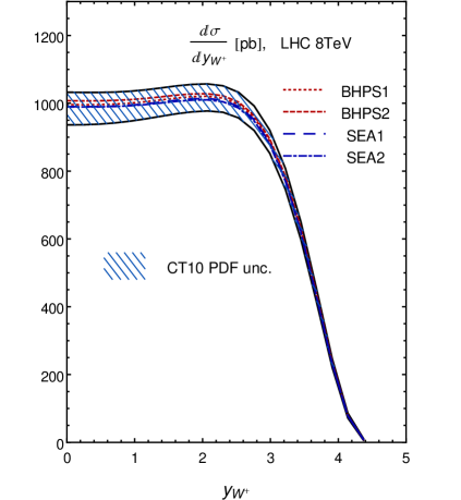
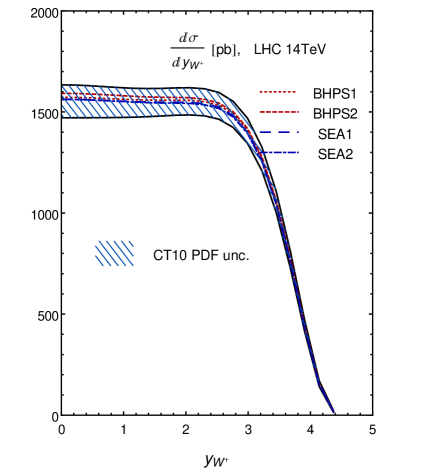
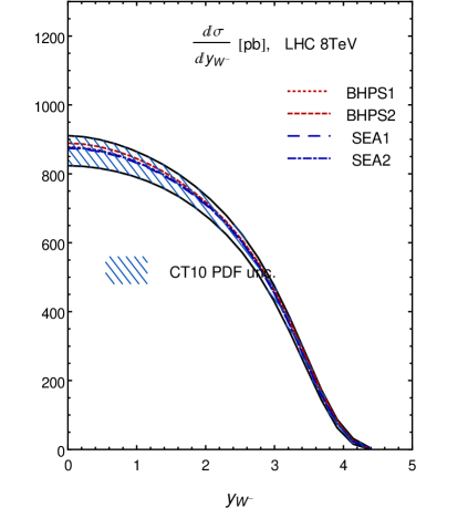
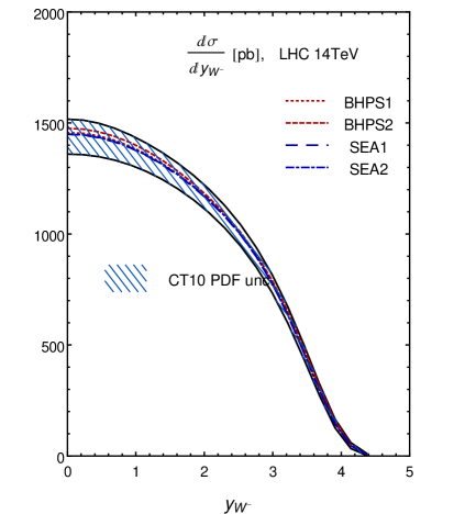
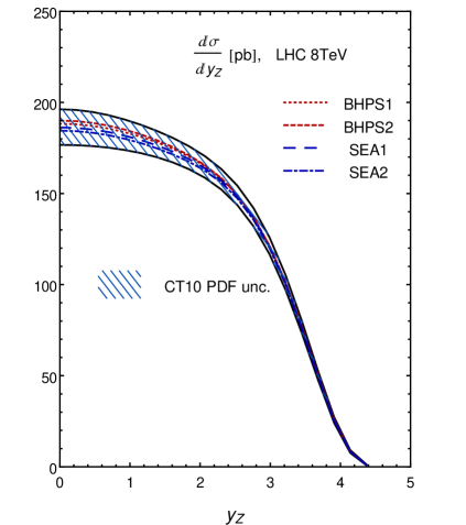
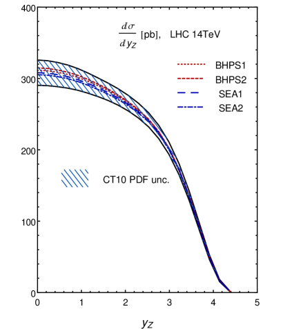
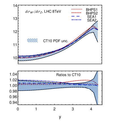
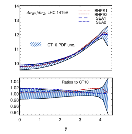
We can also check the effects of the IC on the rapidity distribution of the vector boson production. Charm quark contributions there have different shapes compared to the light quarks depending on the momentum profile of the charm quark of the IC models. Figs. 14-16 give the NNLO predictions of the rapidity distributions of and Z boson productions from CT10 and the four IC models. They are calculated with the program Vrap0.9 vrap , and both the renormalization and factorization scales are chosen to be the mass of the vector boson. The differences are small among four IC models, and their predictions are all within the CT10 PDF uncertainties. In Fig. 17 we further plot the ratios of the rapidity distribution, , which presumably are more sensitive to the charm quark contributions due to the cancellations of the uncertainties from light quark contributions. This is evident from comparing the size of error band induced by the PDF uncertainty in Figs. 14-16 to that in Fig. 17. We can see that in the small or intermediate rapidity region the predictions of SEA2 lie outdide the CT10 PDF uncertainties, similar to that for BHPS2 in the large rapidity region.
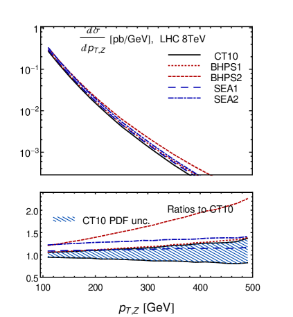
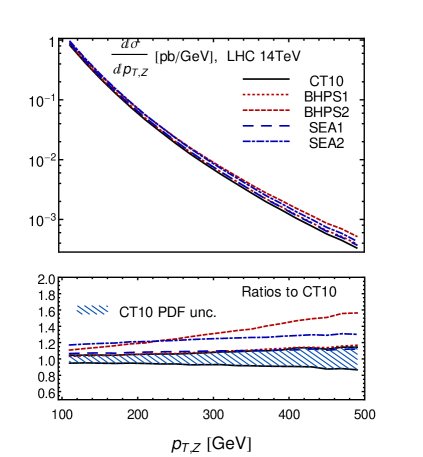
As already pointed out in our previous IC study plt , and recently in Refs. zq1 ; zq2 , the partonic process is directly sensitive to the initial state charm distribution, although precision measurements could be experimentally challenging at the LHC. Figure 18 shows predictions of the differential cross sections of an on-shell boson production in association with a charm quark at the LHC from CT10 and the IC models. The matrix element calculations of the process are only available up to NLO in QCD zq3 and are implemented in program MCFM mcfm . We simply convolute them with our NNLO PDFs in order to show the relative changes of the cross sections in the presence of IC. Figure 18 gives the transverse momentum distribution of the boson with kinematic cuts of , and applied on the charm quark jet using the anti- algorithm with the radius parameter . In this calculation, both the renormalization and factorization scales are chosen to be the scale sum of the transverse momenta of final state particles. We have checked that in the large region, the theoretical uncertainty induced by varying these scales simultaneously by a factor of 2 is much smaller than the error induced by the CT10 error PDFs.
We can clearly see that in the large region, predictions from the fits with IC models deviate sigificantly from CT10 as a direct result of the charm distribution changes shown in Fig. 18. Thus, it shows a potential for discriminating the possible IC models. In particular, at large values of it is very sensitive to the presence of IC in the BHPS models, since they have a large enhancement at large . However, the cross sections are small, and there are further suppressions from the decay branching ratios of the boson, as well as the charm quark jet-tagging efficiency. A detailed study of the feasibility of this process at the LHC is needed, but it is beyond the scope of the current work.
V Correlations between the charm mass and intrinsic charm
The curves in Fig. 3 show that the charm distribution in the SEA model is very similar in shape to the charm distribution of CT10 with no IC. It mostly differs in overall normalization. This then begs the question whether it can be distinguished from some other physics that may produce more radiation, such as a change in the charm quark mass, . In this section we investigate the correlation between and IC in the SEA model.
A lighter charm quark mass could mimic the effects of intrinsic charm, because with a smaller mass, the charm PDF turns on sooner, resulting in more charm at a given value of . Conversely, a larger value of the charm mass would result in a smaller charm content at a given value of , which could then be made up with some intrinsic charm. This possibility is intriguing because the standard value of the charm mass GeV, which was used in the CT10 analysis ct10nn and was shown to be favored by the global analysis data smucharm , is smaller than the world average given by the Particle Data Group (PDG) pdg , which was obtained using a mostly orthogonal set of data. The PDG gives a world average value of GeV, which translates into pole mass values of GeV and GeV at one-loop and two-loop conversions, respectively. Thus, one may wonder if the lower value of used in the global analysis is actually hiding some evidence for intrinsic charm.
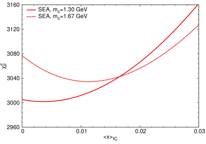
Rather than performing a combined fit of and IC, we shall just demonstrate the effect by re-running the analysis of section II, using the larger value of GeV. We emphasize that we are not advocating this large value of the charm mass, but are just using it to observe the correlation between fits of the charm mass and intrinsic charm. In Fig. 19 we plot the results of the global fitting for versus the intrinsic charm content, , for the SEA model, both for our standard charm mass GeV and for the larger value of GeV. We keep the same initial scale for the light partons, GeV, for both choices of . As seen previously, the dependence of on for GeV is quite flat for small charm content and then begins to rise. The curve looks like a quadratic function with a minimum close to . This is consistent with the fact the GeV is near the best fit of the charm mass with zero IC to the global analysis data. On the other hand, for GeV, the begins at a higher value for zero IC and then noticeably decreases to a minimum at around . Thus, if a larger value of the charm mass could be decisively shown to be required, then the global analysis would prefer nonzero IC, even for the SEA model, although this preference is not currently statistically significant.
We note, however, that the overall value of is still worse for GeV and than for GeV with zero intrinsic charm. We investigate this further in Fig. 20, where we compare the “spartyness” as a function of for the same set of experiments that were sensitive to the SEA model in Fig. 9 for GeV. The main thing to note here is that the spartyness for data set 147, combined charm production at HERA, is significantly worse for GeV than for GeV. For GeV and zero IC, the spartyness of data set 147 is more than 5, which indicates a very poor fit to the data. Increasing the IC content makes the fit better for this charm mass, but the spartyness is still a good bit higher than that with GeV and no IC. In addition, the fit to the combined HERA1 DIS data set 159 worsens as the charm momentum fraction increases for the SEA model with GeV.
VI Conclusions
The hypothesis of intrinsic charm (IC) is a long-standing question in high-energy physics, combining QCD theory (both perturbative and nonperturbative) and phenomenology.bhps The purpose of this paper is to reassess the theory based on up-to-date global analysis of QCD at the NNLO approximation.
The final conclusion of this work is that the wide range of short-distance processes that are commonly used in global analysis can be described accurately without an IC component of the proton; however, they do not rule out a small IC component. Quantitatively, we can construct PDFs that are acceptable fits to the global data (acceptable within the 90% C.L.) with for a sea-like IC in the SEA model at ; or with for a valence-like IC (i.e., concentrated at large ) in the BHPS model, cf. Fig. 2.
The HERA combined data on inclusive charm production in ep deep-inelastic scattering is particularly important. It constrains the SEA model more strongly than other data. On the other hand, it neither constrains nor favors the large- IC of the BHPS model.
We also investigated the correlation between IC content and the value of the charm quark mass in the global fits. We found that a larger value of was better fit with larger amounts of intrinsic charm, even for the SEA model. (The best fit for GeV required about for the SEA model.) However, the HERA combined data on inclusive charm production has a significant tension with larger values of the , which is only somewhat alleviated by including nonzero IC. Thus, the overall best fit to the data with the SEA model still appears be with the smaller charm quark mass GeV and small or zero IC.
Predictions for LHC measurements, based on the IC PDFs, are interesting. The figures in Sec. IV show that the IC models with largest allowed IC, are right up against the uncertainty limits for the CT10 PDFs. In other words, the PDF uncertainties are just as large as the IC effects. Global analysis cannot say more about IC until the PDFs are more accurately determined. (Special interactions, especially sensitive to the charm quark but not used in global analysis, might be able to say more.) But more accurate measurements at the LHC will reduce the PDF uncertainties. The results of Sec. IV show that new LHC results will impact the limit on intrinsic charm. Or, if intrinsic charm is real then the results of Sec. IV indicate that it will show up as a discrepancy between theory and data in some common LHC measurements. For example, Fig. 14 shows that the BHPS models can strongly modify the distribution in associated production of boson and charm jet.
Some recent research regarding intrinsic charm has focused on inclusive charm production at the LHC or Tevatron lhccharm ; Kniehl09 ; Bugaev10 ; Lykasov12 , or on associated production of charm with a prompt photon Abazov09 ; Stavreva09 ; Stirling12 ; Lipatov12 ; Bednyakov13 . The IC PDFs constructed here can be used to make up-to-date predictions for those processes. This set of CT10 IC PDFs will be made available via an internet website.
Appendix: Spartyness: an equivalent gaussian variable
We introduce the variable , to simplify the comparison of data and theory for the many data sets in the global analysis. is the equivalent Gaussian variable, equivalent in likelihood to a given chi-square measure.444For a short nickname, we call the “spartyness”.
We could, of course, just use the individual values of as measures of the goodness-of-fit for the different data sets, e.g., as in Table 1. However, that variable has different meanings for different values of . For example, has a much different meaning than , although they have the same value. The chi-square probability for is 0.358; the probability for is 0.232. And the probability for is only 0.015. Different data sets in the global analysis have very different numbers of data ; so the meaning of different values of is not manifest.
The variable is designed to clarify the goodness of fit, by transforming the cumulative probability from the Chi-Square distribution (which can be misleading because it depends on ) to the normal distribution (which is more familiar).
The spartyness is a function of and . Let denote the -probability distribution function (PDF) for variables. Its cumulative distribution function (CDF) is
| (6) |
The definition of is
| (7) |
We find that this variable is very helpful in judging the goodness of fit for the individual experiments in the global analysis; cf. Section 3. The pure definition is not very convenient for computation. Therefore we use an accurate approximation for TLewis
| (8) | |||||
| (9) |
Ideally, the variable has an approximately Gaussian distribution with mean 0 and standard deviation 1. For a good fit to data, the value of should be roughly between -1 and 1. A fit with should be considered a poor fit. For a fit with , equivalent to , we might assume that the actual systematic errors are smaller than the values used in the calculation of .
In reality, the variable is unexpectedly large for some data sets, which are never fit very well in global analysis. Therefore, we do not judge the absolute values of , but rather the relative values—relative to the best global fit—when comparing different sets of PDFs. For example, in Figs. 8 and 9 we assume it is not the absolute value of for a chosen experiment that is relevant; but the change in the value as a function of , which informs about the sensitivity of the experiment to the amount of intrinsic charm.
The Tier-2 penalty.
When comparing the quality of agreement between theory and data, especially comparing alternative PDFs to a central fit, we impose additional penalties for large increases of . The penalty for experiment increases faster than as distance to the central fit increases, when the likelihood of data set goes below 10%. Then using to judge the goodness of fit, we can exclude test PDFs for which one or a few data sets do not respect the 90% confidence level. Technically, we define the Tier-2 penalty for experiment by , where the exponent is greater than 2. The Tier 2 penalties in this paper were calculated by arbitrarily taking to be 16. (We do not impose an added penalty on experiments with .)
The Tier-2 penalty is not used in finding the central fit, but it is used in constructing the error PDFs in the Hessian error analysis. That helps to avoid error PDFs that conflict (outside the 90% confident level) with individual data sets. We also use the Tier-2 penalty when estimating uncertainties of alternative PDFs in the manner of Figure 2. The simple requirement that the global must be less than some chosen “tolerance” is not adequate; we must assure that no individual experiment would definitively rule out the alternative PDFs.
Acknowledgments
We thank G. Salam for the useful discussions on the Hoppet program, and M. Guzzi and P. Nadolsky for discussions on the effect of charm mass to the global analysis. T.J. Hou thanks the hospitality of the Michigan State University where part of his work was done. This work was supported in part by the U.S. National Science Foundation under Grant No. PHY-0855561; by the U.S. DOE Early Career Research Award DE-SC0003870; and by the National Natural Science Foundation of China under the Grant No. 11165014.
References
- (1) Jun Gao, Marco Guzzi, Joey Huston, Hung-Liang Lai, Zhao Li, Pavel Nadolsky, Jon Pumplin, Daniel Stump, C.-P. Yuan, arXiv:1302.6246 [hep-ph].
- (2) S. Moch, J. A. M. Vermaseren and A. Vogt, Nucl. Phys. B688, 101 (2004); A. Vogt, S. Moch and J. A. M. Vermaseren, Nucl. Phys. B691, 129 (2004).
- (3) C. Anastasiou, L. J. Dixon, K. Melnikov and F. Petriello, Phys. Rev. Lett. 91, 182002 (2003); Rev. D69, 094008 (2004).
- (4) M. Aivazis, J. C. Collins, F. I. Olness, and W.-K. Tung, Phys. Rev. D50, 3102 (1994).
- (5) W. -K. Tung, S. Kretzer and C. Schmidt, J. Phys. G 28, 983 (2002) [hep-ph/0110247].
- (6) Marco Guzzi, Pavel M. Nadolsky, Hung-Liang Lai, C.-P. Yuan, Phys. Rev D86 053005 (2012), arXiv:1108.5112 [hep-ph].
- (7) M. Buza, Y. Matiounine, J. Smith and W. van Neerven, Eur. Phys J. C1, 301 (1998).
- (8) A. Chuvakin, J smith and W. van Neerven, Phys. Rev D61 096004 (2000).
- (9) R. Thorne and R. Roberts, Phys. Lett. B421, 3903 (1998).
- (10) S. Forte, E. Laenen, P. Nason and J. Rojo, Nucl. Phys. B834, 116 (2010).
- (11) R. D. Ball, V. Bertone, F. Cerutti, L. Del Debbio, S. Forte, A. Guffanti, J. I. Latorre, J. Rojo and M. Ubiali, Nucl. Phys. B849, 296 (2011).
- (12) J. Gao, M. Guzzi, and P. N. Nadolsky, arXiv:1304.494v1 [hep-ph].
- (13) K. G. Chetyrkin, J. H. Kuhn and M. Steinhauser, Comput. Phys. Commun. 133, 43 (2000) [hep-ph/0004189].
-
(14)
M. Buza, Y. Matiounine, J. Smith, R. Migneron and W. L. van Neerven,
Nucl. Phys. B 472, 611 (1996)
[hep-ph/9601302];
M. Buza, Y. Matiounine, J. Smith and W. L. van Neerven, Eur. Phys. J. C 1, 301 (1998) [hep-ph/9612398]. - (15) LHCb Collaboration (R. Aaij et al.), Nucl. Phys. B871, 1 (2013).
- (16) J. Pumplin, H.-L. Lai and W.-K. Tung, Phys. Rev. D75, 054029 (2007).
- (17) F. Aaron et. al., H1 and ZEUS Collaboration, JHEP 1001 (2010) 109.
- (18) H1 and ZEUS Collaborations, arXiv:1211.1182 [hep-ex].
- (19) S. J. Brodsky, P. Hoyer, C. Peterson, and N. Sakai, Phys. Lett. B93, 451 (1980).
- (20) G. P. Salam and J. Rojo, Comput. Phys. Commun. 180, 120 (2009) [arXiv:0804.3755 [hep-ph]].
- (21) A. C. Benvenuti et. al., BCDMS Collaboration, Phys. Lett. B223 (1989) 485.
- (22) A. C. Benvenuti et. al., BCDMS Collaboration, Phys. Lett. B237 (1990) 592.
- (23) M. Arneodo et. al., New Muon Collaboration, Nucl.Phys. B483 (1997) 3.
- (24) J. P. Berge et. al., CDHSW Collaboration, Z. Phys. C49 (1991) 187.
- (25) U.-K. Yang et. al., CCFR/NuTeV Collaboration, Phys.Rev.Lett. 86 (2001) 2742.
- (26) W. G. Seligman et. al., Phys. Rev. Lett. 79 (1997) 1213.
- (27) D. A. Mason, Ph.D. Thesis, FERMILAB-THESIS-2006-01,UMI-32-11223.
- (28) M. Goncharov et. al., NuTeV Collaboration, Phys.Rev. D64 (2001) 112006.
- (29) G. Moreno, et. al., E605 Collaboration, Phys.Rev. D43 (1991) 2815.
- (30) R. Towell et. al., FNAL E866/NuSea Collaboration, Phys.Rev. D64 (2001) 052002.
- (31) J. Webb et. al., NuSea Collaboration, Phys.Rev.Lett. (2003).
- (32) F. Abe et. al., CDF Collaboration, Phys.Rev.Lett. 77 (1996) 2616.
- (33) D. Acosta et. al., CDF Collaboration, Phys.Rev. D71 (2005) 051104.
- (34) V. Abazov et. al., D0 Collaboration, Phys.Rev.Lett. 101 (2008) 211801.
- (35) V. Abazov et. al., D0 Collaboration, Phys.Rev. D77 (2008) 011106.
- (36) V. Abazov et. al., D0 Collaboration, Phys.Lett. B658 (2008) 112.
- (37) T. A. Aaltonen et. al., CDF Collaboration, Phys.Lett. B692 (2010) 232.
- (38) T. Aaltonen et. al., CDF Collaboration, Phys.Rev. D78 (2008) 052006.
- (39) T. Affolder et. al., CDF Collaboration, Phys.Rev. D64 (2001) 032001.
- (40) V. Abazov et. al., D0 Collaboration, Phys.Rev.Lett. 101 (2008) 062001.
- (41) P. M. Nadolsky, H. -L. Lai, Q. -H. Cao, J. Huston, J. Pumplin, D. Stump, W. -K. Tung and C. -P. Yuan, Phys. Rev. D 78, 013004 (2008) [arXiv:0802.0007 [hep-ph]].
- (42) R. Gavin, Y. Li, F. Petriello and S. Quackenbush, Comput. Phys. Commun. 182, 2388 (2011) [arXiv:1011.3540 [hep-ph]].
- (43) R. Gavin, Y. Li, F. Petriello and S. Quackenbush, Comput. Phys. Commun. 184, 208 (2013) [arXiv:1201.5896 [hep-ph]].
- (44) C. Anastasiou, S. Buehler, F. Herzog and A. Lazopoulos, JHEP 1112, 058 (2011) [arXiv:1107.0683 [hep-ph]].
- (45) P. Baernreuther, M. Czakon and A. Mitov, Phys. Rev. Lett. 109, 132001 (2012) [arXiv:1204.5201 [hep-ph]].
- (46) M. Czakon, P. Fiedler and A. Mitov, arXiv:1303.6254 [hep-ph].
- (47) W. J. Stirling and E. Vryonidou, Phys. Rev. Lett. 109, 082002 (2012) [arXiv:1203.6781 [hep-ph]].
- (48) V. A. Bednyakov, M. A. Demichev, G. I. Lykasov, T. Stavreva and M. Stockton, arXiv:1305.3548 [hep-ph].
- (49) J. M. Campbell, R. K. Ellis, F. Maltoni and S. Willenbrock, Phys. Rev. D 69, 074021 (2004) [hep-ph/0312024].
- (50) J. M. Campbell and R. K. Ellis, Nucl. Phys. Proc. Suppl. 205-206, 10 (2010) [arXiv:1007.3492 [hep-ph]].
- (51) J. Beringer et. al. (Particle Data Group), Phys. Rev. D 86, 010001 (2012).
- (52) C. Anastasiou, L. J. Dixon, K. Melnikov and F. Petriello, Phys. Rev. D 69, 094008 (2004).
- (53) Bernd A. Kniehl, Gustav Kramer, Ingo Schienbein and Hubert Spiesberger, Phys. Rev. D79, 094009 (2009); Eur. Phys. J. C72, 2082 (2012).
- (54) E. V. Bugaev and P. A. Klimai, J. Phys. 37, 055004 (2010).
- (55) G. I. Lykasov, V. A. Bednyakov, A. F. Pikelner and N. I. Zimin, Euro. Phys. Lett. 99, 21002 (2012).
- (56) D0Collaboration (V. M. Abazov, et al.), Phys. Rev. Lett. 102, 192002 (2009); Phys. Lett. B719, 354 (2013).
- (57) T. P. Stavreva and J. F. Owens, Phys. Rev. D79, 054017 (2009).
- (58) W. J. Stirling and E. Vryonidou, Phys. Rev. KLett. 109, 082002 (2012).
- (59) A. V. Lipatov, M. A. Malyshev and N. P. Zotov, JHEP 1205, 104 (2012).
- (60) V. A. Bednyakov, M. A. Demichev, G. I. Lykasov, T. Stavreva and M. Stockton, arXiv:1305:3548 [hep-ph] (2013).
- (61) Toby Lewis, Austral. J. Statist. 30A, 160 (1988).