Helices in the wake of precipitation fronts

Abstract

A theoretical study of the emergence of helices in the wake of precipitation fronts is presented. The precipitation dynamics is described by the Cahn-Hilliard equation and the fronts are obtained by quenching the system into a linearly unstable state. Confining the process onto the surface of a cylinder and using the pulled-front formalism, our analytical calculations show that there are front solutions that propagate into the unstable state and leave behind a helical structure. We find that helical patterns emerge only if the radius of the cylinder $R$ is larger than a critical value $R>R_{c}$, in agreement with recent experiments.

I Introduction

Chiral patterns have been the subject of a large number of studies in natural sciences and engineering, as well as in the artistic domain Su-doublehelix ; Imai-chiral ; Gao-Zincoxid . The emergence of chirality at meso- and macro-scale is usually a complex process that may go along principally distinct routes. First, the chirality may be present in the microscopic building blocks and the symmetry is just transcribed to a higher level of spatial organization helicats . Second, achiral microscopic entities may assemble into chiral objects provided the process takes place in a chiral medium chiral-fibers . Finally, achiral microscopic units may self-organize into a chiral structure through symmetry breaking Sci-1982-Muller .

Our interest is in the symmetry breaking route, and this work is a follow-up to our recent studies Shibi2012 ; Shibi-Mat-Pack in which helical precipitation patterns were observed in the wake of moving reaction-diffusion fronts. In our experiments, we saw no chirality in the precipitation blocks at the microscale Shibi-Mat-Pack and, furthermore, the media, the precipitation dynamics, and the boundary conditions of the laboratory setup also lack chirality, thus we believe that the macroscopic patterns form through symmetry breaking. This view was also confirmed by simulations Shibi2012 that suggest that the helices emerge from a complex interplay among the unstable precipitation modes, the motion of the reaction front, and the noise in the system.

Although the simulations correctly describe the trends observed in experiments, one would also like to make analytical advances in at least some aspects of the above problem. In experiments using Liesegang-type setups (Fig.1), we measured the probability of the emergence of helices as a function of control parameters such as the concentrations of the inner and outer electrolytes, the temperature, and the radius $R$ of the test tube. A simple but remarkable feature of the observations (reproduced in simulations) is that the probability approaches zero at a critical radius $R_{c}$ below which no helical pattern forms. Our aim with this paper is to provide an explanation for the nonexistence of helical solutions below a critical radius $R_{c}$ using analytical calculations within the theoretical framework of Cahn-Hilliard precipitation dynamics CahnHill1958 which has been used successfully in simulations to interpret the experimental results Shibi2012 .

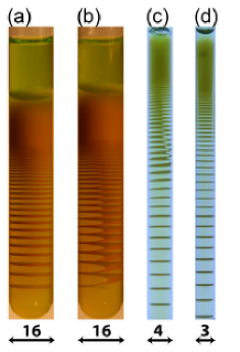
Figure 1: Liesegang experiments producing precipitation patterns in the form of (a) bands or (b) helices under identical external experimental conditions in tubes of radius $R=8$ mm (the numbers below the tubes are their diameters in mm). (c) Example when the radius is smaller ($R=2$ mm) and the helix becomes unstable as its pitch increases. (d) Only Liesegang bands form in tubes with radius $R\leq 1.5$ mm.

It should be noted that theoretical results about the absence of helical patterns below $R_{c}$ have been derived earlier on phenomenological grounds Polezhaev1991 ; Polezhaev1994 . Our work is based on similar logic in the sense that the conclusion is obtained by considering propagating helical waves evolving from an unstable state in precipitation dynamics. The differences lie in the use of a more transparent model of precipitation, and in the well defined approximation (pulled front formalism Saarloos2003 ) used for the analytic derivation of the bound on $R_{c}$.

We describe the experimental background and the results motivating our study in Sec.II, while the theoretical model and the pulled-front formalism are summarized in Sec.III. The theory is first applied (Sec.IV) to the emergence of regular Liesegang patterns (bands parallel to the front). Then helical solutions (bands tilted with respect to the front) are obtained (Sec.V), and the conditions for the existence of helical solutions are derived (Sec.VI). We conclude with discussions of more complex patterns and by reviewing the unsolved aspects of the problem (Sec.VII).

II Experiments

Precipitation patterns have captivated the imagination for a long time Henisch1991 and systematic studies of the so-called Liesegang bands (Fig.1) have been going on for more than a century Liesegang . In a typical Liesegang type experiment, a gel column soaked with a chemical reactant (called the inner electrolyte and denoted by $B$) is placed in a tube and another reactant (the outer electrolyte, denoted by $A$) is poured over the gel. The initial concentration of the outer electrolyte is chosen to be much larger than that of the inner electrolyte ($a_{0}\gg b_{0}$), thus a diffusive front moves into the gel where the reactions ($A+B\to\ldots\to C$) take place. For appropriate choice of reagents and initial concentrations, the final product $C$ emerges as a precipitate and the region of high concentrations of $C$ becomes visible as a pattern in the wake of the front.

The simplest patterns are the much studied Liesegang bands [see Fig.1(a)] which have been shown to obey a set of laws governing the distance between the consecutive bands, the width of the bands, and their time of appearance Henisch1991 ; MullerRoss2003 ; MathPack-1955 ; MatPack98 ; Liese-width1999 ; LieseRZ1999 . There are, however, complex precipitation patterns displaying curiosities such as bandsplitting, irregular banding, spirals, helices [see Fig.1(b,c)] and secondary- and revert patterns Sci-1982-Muller ; Shibi2012 ; Henisch1991 ; Mathur-revert ; Sultan-revert ; Volfi2007 ; Mofi2008 ; Lagzi-Grzy which are less readily explained. Frequently, they are just peculiarities of a given system, and some of them have problems with reproducibility. Our experiments Shibi2012 , however, proved that the emergence of helices is a robust phenomenon: They appear reproducibly with well defined probabilities for a given range of experimental parameters.

In our experiments, described in more detail in Shibi2012 ; exp-Lagzi , we used potassium chromate ($B\rm\equiv K_{2}CrO_{4}$) and copper chloride ($A\rm\equiv CuCl_{2}$) as the inner and outer electrolytes, respectively. The solid precipitate emerged from the reaction ${\rm Cu^{2+}+CrO_{4}^{2-}\to CuCrO_{4}\equiv}\,C$ which took place in a 1% agarose gel with the temperature kept constant ($T=22{\rm{}^{o}C}$). Below we display results for the following initial concentrations of the electrolytes: $\rm[Cu^{2+}]_{0}={\it a}_{0}=0.5M$ and $\rm[CrO_{4}^{2-}]_{0}={\it b}_{0}=0.01M$. The experiments were carried out for a set of test-tube radii in the range $\rm 1.5mm\leq{\it R}\leq 12.5mm$, and an estimate of the probability $P_{H}$ of the emergence of helices was obtained from ten experiments for each $R$ (Table 1).

Table 1: Probability of the emergence of helical pattern $P_{H}$ in experiments in which the test tube radius $R$ was the only parameter varied (see also Fig.1 in Shibi2012 ).

$R$ (mm)	1.5	2	3	4	5	6	7	8	9	10	12.5
$P_{H}$	0	0.1	0.1	0.2	0.1	0.2	0.3	0.7	0.2	0.2	0.1

As one can see from Table 1, the probability has a maximum around $R\approx 7-8$ mm, it decreases for large $R$ (due to the emergence of more complex structures such as double helices or chaotic patterns) as well as for small $R$, and it goes to zero at $R_{c}\approx 1.5$ mm. Below, we shall analytically derive the nonexistence of helices for $R<R_{c}$.

III Theory

Since the helical structures emerge at the macroscale and they can be viewed as slight variations of the usual Liesegang bands, we expect that they can also be analyzed within the framework of Cahn-Hilliard dynamics combined with a moving reaction front providing the precipitating material ModelB1999 . This approach has been successful in deriving the various laws describing the Liesegang bands, and it has helped in the understanding of how to control the bandspacing by external fields Guiding-field-07 ; Liese-2008 .

We shall actually further simplify the description, namely, the stage of the formation of the reaction product is replaced by an initial condition where the reaction product is homogeneously distributed with the concentration $c_{0}$. It is known that the diffusive reaction front leaves behind a homogeneous state of the reaction product MatPack98 ; LieseRZ1999 and helices usually form when a fast moving front prepares a relatively large region of the system in an unstable state Shibi2012 . We shall assume that this unstable state is the initial state for the precipitation dynamics studied by using the Cahn-Hilliard equation CahnHill1958 ; Halp-Hoh1977

$$\partial_{t}m=-\Delta(m-m^{3}+\Delta m)\,.$$ (1)

Here the field $m$ is a shifted and rescaled concentration with $m=\pm 1$ corresponding to the high- and low-concentration equilibrium values, and ${\cal F}(m)=-m^{2}/2+m^{4}/4+(\nabla m)^{2}/2$ is the free-energy density underlying the drive towards equilibrium. The coefficients in Eq.(1) are set to unity by choosing the length, time, and concentration scales appropriately.

Equation (1) is considered in a two-dimensional strip corresponding to the tube-in-tube experiments Shibi2012 where the helices emerge in a thin layer of gel in between two tubes of nearly equal radius. The cylinder can be cut and opened into a strip as shown in Fig.2 with the transformation implying that we have periodic boundary conditions across the strip. Initially, a homogeneous state $m(x,y,t=0)=m_{0}$ is prepared that is linearly unstable, i.e. the concentration is within the spinodal decomposition range, $|m_{0}|<1/\sqrt{3}$.

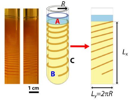
Figure 2: Liesegang type experiments with the precipitation patterns forming in the gel placed in between two tubes of nearly equal radius (Liesegang rings in the leftmost tube and a helix in the next one). On the right, a schematic drawing is displayed showing the transformation of the thin layer of gel in the tube-in-tube experiment into a two-dimensional strip.

Such an initial state is stationary, and so we add a small local perturbation $m_{0}\to m_{0}+\delta m(x,y,0)$ with $\delta m(x,y,0)$ restricted to the region $x\approx 0$, $0<y<L_{y}$. The perturbation develops into two precipitation fronts moving in the $\pm x$ direction and the question we pose is about the nature of patterns left behind the fronts. More precisely, we ask if a helix that is a striped pattern tilted with respect to the propagation direction is present among the solutions. In order to answer this question, we assume that the dynamics in the front region (where $\delta m=m-m_{0}\ll 1$) can be described by the linearized theory i.e. we assume that the front belongs to the pulled-front family Saarloos2003 . The theory of pulled fronts has been employed successfully to the $d=1$ Cahn-Hilliard equation Liu-Gold-89 ; Burki2007 ; Krekhov2009 . Below, we repeat (in a non-rigorous form) the main steps of the theory in order to clearly outline the assumptions needed for the generalization to the strip geometry of interest.

The first step in the theory of pulled fronts is the linearization of the equation in question, i.e. we write $m=m_{0}+\delta m$ and obtain from Eq.(1)

$$\partial_{t}\delta m=-\Delta(a+\Delta)\delta m$$ (2)

where $a=1-3m_{0}^{2}$ is a measure of the distance of the initial state from the spinodal ($a=0$). Equation (2) can be solved by Fourier transformation

$$\delta m(x,y,t)=\frac{1}{\sqrt{2\pi L_{y}}}\sum_{k_{y}}\int\limits_{-\infty}^{\infty}dk_{x}e^{i(k_{x}x+k_{y}y)}m_{\bf k}(t)$$ (3)

where ${\bf k}=(k_{x},k_{y})$ and, due to the periodic boundary conditions in the $y$ direction, we have $k_{y}=2\pi n/L_{y}$ with $n=0,\pm 1,...,\pm(L_{y}/2-1),L_{y}/2$. The Fourier components of the perturbation $m_{\bf k}$ evolve independently

$$m_{\bf k}(t)=e^{\omega_{\bf k}t}m_{\bf k}^{0}\,,$$ (4)

with $\omega_{\bf k}$ obtained by substituting (4) into (2)

$$\omega_{k}=ak^{2}-k^{4}\,,$$ (5)

where $k^{2}=k_{x}^{2}+k_{y}^{2}$.

In order to evaluate (3), the initial amplitudes $m_{\bf k}^{0}$ need to be specified. Since the initial perturbation is restricted to the $x\approx 0$ region, $m_{\bf k}^{0}$ is practically independent of $k_{x}$ and so $m_{\bf k}^{0}\approx m_{k_{y}}^{0}$. Thus we can write (3) in the form

$$\delta m(x,y,t)\approx\frac{1}{\sqrt{2\pi L_{y}}}\sum_{k_{y}}e^{ik_{y}y}m_{k_{y}}^{0}\int\limits_{-\infty}^{\infty}dk_{x}e^{{ik_{x}x}+\omega_{k}t}.$$ (6)

We shall now analyze the above expression term by term.

IV Liesegang-type patterns

It is clear that the $k_{y}=0$ term describes a one-dimensional pattern that is homogeneous in the $y$ direction. This brings us back to the one-dimensional case where, in the frame moving with the velocity $v_{0}$ of the front, we have

$$\delta m(v_{0}t+\xi,0,t)\sim\int\limits_{-\infty}^{\infty}dk_{x}e^{ik_{x}\xi}\exp{({ik_{x}v_{0}}+\omega_{k_{x}})t}\,.$$ (7)

A saddle-point evaluation of the $t\to\infty$ asymptote of the above integral, together with the requirement that $\delta m$ remains finite in the front region, leads to the basic equations of the theory of pulled fronts Saarloos2003

$$iv_{0}+\left.\frac{d\omega_{k_{x}}}{dk_{x}}\right|_{k_{x}^{*}}=0\quad;\quad{\rm Re}\,(ik_{x}^{*}v_{0}+\omega_{k_{x}^{*}})=0\;.$$ (8)

The above equations determine $v_{0}$ and $k_{x}^{*}=p_{0}+iq_{0}$ with $p_{0}$ and $q_{0}$ related to the characteristic wavenumber of the pattern in the comoving frame, and to the steepness of exponential decay of the front profile

$$\delta m(v_{0}t+\xi,0,t)$$

$$\sim\exp{\left[-q_{0}\xi+ip_{0}\xi+i(p_{0}v_{0}+{\rm Im}\,\omega_{k_{x}^{*}})t\right]}\,.$$ (9)

The values of $v_{0}$, $p_{0}$, and $q_{0}$ can be easily calculated from (8) and one obtains Saarloos2003

$$p_{0} = \frac{1}{2}\sqrt{\frac{\sqrt{7}+3}{2}}\,a^{1/2}\approx 0.840\,a^{1/2}\,,$$ (10)

$$q_{0} = \frac{1}{2}\sqrt{\frac{\sqrt{7}-1}{6}}\,a^{1/2}\approx 0.262\,a^{1/2}\,,$$ (11)

$$v_{0} = \frac{2}{3}\sqrt{\frac{7\sqrt{7}+17}{6}}\,a^{3/2}\approx 1.622\,a^{3/2}\,.$$ (12)

As we can see from the above results [Eqs.(10–12)], the spinodal ($a=0$) can be viewed as a critical point. Indeed, when approaching the spinodal ($a\to 0$), the characteristic length-scales ($\ell\sim 1/p_{0}\sim 1/q_{0}\sim a^{-1/2}$) and the characteristic time-scale ($\tau\sim\ell/v_{0}\sim a^{-2}$) diverge as in mean-field theories of critical phenomena.

The wavenumber of the pattern in the laboratory frame, $p^{st}_{0}$, is obtained by noting that, apart from the late stage coarsening process, the pattern becomes stationary in the laboratory frame. Thus $p^{st}_{0}$ is calculated by equating the frequency of precipitation bands leaving from the front region ($v_{0}p^{st}_{0}/2\pi$) to the frequency of the arrival of the perturbation maxima in the comoving frame $(p_{0}v_{0}+{\rm Im}\,\omega_{k_{x}^{*}})/2\pi$. As a result we find

$$p^{st}_{0}=p_{0}+\frac{{\rm Im}\,\omega_{k_{x}^{*}}}{v_{0}}=\frac{\sqrt{7}+1}{4}p_{0}\approx 0.766\,a^{1/2}\,.$$ (13)

Accordingly, the wavelength of the pattern (spacing of the precipitation bands) before the possible coarsening may take place is given by

$$\lambda_{0}^{st}=\frac{2\pi}{p^{st}_{0}}=\frac{16\pi}{3}\sqrt{\frac{19-7\sqrt{7}}{2}}a^{-1/2}\approx 8.206a^{-1/2}.$$ (14)

In some forms, the results embodied in Eqs.(10–13) have been derived in Refs. Saarloos2003 ; Liu-Gold-89 ; Burki2007 ; Guiding-field-07 ; Krekhov2009 ; Foard-Wagner-09 ; Foard-Wagner-11 ; Kopf-2012 where the front velocity and the characteristic length were calculated in various quench-related problems. The results were also used to describe enslaved phase separation dynamics Guiding-field-07 ; Foard-Wagner-09 ; Foard-Wagner-11 where the velocity of the front was slowly changing as prescribed by external fields. The logic in the present paper is similar to that used in the latter works. Namely, the wavelength of the pattern is identified as a changing local wavelength related to the velocity of the front and frozen in the wake of the front Guiding-field-07 . In case of Liesegang bands, this means that the front moves diffusively and slows down and, consequently, the distance between consecutive bands increases yielding the observed geometric series for the band positions Foard-Wagner-11 .

V Single-helix pattern

Next, we consider the case when the longest wave-length ($n=1$) transverse mode is excited only, i.e. the only nonzero amplitude in (6) is related to the mode $k_{y}=2\pi/L_{y}\equiv\kappa_{1}$. Thus, the initial perturbation takes the form

$$\delta m(x,y,t=0)\sim e^{i\kappa_{1}y}\int\limits_{-\infty}^{\infty}dk_{x}e^{{ik_{x}x}+\omega_{k}t}\,.$$ (15)

As in the $d=1$ case, the above expression is analyzed in the frame moving with the velocity $v_{1}$ of the front

$$\delta m(v_{1}t+\xi,y,t=0)\sim e^{i\kappa_{1}y}\int\limits_{-\infty}^{\infty}dk_{x}e^{ik_{x}\xi+{(ik_{x}v_{1}}+\omega_{k})t}\,,$$ (16)

where one expects a new value for the velocity front $v_{1}$ since $\omega_{k}$ now depends on $k^{2}=k_{x}^{2}+\kappa_{1}^{2}$. The equations to be solved remain the same (8) with $\omega_{k_{x}}$ replaced by $\omega_{k}$. Let us denote the solution of the equations by $k_{x}^{*}=p_{1}+iq_{1}$ where $p_{1}$ and $q_{1}$ depend not only on $a$ but also on $\kappa_{1}$. Then the perturbation in the comoving frame takes the form

$$\delta m(v_{1}t+\xi,y,t=0)$$

$$\sim\exp{[-q_{1}\xi+i(\kappa_{1}y+p_{1}\xi+{\rm Im}\omega_{k^{*}}t)]}\,.$$ (17)

with

$$p_{1} = \sqrt{\frac{\sqrt{(1-\theta)^{2}+6}+3(1-\theta)}{\sqrt{7}+3}}\,p_{0}$$ (18)

$$q_{1} = \sqrt{\frac{\sqrt{(1-\theta)^{2}+6}-(1-\theta)}{\sqrt{7}-1}}\,q_{0}$$ (19)

$$v_{1} = \frac{{\rm Re}\,\omega_{k^{*}}}{{\rm Im}\,k^{*}}$$

$$= \sqrt{\frac{[(1-\theta)^{2}+6]^{{3}/{2}}-(1-\theta)^{3}+18(1-\theta)}{7\sqrt{7}+17}}v_{0}$$

where the parameter $\theta$ is related to the width of the strip $L_{y}$ and the radius of the cylinder $(L_{y}=2\pi R)$ through

$$\theta=2\frac{\kappa_{1}^{2}}{a}=2\frac{(2\pi)^{2}}{L_{y}^{2}a}=\frac{2}{R^{2}a}\,.$$ (21)

It can be easily verified that, in the infinite width limit ($R\to\infty$ or $\theta\to 0$), we recover the parameters of the solution homogeneous in the $y$ direction [Eqs.(10)–(12)]. The scaled variables $p_{1}/p_{0}$, $q_{1}/q_{0}$ and $v_{1}/v_{0}$ are displayed in Fig. 3.

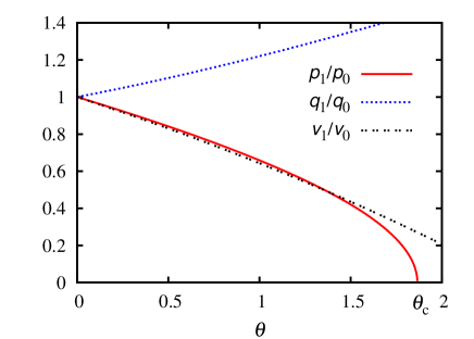
Figure 3: Characteristic wavenumbers $p_{1}$ and $q_{1}$ and the velocity $v_{1}$ of the propagating single helix pattern scaled by the corresponding homogeneous values $p_{0}$, $q_{0}$ and $v_{0}$. The parameter $\theta$ is inversely proportional to the square of the diameter of the tube (21). As can be seen, propagating helix solutions exist only for $\theta\leq\theta_{c}$ i.e. only for tubes with large enough diameter.

According to Eq.(16), the solution (18)–(V) is a wave of tilted precipitation bands propagating in the comoving frame. Due to the periodic boundary conditions in the transverse direction, the corresponding pattern on the cylindrical surface is a propagating helix. The pitch of the helix in the comoving frame is given by $\lambda_{1}=2\pi/p_{1}$ and, to obtain the pitch in the laboratory frame, $\lambda_{1}^{st}=2\pi/p_{1}^{st}$, we have to use again the stationarity of the pattern in the laboratory $p^{st}_{1}=p_{1}+{\rm Im}\,\omega_{k^{*}}/v_{1}$, resulting in

$$\lambda_{1}^{st}=\frac{2\pi}{p^{st}_{1}}=\frac{16\pi\sqrt{2}}{3}\frac{\sqrt{(1-\theta)^{2}+6}+2(1-\theta)}{[\sqrt{(1-\theta)^{2}+6}+3(1-\theta)]^{3/2}}a^{-1/2}.$$ (22)

We have thus found helix solutions with well defined propagation velocity and pitch determined by the parameter $a$ of the Cahn-Hilliard equation and by the width $L_{y}=2\pi R$ of the system.

VI Existence and relevance of the helix solutions

Examining $p_{1}$, $q_{1}$ and $v_{1}$ (18–V) reveals that the propagating helix solutions exist only for sufficiently small values of $\theta$. Indeed, as $\theta$ is increased from zero, the expressions under the square root in $p_{1}$ and $v_{1}$ become negative thus contradicting our assumptions that $p_{1}$, $q_{1}$ and $v_{1}$ are real. The smallest critical value of $\theta$ is obtained from the equation $p_{1}(\theta_{c})=0$ with the result

$$\theta_{c}=1+\sqrt{3}/2\approx 1.866\,.$$ (23)

Thus, we arrive at our main result, namely, helix solutions exist only if $\theta\leq\theta_{c}$. In terms of the radius $R$ of the test tubes, this inequality means that helices may emerge in a test tube only if $R$ exceeds a critical value

$$R\geq R_{c}=\sqrt{\frac{2}{\theta_{c}a}}\approx 1.035\,a^{-1/2}\,.$$ (24)

Estimating $R_{c}$ for a given system runs into the problem that $R_{c}$ is measured in unknown units since the details of mapping of the system onto the Cahn-Hilliard dynamics are usually lacking. We can go around this problem by obtaining the lengthscale from the results for the spacing of bands formed parallel with the front ($\theta=0$). The remarkable feature of this case is that the band spacing $\lambda_{0}^{st}$ is independent of $R$. Thus, using Eq.(14), we can write the inequality (24) in a simple form

$$R\geq R_{c}\approx 0.126\,\lambda_{0}^{st}\,.$$ (25)

To a good approximation, the above inequality means that helices can form if the diameter of the test tube is larger than 1/4 of the band spacing in identical experiments where bands were formed.

We can try now to carry out a straightforward comparison with the experiments and examine whether the inequality (25) is violated in cases in which no helices are observed. In the experiments, the diameters of the tubes $D=2R$ range in the interval 25 mm $\geq D\geq$ 3 mm. The radius is fixed for a given experiment, in contrast to the bandspacing $\lambda_{0}^{st}$ (or to the pitch $\lambda_{1}^{st}\approx\lambda_{0}^{st}$ of the helices) which changes within each pattern. In order to look for violation of the inequality (25), we took the largest values of $\lambda_{0}^{st}$ or $\lambda_{1}^{st}$ for each pattern and determined the corresponding smallest possible ratios $D/\lambda_{0}^{st}=u$ or $D/\lambda_{1}^{st}=u$. For the experiments displayed in Fig.1(a-d), we found $u_{a}>3.8$, $u_{b}>3.6$, $u_{c}>1.6$ and $u_{d}>1.2$. Thus the smallest $u$-s are significantly larger than 1/4 and the inequality (25) is not violated even in cases when helices are not formed. The conclusion remains the same if all the smallest $u$-s are calculated for the experiments and simulations studied in Shibi2012 . Clearly, the comparison with experiments works only at the qualitative level, namely, decreasing $R$ leads to the violation of the inequality and to the absence of helices, and this is in agreement with the observations.

We should emphasize that it is not surprising that we see only qualitative agreement. One should remember that the results, including the inequality (25), apply to propagating precipitation fronts. Thus, extending them to diffusive fronts such as the ones producing Liesegang bands or helices involves additional assumptions. First, the local velocity of the front is assumed to be identical to the linearly selected pulled front velocity. Second, the local wavelength of the pattern (bandspacing or pitch) emerging in the wake of the front is assumed to be frozen without any further coarsening. Using these two assumptions seems to work well when interpreting patterns formed in enslaved phase separation processes Guiding-field-07 ; Foard-Wagner-09 ; Foard-Wagner-11 , thus they can be viewed as reasonable assumptions. Naturally, one should suspect that while the mapping of the propagating front onto a diffusive one may leave the inequality (25) qualitatively valid, the constant $u$ in $2R>u\lambda_{0}^{st}$ (25) will be affected.

Unfortunately, there are additional problems when comparing the inequality (25) with Liesegang-type patterns. The pattern often evolves from a homogeneous precipitate called plug (see the upper part of the precipitation in Fig.1) with the initial bandspacing $\lambda_{0}^{st}$ being small and not always well resolved. Furthermore, the band-spacing grows exponentially, thus the $2R>\lambda_{0}^{st}/4$ rule (25) should always be violated for long enough tubes. Of course, the experimental tubes are finite and, as can be seen in the example shown in Fig.1(a), the $2R>\lambda_{0}^{st}/4$ rule is satisfied throughout the system. Thus, in this case one expects that there is no problem observing helical patterns, as indeed is the case [Fig.1(b)]. We have also seen examples when the band spacing is larger and the helical pattern becomes unstable as its pitch increases [Fig.1(c)], or when no helix forms at all [Fig.1(d)]. Whether this is the result of violating the inequality $D/\lambda>u$ with an effective (and presently unknown) $u$ remains an open question since coarsening and other nonlinear effects may always have unexpected effects on the stability of helices.

The trends in the experimental observations and in the related simulations Shibi2012 are, however, in agreement with the analytical result (25). Thus we feel that the assumptions required to extend the results of the pulled-front theory to diffusive fronts are valid and, consequently the inequality $D/\lambda>u$ is a relevant condition for helix formation in the wake of diffusive reaction fronts.

VII Discussions

One can easily verify that in addition to the propagating helix solutions (18)–(V), one can also find double-, triple-, and multiple-helix solutions. Indeed, one just repeats the helix calculation with $\kappa_{1}$ replaced by $\kappa_{n}=n^{2}\kappa_{1}$, where $n$ is the multiplicity of the helix. One can also verify, by noting that the effective $\theta$ for a helix with multiplicity $n$ is $n^{2}\theta$, that larger multiplicity results in smaller velocity and larger pitch. Furthermore, it also follows then that $\theta_{c}(n)=\theta_{c}/n^{2}$ and, consequently, the larger the multiplicity, the larger the threshold is for the tube diameter for the multiple-helix solution to exist.

In our experiments and simulations, we did observe single helices with large probability. Double helices had significant probabilities in large systems and at high noise levels (in the simulations). Although triple helices were also seen, their probability was negligible (could not be measured within the number of experiments and simulations carried out). Thus the modes we have been investigating do appear in the system and the outcome of their competitions seems to be determining the patterns emerging.

There are, of course, a number of problems to solve before the mode competition in the helix formation is fully understood. The stability of the helix solutions is clearly a relevant issue. One may expect that the helices are unstable in the linear regime (their velocity, e.g., is smaller than the velocity of the $\theta=0$ band solutions). As the experiments and simulations suggest, however, the helices are stabilized by the nonlinear effects. Thus, investigating the lifetime of the helices in the linear regime (as compared to the time the front moves the distance of the band spacing) may give an indication of how to start a calculation of $P_{H}$.

Clearly, the effect of noise is also important since the probability of the emergence of helices $P_{H}$ is negligible at small noise and it becomes of the order of 0.5 for appropriate noise amplitude. The origin of noise is not entirely clear. It may come as an initial-state noise left behind the fast moving reaction front. Another view (taken in Shibi2012 ) is that the inhomogeneities produced by the front are negligible, and the noise present in the precipitation process is the relevant effect. Finding the origin of noise would be essential in deciding whether the emergence of chirality is due to the initial-state effects or it is a symmetry breaking occurring in the course of the precipitation dynamics.

Another unclarified aspect of the problem is related to the boundary conditions. In the present paper, we assumed that the front is already at infinity, and we have to care only about the transverse boundary conditions (which are obviously periodic). In reality, the front is diffusive and, although it may move fast at the beginning, it can be seen to interact with the developing pattern Shibi2012 . Thus, the front may be relevant in the delicate interplay of the unstable modes and so, even if we would consider the front as a stationary wall, the boundary condition on it is highly nontrivial and needs to be explored.

In summary, we used analytical methods to understand a spatial constraint ($R>R_{c}$) in the formation of helices. Along the way, we also found that while the helices (and helicoids) are simple geometric objects, their formation through precipitation processes is a rather complex and intriguing problem, and much remains to be understood.

- (1) D. S. Su, Angew. Chem. Int. Edit. 50, 4747 (2011).
- (2) H. Imai, and Y. Oaki, Angew. Chem. Int. Edit. 43, 1363 (2004).
- (3) P. X. Gao, Y. Ding, W. J. Mai, W. L. Hughes, C. S. Lao, and Z. L. Wang, Science 309, 1700 (2005).
- (4) J. M. Lehn, A. Rigault, J. Siegel, J. Harrowfield, B. Chevrier, D. Moras, Proc. Natl. Acad. Sci. USA 84, 2565 (1987).
- (5) J. H. Jung, Y. Ono, K. Hanabusa, and S. Shinkai, J. Am. Chem. Soc., 122, 5008 (2000).
- (6) S. C. Müller, S. Kai, and J. Ross, Science 216, 635 (1982).
- (7) S. Thomas, I. Lagzi, F. Molnár Jr., and Z. Rácz, Phys. Rev. Lett. 110, 078303 (2013).
- (8) S. Thomas, F. Molnár Jr., Z. Rácz, and I. Lagzi, Chem. Phys. Lett. 577, 38 (2013).
- (9) J. W. Cahn and J. E. Hilliard, J. Chem. Phys. 28, 258 (1958); J. W. Cahn, Acta Metall. 9, 795 (1961).
- (10) D. S. Chernavskii, A. A. Polezhaev, and S. C. Müller, Physica D 54, 160 (1991).
- (11) A. A. Polezhaev and S. C. Müller, Chaos, 4 631 (1994).
- (12) W. van Saarloos, Phys. Rep. 386, 29 (2003).
- (13) H.K. Henisch, Periodic Precipitation, Pergamon Press, Oxford, 1991.
- (14) R. E. Liesegang, Naturwiss. Wochenschr. 11, 353 (1896).
- (15) S. C. Müller and J. Ross, J. Phys. Chem. A 107, 7997-8008, (2003).
- (16) R. Matalon and A. Packter, J. Colloid Sci. 10, 46 (1955); A. Packter, Kolloid Z. 142, 109 (1955).
- (17) T. Antal, M. Droz, J. Magnin, Z. Rácz, and M. Zrinyi, J. Chem. Phys. 109, 9479 (1998).
- (18) M. Droz, J. Magnin, and M. Zrinyi, J. Chem. Phys. 110, 9618 (1999).
- (19) Z. Rácz, Physica A 274, 50 (1999).
- (20) P. B. Mathur and S. Ghosh, Kolloid-Z. 159, 143 (1958).
- (21) T. Karam, H. El-Rassy, and R. Sultan J. Phys. Chem. A 115, 2994 (2011).
- (22) A. Volford, F. Izsák, M. Ripszám, and I. Lagzi, Langmuir 23, 961 (2007).
- (23) F. Molnár, F. Izsák, and I. Lagzi, Phys. Chem. Chem. Phys. 10, 2368 (2008).
- (24) S. K. Smoukov, I. Lagzi, and B. A. Grzybowski, J. Phys. Chem. Lett. 2, 345 (2011).
- (25) I. Lagzi, Langmuir 28 (2012) 3350.
- (26) T. Antal, M. Droz, J. Magnin, and Z. Rácz, Phys. Rev. Lett. 83, 2880 (1999).
- (27) T. Antal, I. Bena, M. Droz, K. Martens, and Z. Rácz, Phys. Rev. E76, 046203 (2007).
- (28) I. Bena, M. Droz, I. Lagzi, K. Martens, Z. Rácz, and A. Volford, Phys. Rev. Lett. 101, 075701 (2008).
- (29) The Cahn-Hilliard equation with additive conserved noise is the much studied Model B of critical dynamics [P. C. Hohenberg and B. I. Halperin, Rev. Mod. Phys. 49, 435 (1977)].
- (30) F. Liu and N. Goldenfeld, Phys. Rev. A39, 4805 (1989).
- (31) A nice application of the results to metallic nanowires can be found in J. Bürki, Phys. Rev. E. 76 026317 (2007).
- (32) A. Krekhov, Phys. Rev. E 79, 035302(R) (2009).
- (33) E. M. Foard and A. J. Wagner, Phys. Rev. E79, 056710 (2009).
- (34) E. M. Foard and A. J. Wagner, Commun. Comput. Phys. 9, 1081 (2011).
- (35) M. H. Köpf, S. V. Gurevich, R. Friedrich, and U. Thiele, New J. Phys. 14, 023016 (2012).