Prospect Agents and the Feedback Effect on Price Fluctuations

Abstract

A microeconomic approach is proposed to derive the fluctuations of risky asset price, where the market participants are modeled as prospect trading agents. As asset price is generated by the temporary equilibrium between demand and supply, the agents’ trading behaviors can affect the price process in turn, which is called the feedback effect. The prospect agents make actions based on their reactions to gains and losses, and as a consequence of the feedback effect, a relationship between the agents’ trading behavior and the price fluctuations is constructed, which explains the implied volatility skew and smile observed in actual market.

Keywords: Prospect Theory, Agent-based Modeling, Volatility Skew and Smile, Feedback Effect, Monte Carlo Simulation

1 Introduction

In financial mathematics, the widely used model of the price fluctuation for the underlying risky asset is the Geometric Brownian motion, also referred to as the Black-Scholes-Merton model,

$$dP_{t}=\mu P_{t}dt+\sigma P_{t}dW_{t},$$ (1)

where $P_{t}$ is the asset price, $\mu$ and $\sigma$ are drift and volatility respectively, and $W_{t}$ is a standard Brownian Motion. Given a set of historical data, the parameters of this diffusion process are estimated through calibration, where statistical analysis is used to test the goodness of fit. This model builds the fundamental of an important branch of financial study, and facilitates the research of many financial problems, like option pricing, portfolio optimization, investment and hedging.

It is a broadly observed phenomenon that the fixed volatility in (1) alone can not explain the implied volatility smile or skew observed from real market data. The volatility of actual market return often shows a stochastic property with other observations, for example, it is mean reverting but persisting, and it is usually correlated with asset price shocks. These phenomena boost the study of stochastic volatility, like the $GARCH(p,q)$ model in discrete time [7] and stochastic volatility models in continuous time [15][26] [11]. Another major direction to study the volatility smile/skew phenomenon is to use the regime switching models, see, e.g., [3] [28] [22].

Mathematical models make the analytical solutions of some financial problems possible, although they lack the explanation of why the asset prices fluctuate in that way. For example, if the price process is modeled as regime switching process due to the switching of market or economic states, then it is reasonable to construct the same model for price process before the year 1987 since market states kept changing all the time. However, the volatility smile/skew phenomenon is not seen from the market data before 1987. Recently researchers have turned to a microeconomic approach to model the asset price fluctuations by noticing the fact that prices are after all generated by demand and supply of market participants, and the fluctuations are due to the temporary imbalance between demand and supply. Because volatility smile/skew is only seen from the market data after 1987, it is reasonable to argue that the crash in 1987 fundamentally changed the behaviors of investors. By modeling different types of participants, different models for the price process can be derived. In [9] and also in [17], the authors presented an agent based model. The agent’s (denoted $a$) excess demand $z_{t}^{a}(P)$ of a certain asset at time $t$ is obtained by comparing the proposed price $P$ with some individual reference level $P^{a}_{t}$ which the agent adopts for that period, and it takes the form $z_{t}^{a}(P)=\log P_{t}^{a}-\log P$. The market clearing condition states that the total excess demand equals zero, i.e., $\sum_{a}z_{t}^{a}(P)=0$. In their work, the agents trading behavior consists of a fundamental component and a trend chasing component. The reference of a fundamentalist is given by

$$\log P_{t}^{a}=\log P_{t-1}+c_{F}(\log F-\log P_{t-1}),\ \ c_{F}>0,$$

and the idea is that the agent believes that the asset price will finally go to its fundamental value $F$. While by the trend chasing component, the agent believes that the asset price forms a trend and hence the reference is given by

$$\log P_{t}^{a}=\log P_{t-1}+c_{C}(\log P_{t}-\log P_{t-1}),\ \ c_{C}>0.$$

The final trading decision is a random combination of these two components, and the price is thus determined by the market clearing condition. A limiting diffusion model is derived, which is a random regime switching dynamic process. An ergodicity theory of the price process about this model is given in [10]. However, the properness of assuming these components still needs further investigation.

The interaction between traders’ behavior and the asset price is usually called the feedback effect, see, e.g., [25] for a case where stock price levels affect the firm’s cash flow, [16] where traders make profit by feedback effect, and [19] and [13] for cases where price plays a manipulation role. It is an interesting research topic to explain the stochastic volatility of asset price through the microeconomic approach, i.e., through the behavior of the market participants. Frey and Stremme [12] modeled the market participants as reference traders and program traders, where the former make decisions based on their utility function, and investigated the effect of dynamic hedging on volatility. They showed that the heterogeneity of the distribution of hedged contracts is one of the key determinants for the transformation of volatility. Heemeijer et al [14] showed that when the economic agents have positive expectations about the market development, due to the feedback effect, large fluctuations in realized prices and persistent deviations from the fundamental are likely; when they have negative expectations, prices converge quickly to their equilibrium values. The price to volatility feedback rate due to the traders’ actions is discussed in [1], and agent-based limiting models analyzed through queueing theories can be found in [2]. Ozdenoren and Yuan [21] modeled the market participants by risk neutral informed traders and risk averse uninformed traders, and showed that feedback effects are a significant source of excess volatility. According to the work of Danilova [4], the main explanation of the volatility of asset returns is the volume of trade. In order to explain the volatility smile and skewness effect, Platen and Schweizer [23] assumed that the market participants consist of arbitrage-based agents or speculators, and hedgers or technical agents, and the volatility smile effect is obtained through the Black-Scholes hedging of European call options from the technical component. To be more specific, they assumed that the cumulative demand of the asset up to time $t$ is given by

$$D(t,\log P_{t},U_{t})=U_{t}+\gamma(\log P_{t}-L_{0})+\xi(t,\log P_{t}),\ \ \gamma\neq 0,$$

where $U_{t}=vW_{t}+mt$ is a Brownian motion with drift $m$ and volatility $v$. The part $\gamma(\log P_{t}-L_{0})$ corresponds to the demand of speculators where $L_{0}$ is a constant, and $\xi(t,\log P_{t})$ is the cumulative demand of hedgers. The dynamics of $\log P_{t}$ was then obtained by differentiating, using Ito’s formula, the equation $D(t,\log P_{t},U_{t})=const.$, which is due to the market clearing condition.

All the aforementioned work provide evidence that feedback effects from the traders’ behavior play an important role in the study of price fluctuations, and the research through microeconomic approach and feedback effects is very promising, although there is no agreement yet what kind of market participants and what kind of behavior there should be. It should be noticed that, besides the noisy demand in the market, there are usually more than one types of agents (traders or components) considered in the market. Observing the phenomenon that, market participants often have expectations on their investment, either arbitrage or hedging, and they behave differently when they feel a gain vs a loss of their investments, we present in this paper the prospect agents. Through this model we are able to derive a stochastic price process that explains the volatility smile or skewness phenomena observed from real market data.

The rest of this paper is organized as follows: in Section 2.1 we introduce a kind of reference traders called prospect traders and model their trading behavior, then by the feedback effect via market clearing condition, an ARCH model for the yield process is derived in Section 2.2. In Section 3 a local polynomial regression is performed using actual S&P 500 daily data, and the result is compared with our ARCH model. In Section 4, the volatility smile/skew effect is discussed with a numerical study verifying the effectiveness of our model. This model is then applied to foreign currency market in Section 5 which could well explain some phenomena observed from real market data, and Section 6 summarizes our conclusions. In the Appendix we discuss a numerical issue in computing the implied volatility through Monte Carlo simulations.

2 Price Process with Prospect Market Participants

2.1 Prospect Traders

Asset price is determined by the temporary balance between demand and supply. More demand would push the price high and more supply would push it down, with the market clearing condition being held. This effect is determined by the traders’ actions. In this approach, to understand the behavior of the interacting traders is the key to model the price process. In this section we shall derive the asset price dynamics through feedback effect via market clearing condition. Our method is different from [17] and [23] in that we model the behavior of traders through a different point of view.

Since Kahneman and Tversky [18] introduced the prospect theory to economics, it has been playing an important role in explaining many phenomena in economics and finance. The key idea of this theory is that, in a risky situation, when people feel gains, they show risk averse behavior and when people feel losses, they show risk seeking behavior, see Figure 1. And this theory can be readily applied to investment.

Figure 1: Prospect theory

It is a common phenomenon that the decisions of the investors - to buy or to sell the asset - depend on the gains or losses of this asset. By means of gain and loss, we mean the difference between the return $Y_{t}=\log P_{t}-\log P_{t-1}$ of the asset and a reference rate of return, for example, a rate of return close to zero or comparable to daily interest rate. That is, if $Y_{t}$ is bigger than a threshold, investors feel gains of the investment, and if $Y_{t}$ is less than this threshold, investors feel losses of their wealth. These different feelings result in different trading behaviors. If $Y_{t}$ is above the reference rate, the excessive demand of this asset will increase. However, the investors who long the asset feel a gain and some of them try to realize the profit by selling some shares. In other words, they show a risk averse behavior. For investors who short the asset, some of them feel that they have already missed the chance to make profit, and so some of them do not want to buy the asset. As a result, the excessive demand of this asset does not increase linearly with $Y_{t}$ but shows a concave pattern.

When $Y_{t}$ is lower than the reference return, the excessive demand of this asset will decrease. However, the investors will show different behaviors. For holders, since they feel a loss, some of them tend to hold rather than bail out. This can be explained by their unwillingness to realize a loss, and so they hold in the hope that they will have a gain later. That is, they show a risk seeking behavior. For those who short the asset, some of them tend to buy more of the asset due to the reduced price while they hold the hope that the asset will gain soon. Consequently, the excessive demand does not decrease linearly with $Y_{t}$ but shows a convex pattern. Similar phenomenon has been observed in many articles, see, e.g., [24]. This phenomenon can be perfectly explained by the prospect theory [18]. To be short, when the investors feel a gain, they show risk averse behavior and when they feel a loss, they show risk seeking behavior.

We shall extend the prospect theory to the extreme cases to model the behavior of these traders. That is, when $Y_{t}$ is much bigger (or much lower) than the threshold. If $Y_{t}$ is much bigger than the threshold, for example, the stock price jumps by $8\%$ in one day, then the investors show extreme risk averse behavior: more holders tend to sell the shares to realize the profit, and less buyers are willing to buy the shares since they feel having missed the best chance. As a result, the net demand of this asset decreases. A similar argument can be given to the case when the yield is way below the threshold. Figure 2 shows a typical graph of the excessive demand as a function of return. We used a piecewise polynomial to represent this excessive demand function, $D_{1}(y)$, as follows:

$$D_{1}(y)=\left\{\begin{aligned} &-352.1-504y,&\ y<-0.0286\\ &2.63\times 10^{4}y+5.12\times 10^{5}y^{2},&\ -0.0286\leqslant y<0\\ &3.5\times 10^{4}y-4.5\times 10^{5}y^{2}+1.44\times 10^{6}y^{3},&\ 0\leqslant y<0.0648\\ &435.46+1.85\times 10^{4}y-2.66\times 10^{5}y^{2}+9.38\times 10^{5}y^{3},&\ 0.0648\leqslant y\end{aligned}\right.$$

Their cumulative demand is thus given by $\int_{0}^{t}D_{1}(Y_{s})ds$.

Figure 2: Excessive demand as a function of yield

To construct a discrete model, we use index $i$ to denote the sample at time $t_{i}$. Then we let $D_{1}(Y_{i})$ be the corresponding excessive demand function at time $t_{i}$ of this type of traders.

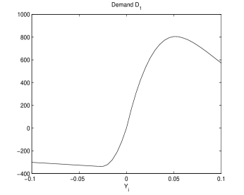
We assume that there is a second type of traders which are closely related to the prospect theory. The cumulative demand of this type of traders, $D_{2}$, is assumed to have a prospect pattern, as shown in Figure 3. Its derivative $D_{2}^{\prime}$ is also drawn.

(a) $D_{2}$

(b) $D_{2}^{\prime}$

Figure 3: Cumulative demand as a function of yield

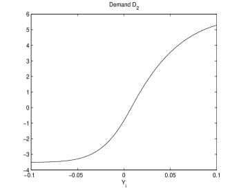
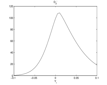
In our model, the function $D_{2}^{\prime}$ is given by

$$D_{2}^{\prime}(y)=\left\{\begin{aligned} &110e^{-150|x-0.008|^{1.5}},&\ x\leqslant 0.008,\\ &110e^{-40|x-0.008|^{1.3}},&\ x>0.008,\end{aligned}\right.$$

and $D_{2}(y)$ is the numerical integral of $D_{2}^{\prime}(y)$ with $D_{2}(0.008)=0$.

The change of demand in discrete time is given by $D_{2}(Y_{i+1})-D_{2}(Y_{i})$. If the first order approximation is used, we get $D_{2}(Y_{i+1})-D_{2}(Y_{i})\approx D_{2}^{\prime}(Y_{i})(Y_{i+1}-Y_{i})$. That is, their excessive demand of the asset is proportional to the change of $Y_{i}$, and the rate equals $D_{2}^{\prime}(Y_{i})$. When $\Delta Y_{i}>0$, their excessive demand increases, and when $\Delta Y_{i}<0$, their excessive demand decreases, and the rate equals $D_{2}^{\prime}(Y_{i})$. To be more specific, when $Y_{i}$ is already very high (or very low), their excessive demand is not very sensitive to $\Delta Y_{i}$. One explanation is that $Y_{i}$ is often thought to be a mean reverting process, and when $Y_{i}$ is very high (or very low), the probability that this return process stays high (or low) is small, and as a consequence, the excessive demand of this type of traders is insensitive to $\Delta Y_{i}$ in this case.

So far we have introduced the concept of prospect agents (traders), which is novel to our knowledge. In the next section, by assuming the existence of the usual noisy demand and trend chasing demand as in [17], we shall derive an ARCH model for $Y_{i}$.

2.2 An ARCH Model for the Yield Process

Let $\nu W_{t}$ be the cumulative noisy demand and $\xi\log P_{t}$ be the cumulative trend chasing demand as in [17], and $W_{t}$ is a Wiener process, $\nu<0$, $\xi>0$ are constants. The market clearing condition states that

$$\nu W_{t}+\xi\log P_{t}+\int_{0}^{t}D_{1}(Y_{t})dt+D_{2}(Y_{t})=M,$$

where $M$ is a constant. Define $\Delta W_{i}=W_{t_{i+1}}-W_{t_{i}}$, $\Delta t=t_{i+1}-t_{i}$, $i=0,1,...,n$, and $\Delta W_{i}$ is assumed to follow the normal $N(0,\Delta t)$ distribution. Since we are interested in the daily yield process, we choose $\Delta t=1/252$. The associated difference model can be easily written as follows

$$\nu\Delta W_{i}+\xi Y_{i+1}+D_{1}(Y_{i})\Delta t+D_{2}^{\prime}(Y_{i})(Y_{i+1}-Y_{i})=0,\ \ i=0,1,...,n,\ \ t=n\cdot\Delta t.$$ (2)

Now it is a simple step to derive a recursive equation for $Y_{i}$ by rewriting (2) as

$$\begin{split}Y_{i+1}&=\frac{D_{2}^{\prime}(Y_{i})Y_{i}-D_{1}(Y_{i})\Delta t}{\xi+D_{2}^{\prime}(Y_{i})}+\frac{-\nu}{\xi+D_{2}^{\prime}(Y_{i})}\Delta W_{i}\\ &=\frac{D_{2}^{\prime}(Y_{i})Y_{i}-D_{1}(Y_{i})\Delta t}{\xi+D_{2}^{\prime}(Y_{i})}+\frac{-\nu}{\sqrt{252}(\xi+D_{2}^{\prime}(Y_{i}))}\sqrt{252}\Delta W_{i}\\ &=f(Y_{i})+g(Y_{i})\epsilon_{i},\end{split}$$ (3)

where

$$f(Y_{i})=\frac{D_{2}^{\prime}(Y_{i})Y_{i}-D_{1}(Y_{i})\Delta t}{\xi+D_{2}^{\prime}(Y_{i})},\ \ \ \ \ \ g(Y_{i})=\frac{-\nu}{\sqrt{252}(\xi+D_{2}^{\prime}(Y_{i}))},$$

and $\epsilon_{i}=\sqrt{252}\Delta W_{i},\ i=1,2,...$ are i.i.d $N(0,1)$ random variables.

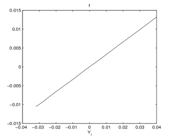
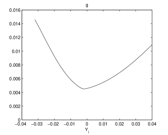
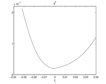
For the given functions $D_{1}$ and $D_{2}^{\prime}$ and the parameter settings $\xi=40,\nu=-27$, we can plot the graphs of $f(\cdot)$, $g(\cdot)$ and $g^{2}(\cdot)$ as shown in Figure 4.

(a) $f$

(b) $g$

(c) $g^{2}$

Figure 4: Drift and volatility functions

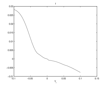
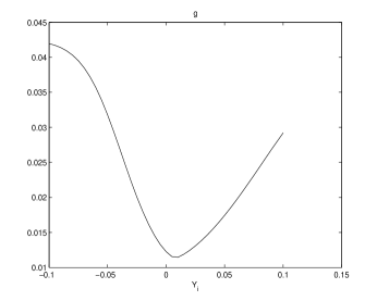
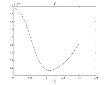
It can be easily seen from Figure 4 that there are patterns. For the function $f$, when $y>0$, $f(y)$ tends to be close to zero, and when $y$ is bigger, $f(y)$ is slightly negative. When $y<0$ is small, $f(y)$ tends to be positive, and if $y$ is way below zero, $f(y)$ tends to be bigger. In other words, if $Y_{i}$ is positive, on expectation, $Y_{i+1}$ will be negative, and if $Y_{i}$ is negative, on expectation, $Y_{i+1}$ will be positive. For the volatility $g^{2}$, its graph shows a ‘U-shaped’ smiling face.

3 Data Calibration

Local polynomial regression [27] [8] is used to estimate the drift (f) and volatility (g) functions. Let $\{Y_{t}\}$ be a time series, we want to fit an ARCH model so that

$$Y_{i}=f(Y_{i-1})+g(Y_{i-1})\epsilon_{i},$$

where $\epsilon_{i}$ are i.i.d. $N(0,1)$ random variables. The procedure is as follows: we seek a function $g(x)$ which satisfies

$$g^{2}(x)=E(Y_{i}^{2}|Y_{i-1}=x)-E^{2}(Y_{i}|Y_{i-1}=x).$$

Let $n$ be the size of $\{Y_{t}\}$, then for each $x$, consider the following two minimization problems:

$$\begin{split}&[\alpha_{1}(x),\alpha_{2}(x),\alpha_{3}(x)]\\ &=arg\min_{\alpha_{1},\alpha_{2},\alpha_{3}}\sum_{i=1}^{n}\left(Y_{i}^{2}-\alpha_{1}-\alpha_{2}\left(\frac{Y_{i-1}-x}{h}\right)-\frac{\alpha_{3}}{2}\left(\frac{Y_{i-1}-x}{h}\right)^{2}\right)K\left(\frac{Y_{i-1}-x}{h}\right),\end{split}$$ (4)

$$\begin{split}&[\beta_{1}(x),\beta_{2}(x),\beta_{3}(x)]\\ &=arg\min_{\beta_{1},\beta_{2},\beta_{3}}\sum_{i=1}^{n}\left(Y_{i}-\beta_{1}-\beta_{2}\left(\frac{Y_{i-1}-x}{h}\right)-\frac{\beta_{3}}{2}\left(\frac{Y_{i-1}-x}{h}\right)^{2}\right)^{2}K\left(\frac{Y_{i-1}-x}{h}\right),\end{split}$$ (5)

where $K(\cdot)$ denotes a nonnegative weight function and $h$ is a positive number called the bandwidth. We choose $K$ to be the standard normal pdf. Then $g^{2}(x)$ is estimated by $\hat{g}^{2}(x)=\alpha_{1}(x)-\beta_{1}^{2}(x)$, and the estimation of $f$ is given by $\hat{f}(x)=\beta_{1}(x)$.

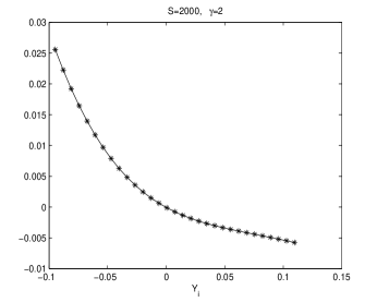
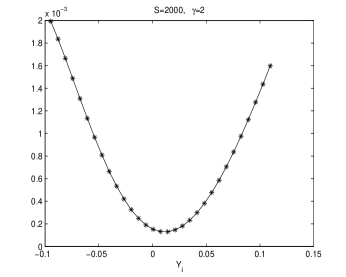
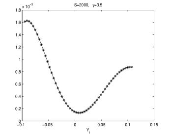
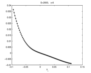
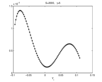
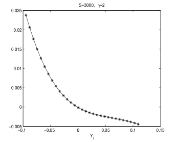
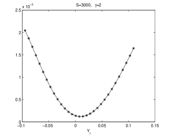
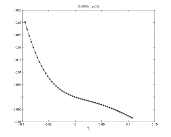
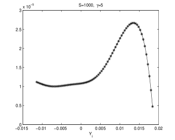
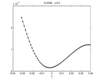
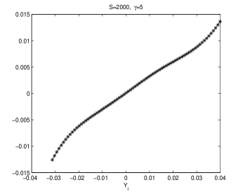
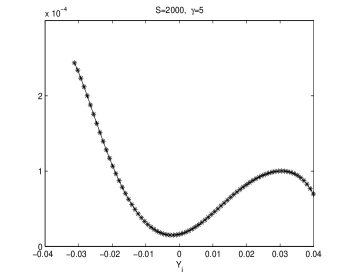
Let $\{P_{i}\}$ be the daily data of S&P500 index where the last date is 5/2/2013, and let $\{Y_{i}\}$ be the yield process, i.e., $Y_{i}=\log P_{i}-\log P_{i-1}$. For each data size $S$, we choose the bandwidth $h$ to be $h=\{\max(Y_{i})-\min(Y_{i})\}/{\gamma}$, where all $Y_{i}$’s belong to this set and $\gamma$ is a chosen positive constant. In what follows we shall pick different data sizes and different values of $\gamma$, and plot the graphs of $\hat{f}$ and $\hat{g}^{2}$.

(a) $\hat{f}$

(b) $\hat{g}^{2}$

Figure 5: $S=1000,\gamma=2$

(a) $\hat{f}$

(b) $\hat{g}^{2}$

Figure 6: $S=1000,\gamma=3.5$

(a) $\hat{f}$

(b) $\hat{g}^{2}$

Figure 7: $S=1000,\gamma=5$

(a) $\hat{f}$

(b) $\hat{g}^{2}$

Figure 8: $S=2000,\gamma=2$

(a) $\hat{f}$

(b) $\hat{g}^{2}$

Figure 9: $S=2000,\gamma=3.5$

(a) $\hat{f}$

(b) $\hat{g}^{2}$

Figure 10: $S=2000,\gamma=5$

(a) $\hat{f}$

(b) $\hat{g}^{2}$

Figure 11: $S=3000,\gamma=2$

(a) $\hat{f}$

(b) $\hat{g}^{2}$

Figure 12: $S=3000,\gamma=3.5$

(a) $\hat{f}$

(b) $\hat{g}^{2}$

Figure 13: $S=3000,\gamma=5$

From Figures 5 through 13, we can observe the following phenomena.

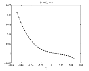
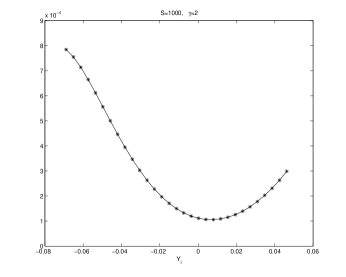
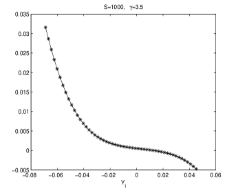
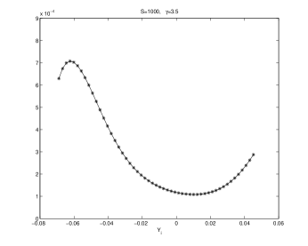
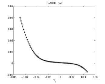
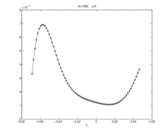
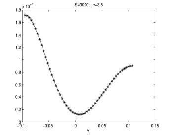
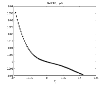
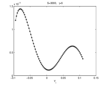
Observations:

1. There is a pattern of $\hat{f}$. If $Y_{i}=y>0$, $f(Y_{i})$ is slightly negative. If $Y_{i}<0$, $f(Y_{i})$ is positive. That means, if $Y_{i}>0$, i.e., there is a gain at time $t_{i}$, then on expectation, $Y_{i+1}$ tends to be slightly negative, i.e., there will be a slight loss at time $t_{i+1}$. However, if $Y_{i}<0$, i.e., there is a loss at time $t_{i}$, then on expectation, $Y_{i+1}$ tends to be big, i.e., there will be a big gain at time $t_{i+1}$. This represents a mean reverting pattern.

2. All the graphs of $\hat{g}^{2}$ show U-shaped ‘smiling faces’, and the minimum is achieved at a point of $Y_{i}$ close to zero. In fact, a point that is slightly to the right of zero. What is more, on each ‘smiling face’, the left side of the curve is higher than the right side of the curve. So these are tilted ‘smiling faces’, or skew.

3. When the data size is small, e.g., $S=1000$, we observe the boundary effect on the edges of the interval, see, e.g., the graphs of $\hat{g}^{2}$. This phenomenon was also observed in [27] where an explanation was also provided.

If we compare Figures 5 through 13 with Figure 4, we can see that model (3) provides a good fit.

4 The Implied Volatility

Since $Y_{i}=\log P_{i}-\log P_{i-1}$, we can rewrite model (3) as

$$\log P_{i+1}-\log P_{i}=f(\log P_{i}-\log P_{i-1})+g(\log P_{i}-\log P_{i-1})\epsilon_{i},i=1,2,...$$

which provides us an ARCH model for the process $\log P_{i}$ as follows

$$\log P_{i+1}=\log P_{i}+f(\log P_{i}-\log P_{i-1})+g(\log P_{i}-\log P_{i-1})\epsilon_{i},i=1,2,...$$ (6)

We shall use this model as the fundamental to study the option pricing problem. In doing this, it might be easier to use a simple polynomial regression to approximate $f$ and $g$, and we get the following ARCH model

$$\begin{split}\log P_{i+1}=&\log P_{i}\\ &-8.948\times 10^{-5}-7.557\times 10^{-2}Y_{i}+0.8305Y_{i}^{2}-13.60Y_{i}^{3}+52.84Y_{i}^{4}\\ &+\left(1.288\times 10^{-2}-0.1138Y_{i}+5.503Y_{i}^{2}+6.492Y_{i}^{3}-3.306\times 10^{2}Y_{i}^{4}\right)\epsilon_{i},\end{split}$$ (7)

where $Y_{i}=\log P_{i}-\log P_{i-1}$. That is,

$$\begin{split}\tilde{f}(Y_{i})&=-8.948\times 10^{-5}-7.557\times 10^{-2}Y_{i}+0.8305Y_{i}^{2}-13.60Y_{i}^{3}+52.84Y_{i}^{4},\\ \tilde{g}(Y_{i})&=1.288\times 10^{-2}-0.1138Y_{i}+5.503Y_{i}^{2}+6.492Y_{i}^{3}-3.306\times 10^{2}Y_{i}^{4},\end{split}$$

where $\tilde{f},\tilde{g}$ represent the polynomial approximations of $f,g$, respectively. Figure (14) shows the graphs of $\tilde{f},\tilde{g}$ and $\tilde{g}^{2}$.

(a) $\tilde{f}$

(b) $\tilde{g}$

(c) $\tilde{g}^{2}$

Figure 14: Polynomial Approximations of $f,g,g^{2}$

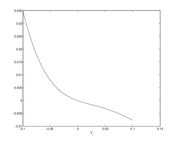
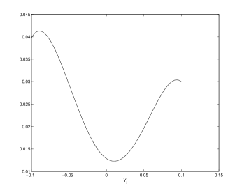
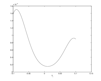
It can be seen that this model is a local volatility model, but different from most well known local volatility models which aimed to replicate the implied volatility surface only, our model replicates both the drift term and volatility term, through real data calibration using the technique of local polynomial regression.

Now the model (10) is easy to use in a Monte Carlo simulation. In order to get the fair price of the European call options, we rewrite this model under the risk neutral measure and get

$$\log P_{i+1}-\log P_{i}=(r-\frac{1}{2}\sigma^{2}(Y_{i}))\Delta t+\sigma(Y_{i})\sqrt{\Delta t}\tilde{\epsilon}_{i},$$ (8)

where $r$ is the risk free interest rate, $Y_{i}=\log P_{i}-\log P_{i-1}$, $\tilde{\epsilon}_{i}$ is the standard normal random variable under the risk neutral measure, and

$$\sigma(Y_{i})=\tilde{g}(Y_{i})/\sqrt{\Delta t}.$$

In order to find a proper number of paths, we use Monte Carlo simulation to price a European call option with the following parameter settings: annual interest rate $r=0.03$, time to maturity $T=60$ months, strike price $K=800$ and underlying price $P_{0}=1462.42,P_{1}=1459.37$. We chose this option because it has the largest variance in our model. The number of paths ranges from 10,000 to 1,000,000, and for each setting, 20 trials are run and the standard deviation of the option prices are calculated. The result is shown in Figure 15.

Figure 15: Standard Deviation

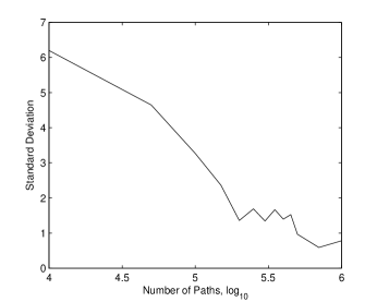
We can now set the number of paths to be 200,000. Figure 16 shows a Monte Carlo simulation on call option prices with 200,000 sample paths.

Figure 16: Call Options Prices

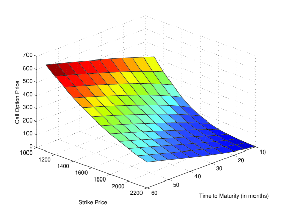
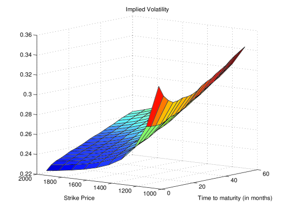
We pick the region $1100\leq K\leq 2000$ and $6\leq T\leq 60$ to recover the implied volatility surface from the Black-Scholes formula. The reason is that, on this region the computation is considered to be stable because $Vega$ is not too close to zero. A detailed explanation on this issue is provided in the Appendix. Figure 17 shows the implied volatility surface through the Black-Scholes formula.

Figure 17: Implied Volatility Surface

5 Foreign Currency Market

In this section, we shall construct an ARCH model for risky assets on currency market. Let $P_{i}$ be the USD/GBP exchange rate, and we again use the same model:

$$Y_{i+1}=f(Y_{i})+g(Y_{i})\epsilon_{i},$$ (9)

where

$$f(Y_{i})=\frac{D_{2}^{\prime}(Y_{i})Y_{i}-D_{1}(Y_{i})\Delta t}{\xi+D_{2}^{\prime}(Y_{i})},\ \ \ \ \ \ g(Y_{i})=\frac{-\nu}{\sqrt{252}(\xi+D_{2}^{\prime}(Y_{i}))},$$

$Y_{i}=\log P_{i}-\log P_{i-1}$, and $\epsilon_{i}=\sqrt{252}\Delta W_{i},\ i=1,2,...$ are i.i.d $N(0,1)$ random variables.

There are obviously some differences in the currency market. Realistically, unlike the stock market, one can not expect that $P_{i}$ (USD/GBP) increases exponentially at a certain speed. It is commonly believed that $P_{i}$ shows a mean reverting dynamics. Therefore, if there is a big jump of $P_{i}$ in one day, due to the prospect theory, more holders tend to sell the share in order to realize the profit, showing an extreme risk averse behavior, and vice versa. Therefore, the demand $D_{1}$ in the currency market is believed to show a stronger prospect phenomenon than that on the stock market. Here the function $D_{1}(y)$ is assumed to take the following form:

$$D_{1}(y)=\left\{\begin{aligned} &5.381+4.039\times 10^{4}y+2.169\times 10^{6}y^{2}+2.802\times 10^{7}y^{3},&\ y\leqslant 0\\ &-3.27+3.391\times 10^{4}y-1.056\times 10^{6}y^{2}+7.935\times 10^{6}y^{3},&\ y>0\end{aligned}\right.$$

and its graph is shown in Figure 18.

Figure 18: Excessive demand as a function of yield

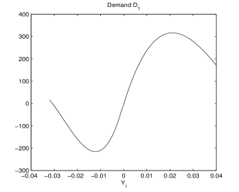
It can be seen that if $Y_{i}$ is much bigger than zero, $D_{1}$ decreases, showing an extreme risk averse behavior; and if $Y_{i}$ is far below zero, $D_{1}$ increases, showing an extreme risk seeking behavior.

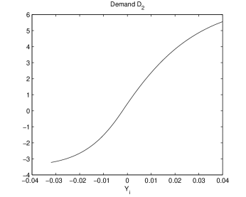
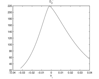
The function $D_{2}^{\prime}$ in this model is given by

$$D_{2}^{\prime}(y)=\left\{\begin{aligned} &220e^{-250|x+0.002|^{1.36}},&\ x\leqslant-0.002,\\ &220e^{-100|x+0.002|^{1.35}},&\ x>-0.002,\end{aligned}\right.$$

and $D_{2}(y)$ is the numerical integral of $D_{2}^{\prime}(y)$ with $D_{2}(-0.002)=0$. The center point $-0.002$ is very close to and even slightly less than zero, showing that $P_{i}$ is not expected to increase exponentially at a certain speed, but rather, $Y_{i}=\log P_{i}-\log P_{i-1}$ is expected to stay around zero. The graphs of $D_{2},D_{2}^{\prime}$ are shown in Figure 19.

(a) $D_{2}$

(b) $D_{2}^{\prime}$

Figure 19: Cumulative demand as a function of yield

With the parameter settings $\xi=60$, $\nu=-20$, we plot the functions $f,g,g^{2}$ in Figure 20.

(a) $f$

(b) $g$

(c) $g^{2}$

Figure 20: Drift and volatility functions

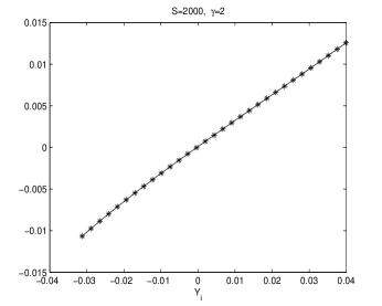
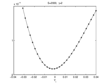
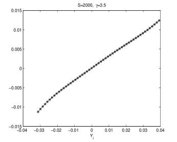
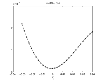
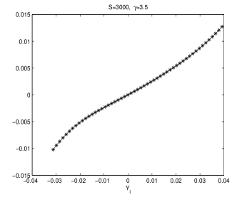
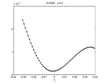
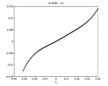
Once again the graphs of $g,g^{2}$ show ‘smiling faces’, which are comparatively more symmetric than that in Figure 4. However, the graph of $f$ shows a very different pattern. It can be seen that $f(Y_{i})$ is an increasing function in $Y_{i}$, which means, if $Y_{i}$ is positive, then on expectation, $Y_{i+1}$ tends to be positive, and this tendency is expected to last for several days. On the contrary, if $Y_{i}$ is negative, $Y_{i+1}$ tends to be negative and this pattern may last for some time, expectedly. Also we notice that the slope of $f(Y_{i})$ is less than $1$, which indicates that $Y_{i+1}=f(Y_{i})$($i\to\infty$) converges to zero if only the drift term is considered.

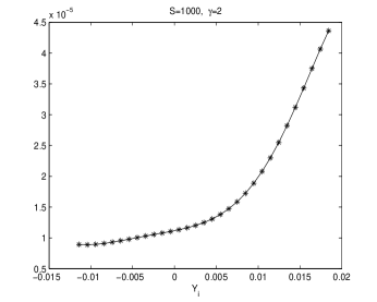
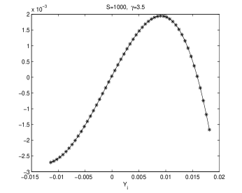
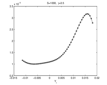
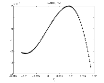
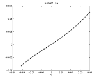
We use real market data and local polynomial regression to estimate the functions $f$ and $g^{2}$. Let $P_{i}$ be the USD/GBP exchange rate, where the last date in the data set is 5/21/2013. Different data sizes and bandwidths are chosen and the result is shown in Figures 21-29.

(a) $\hat{f}$

(b) $\hat{g}^{2}$

Figure 21: $S=1000,\gamma=2$

(a) $\hat{f}$

(b) $\hat{g}^{2}$

Figure 22: $S=1000,\gamma=3.5$

(a) $\hat{f}$

(b) $\hat{g}^{2}$

Figure 23: $S=1000,\gamma=5$

(a) $\hat{f}$

(b) $\hat{g}^{2}$

Figure 24: $S=2000,\gamma=2$

(a) $\hat{f}$

(b) $\hat{g}^{2}$

Figure 25: $S=2000,\gamma=3.5$

(a) $\hat{f}$

(b) $\hat{g}^{2}$

Figure 26: $S=2000,\gamma=5$

(a) $\hat{f}$

(b) $\hat{g}^{2}$

Figure 27: $S=3000,\gamma=2$

(a) $\hat{f}$

(b) $\hat{g}^{2}$

Figure 28: $S=3000,\gamma=3.5$

(a) $\hat{f}$

(b) $\hat{g}^{2}$

Figure 29: $S=3000,\gamma=5$

Observations:

1. When the data size is small, e.g., $S=1000$, the boundary effect is very significant. Similar graphs are found in [27].

2. When $S=2000$ or $S=3000$, $\hat{f}(Y_{i})$ is increasing and almost linear in $Y_{i}$, but the slope of the graph is less than $1$.

3. Graphs of $\hat{g}^{2}$ all show ‘smiling faces’.

In order to construct an ARCH model for $P_{i}$, we use polynomial approximations of the functions $f$ and $g$. Let $\tilde{f}$, $\tilde{g}$ be the polynomial approximations of the functions $f,g$ respectively, where $\tilde{f}(Y_{i})=0.33Y_{i}$,

$$\begin{split}\tilde{g}(Y_{i})=&4.328\times 10^{-3}+6.422\times 10^{-2}Y_{i}+15.73Y_{i}^{2}\\ &-2.934\times 10^{2}Y_{i}^{3}-6.987\times 10^{3}Y_{i}^{4}+1.542\times 10^{5}Y_{i}^{5},\end{split}$$

then we may plot the graphs of $\tilde{g},\tilde{g}^{2}$ in Figure 30.

(a) $\tilde{g}$

(b) $\tilde{g}^{2}$

Figure 30: Polynomial approximations of $g,g^{2}$

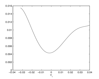
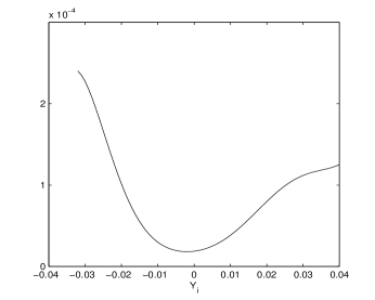
With this setting the following ARCH model is obtained:

$$\begin{split}\log P_{i+1}=&\log P_{i}+0.33Y_{i}\\ &+(4.328\times 10^{-3}+6.422\times 10^{-2}Y_{i}+15.73Y_{i}^{2}\\ &-2.934\times 10^{2}Y_{i}^{3}-6.987\times 10^{3}Y_{i}^{4}+1.542\times 10^{5}Y_{i}^{5})\epsilon_{i},\end{split}$$ (10)

where $Y_{i}=\log P_{i}-\log P_{i-1}$.

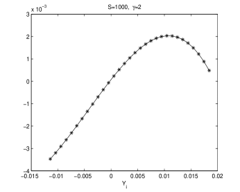
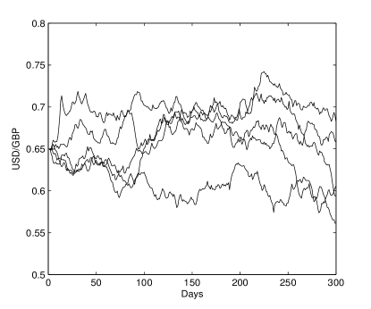
To illustrate the properties we observed, we randomly generate some sample paths of $P_{i}$ according to the model (10) with starting points $P_{1}=0.6493$, $P_{2}=0.6492$, and the result is shown in Figure 31.

Figure 31: Sample paths

6 Conclusions

In this paper we introduced the prospect agents as the market participants. Based on the fact that asset price is generated by the temporary balance between supply and demand, we model the price fluctuation through the microeconomic approach. The prospect agents’ reactions to gains and losses affect the price process through the feedback effect. If they experience gains of their investment based on their expectation, the prospect agents illustrate a risk averse behavior on their demand, while if they experience losses, they often show a risk seeking behavior. Then ARCH models are constructed for both the S&P500 index process and the USD/GBP exchange rate, respectively. Through this model we could reproduce the volatility smile phenomenon on options that is well observed in actual financial market. To the best of our knowledge, we are the first to explain the volatility smile/skew through prospect theory.

This paper provides a new approach and a framework to construct discrete and possibly continuous models for asset prices. Future research may focus on parameter estimation and extending this method to model the price fluctuations of other financial products.

Appendix

In this section we shall discuss a numerical issue on recovering the implied volatility surface from Black-Scholes formula. It is well known that the implied volatility of actual option prices does not equal a constant, but shows a volatility skew for equity options or volatility smile for foreign exchange contracts. Many models have been developed to replicate this phenomenon. For example, the local volatility model [6], the stochastic volatility model [15], and the Jump-Diffusion models [5][20].

When a model is presented, very often one uses Monte Carlo simulation to find the options prices and put them in Black-Scholes formula to find the implied volatilities. Then an implied volatility surface can be found, and if it mimics the actual volatility surface, one claims that this model is a good one. However, there is a numerical issue involved. Even if the classical geometric Brownian motion model $dP_{t}=rP_{t}dt+\sigma P_{t}dW_{t}$ with constant volatility is used in the Monte Carlo simulation, it is very hard to recover $\sigma$ as a constant if the aforementioned procedure is implemented. Of course the price generated by Monte Carlo simulation can not perfectly replicate the Black-Scholes price due to the computer generated pseudo random numbers. But even if the error between these two prices is tiny, in some cases the implied volatility is quite different from $\sigma$. The reason behind this is due to $Vega$, and in some situations the option price is extremely insensitive to volatility. That means, on the contrary, even if there is a tiny error on the option price, there will be a big error between the implied volatility and $\sigma$. In what follows we shall study the cases where $Vega$ is small, i.e., option price is insensitive to volatility.

We first write out the Black-Scholes formula for European call option,

$$\begin{split}C&=P\Phi(d_{1})-e^{-rT}K\Phi(d_{2}),\\ d_{1}&=\frac{\ln(P/K)+(r+0.5\sigma^{2})T}{\sigma\sqrt{T}},\\ d_{2}&=d_{1}-\sigma\sqrt{T},\end{split}$$

where $r$ is the annual interest rate, $P$ is the spot price, $K$ is the strike price, $T$ is the time to maturity, and $\Phi$ is the standard normal distribution function. The $Vega$ is given by

$$\frac{\partial C}{\partial\sigma}=P\phi(d1)\sqrt{T},$$ (11)

where $\phi$ is the standard normal probability density function. We pick the values $P=1459.37$, $r=0.03$, $\sigma=0.15$, and plot the $Vega$ as a function of both $T$ and $K$ in Figure 32.

Figure 32: $Vega$, $\sigma=0.15$

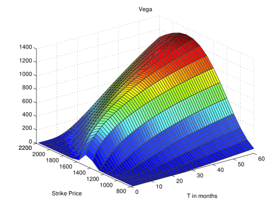
The strike price ranges from $800$ to $2200$ and $T$ ranges from $1$ to $60$ months. It can be easily seen that when $K$ is much lower or much higher than the spot price, and $T$ is small, the $Vega$ is very small. For example, $Vega(K,T)=Vega(800,1)=7.824541295983192\times 10^{-041}$. That means, even if there is a tiny error in the pricing of options, the implied volatility could be very different from the true $\sigma$. We then change the value of $\sigma$ to $0.3$ and plot the $Vega$ in Figure 33, and we see a similar pattern.

Figure 33: $Vega$, $\sigma=0.3$

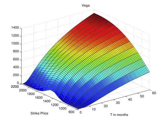
In a typical research on implied volatility surface, unfortunately, the region where the volatility skew/smile is observed coincides with the region where $Vega$ is small. That means, even if an implied volatility surface is obtained which is similar to the actual volatility surface of market data, the result is skeptical if the effect of $Vega$ was not considered.

As a conclusion, in order to find the correct implied volatility through the Black-Scholes formula, the computation should be executed over the region where $Vega$ is not close to zero. Typically this is the region where $T$ is not too small, $K$ is close to the curve of $Pe^{rT}$, and the true volatility is not too small, see Figures 32 and 33.

References

- [1] E. Barucci, P. Malliavin, M.E. Mancino, R. Renò and A. Thalmaier, The Price-Volatility Feedback Rate: An Implementable Mathematical Indicator of Market Stability, Mathematical Finance, 13(1) (2003) 17–35.
- [2] E. Bayraktar, U. Horst and R. Sircar, Queueing Theoretic Approaches to Financial Price Fluctuations, Handbooks in Operations Research and Management Science, 15 (2007) 637–677.
- [3] N. P.B. Bollen, Valuing Options in Regime-Switching Models, The Journal of Derivatives, 6(1) (1998) 38–49.
- [4] A. Danilova, Emergence of Stochastic Volatility from Informational Heterogeneity, Doctoral Dissertation, Princeton University (2005).
- [5] D. Duffie, J. Pan and K. Singleton, The Transform Analysis and Asset Pricing for Affine Jump-Diffusions, Econometrica, 68 (6) (2000) 1343–1376.
- [6] B. Dupire, Pricing with a Smile, Risk, (1994) 18–20.
- [7] R. Engle, Autoregressive Conditional Heteroskedasticity with Estimates of the Variance of U.K. Inflation, Econometrica, 50 (1982) 987–1008.
- [8] E. Masry and J. Fan, Local Polynomial Estimation of Regression functions for mixing processes, Scandinavian Journal of Statistics, 24 (1997) 165–179.
- [9] H. Föllmer and M Schweizer, A Microeconomic Approach to Diffusion Models for Stock Prices, Mathematical Finance 3 (1993) 1–23.
- [10] H. Föllmer, U. Horst and A. Kirman, Equilibria in Financial Markets with Heterogeneous Agents: A Probabilistic Perspective, Journal of Mathematical Economics, 41 (2005) 123–155.
- [11] J.P. Fouque, G. Papanicolaou and R. Sircar, Mean-Reverting Stochastic Volatility, International Journal of Theoretical and Applied Finance, 3(1) (2000) 101–142.
- [12] R. Frey and A. Stremme, Market Volatility and Feedback Effects from Dynamic Hedging, Mathematical Finance, 7(4) (1997) 351–374.
- [13] I. Goldstein and A. Guembel, Manipulation and the Allocational Role of Prices, Review of Economic Studies, 75 (2008) 133–164.
- [14] P. Heemeijer, C. Homoes, J. Sonnemans and J. Tuinstra, Price Stability and Volatility in Markets with Positive and Negative Expectations Feedback: An Experimental Investigation, Journal of Economic Dynamics and Control, 33 (2009) 1052–1072.
- [15] S. Heston, A Closed-Form Solution for Options with Stochastic Volatility with Applications to Bond and Currency Options, The Review of Financial Studies, 6(2) (1993) 327–343.
- [16] D. Hirshleifer, A. Subrahmanyam and S. Titman, Feedback and the success of irrational investors, Journal of Financial Economics, 81 (2006) 311–338.
- [17] U. Horst, Financial Price Fluctuations in A Stock Market Model with Many Interacting Agents, Economic Theory, 25 (2005) 917–932.
- [18] D. Kahneman and A. Tversky, Prospect Theory: An Analysis of Decision under Risk, Econometrica, 47(2) (1979) 263–292.
- [19] N. Khanna and R. Sonti, Value Creating Stock Manipulation: Feedback Effect of Stock Prices on Firm Value, Journal of Financial Markets, 7 (2004) 237–270.
- [20] S.G. Kou, A Jump-Diffusion Model for Option Pricing, Management Science, 48 (8), (2002) 1086–1101.
- [21] E. Ozdenoren and K. Yuan, Feedback Effects and Asset Prices, The Journal of Finance, LXIII(4) (2008) 1939–1975.
- [22] A. Papanicolaou and R. Sircar, A Regime-Switching Heston Model for VIX and S&P 500 Implied Volatilities, to appear in Quantitative Finance, 2013.
- [23] E. Platen and M. Schweizer, On Feedback Effects from Hedging Derivatives, Mathematical Finance, 8(1) (1998) 67–84.
- [24] H. Shefrin and M. Statman, The Disposition to Sell Winners Too Early and Ride Losers Too Long: Theory and Evidence, Journal of Finance, 40 (1985) 777–790.
- [25] A. Subrahmanyam and S. Titman, Feedback From Stock Prices to Cash Flows, Journal of Finance, 56 (2001) 2389–2413.
- [26] S. Taylor, Modeling Stochastic Volatility: A Review and Comparative Study, Mathematical Finance, 4 (1994) 183–204.
- [27] W. Härdle and A.B. Tsybakov, Local Polynomial Estimators of the Volatility Function in Nonparametric Autoregression, Journal of Econometrics, 81 (1997) 223–242.
- [28] D.D., Yao, Q. Zhang and X.Y. Zhou, A Regime-Switching Model for European Options, In Stochastic Processes, Optimization, and Control Theory Applications in Financial Engineering, Queueing Networks, and Manufacturing Systems, H. Yan, G. Yin and Q. Zhang (eds.), Springer, (2006) 281–300.