Average expansion rate and light propagation in a cosmological Tardis spacetime

Abstract

We construct the first exact statistically homogeneous and isotropic cosmological solution in which inhomogeneity has a significant effect on the expansion rate. The universe is modelled as a Swiss Cheese, with dust FRW background and inhomogeneous holes. We show that if the holes are described by the quasispherical Szekeres solution, their average expansion rate is close to the background under certain rather general conditions. We specialise to spherically symmetric holes and violate one of these conditions. As a result, the average expansion rate at late times grows relative to the background, i.e. backreaction is significant. The holes fit smoothly into the background, but are larger on the inside than a corresponding background domain: we call them Tardis regions. We study light propagation, find the effective equations of state and consider the relation of the spatially averaged expansion rate to the redshift and the angular diameter distance.

1 Introduction

The backreaction conjecture.

Predictions of homogeneous and isotropic models of the universe with ordinary matter (with non-negative pressure) and ordinary gravity (based on the four-dimensional Einstein-Hilbert action) disagree with observations of cosmological distances and average expansion rate at late times by a factor of two (see [2] for discussion and references). The problem is usually addressed by introducing exotic matter with negative pressure or modifying gravity on large scales, leading to accelerated expansion. However, it is possible that the failure of the predictions of homogeneous and isotropic models is related to the known breakdown of homogeneity and isotropy due to structure formation, rather than unknown fundamental physics.

An inhomogeneous and/or anisotropic space in general expands on average differently than a space that is exactly homogeneous and isotropic. This feature of general relativity is known as backreaction [3, 5, 4, 6, 7]; see [8, 9, 10, 11, 2] for reviews. The possibility that the change of the expansion rate due to structure formation would explain the observations of longer distances and faster expansion is called the backreaction conjecture [12, 13, 14, 15, 16]. Because of backreaction, the average expansion rate can accelerate even in a dust universe in which the local expansion rate decelerates everywhere [17, 18, 19, 20, 21]. Inhomogeneity also changes the relation between the expansion rate and distance, even in a statistically homogeneous and isotropic universe [22, 23, 24, 21], so explaining the observations does not necessarily require accelerating expansion. In Newtonian cosmology [5] and in relativistic perturbation theory [25] backreaction is small (the issue has also been studied with a non-standard perturbative formalism [26, 27]). Based on a gradient expansion, it has been argued that backreaction is expected to be small even in the non-linear regime of structure formation [28]. However, as the density contrast goes non-linear, gradients become large and the expansion breaks down. In a semirealistic statistical model, the magnitude of the observed change in the expansion rate and the timescale of ten billion years emerge from the physics of structure formation [29, 30]. There is no fully realistic calculation, and the amplitude of backreaction in the real universe remains an open question.

Expansion rate and light propagation.

In studies of backreaction, the average expansion rate and other spatial averages have often been considered without relating them to observables such as the redshift and the angular diameter distance. On the other hand, in most work on light propagation in inhomogeneous spacetimes it has been assumed, explicitly or implicitly, that the average expansion rate is the same as in the exactly homogeneous and isotropic Friedmann-Robertson-Walker (FRW) model [29].

In [18, 29] it was suggested that in statistically homogeneous and isotropic universes in which the distribution evolves slowly, light propagation over long distances could be described by a few average geometrical quantities, namely the scale factor (or equivalently the average expansion rate) and the average spatial curvature. In [22, 23] it was argued that redshift and angular diameter distance can, in a dust spacetime, be approximately calculated from just the average expansion rate and the value of the matter density today (the average spatial curvature at all times is not needed), and that null shear and light deflection are expected to remain small. Quantitative studies of light propagation were consistent with this idea in the weak sense that in statistically homogeneous and isotropic models in which the average expansion rate is close to the FRW case, deviations in the redshift and distance had been found to be small [29], and this is the case also for later studies [31, 32, 33, 34, 35, 37, 36]. The small anisotropy of the cosmic microwave background is also consistent with large deviation of the expansion rate from the FRW case [38].

Recently, the average expansion rate and light propagation have been considered in models that display either full or partial statistical homogeneity and isotropy. In the absence of such symmetry, there is no reason to expect the redshift and the distance to be calculable from the average expansion rate. Indeed, that is not the case in spherically symmetric models [39, 40, 41, 24].

Exact planar solutions with non-perturbative inhomogeneities have been studied in [42, 43]. In [42], the average expansion rate was not calculated, but for the geometry considered, it reduces to the FRW case when over- and underdensities are compensated along the line of sight, and in this case the redshift and the distance are also close to the FRW values. In [43], variations in the expansion rate similarly cancel, and results for light propagation are close to the FRW case. In [24], the relation between light propagation and the average expansion rate was studied in several settings, including a planar configuration with FRW and Kasner regions, as well as a model with alternating expanding and collapsing dust FRW regions. In contrast to previous studies, the average expansion rate in the models is different from the FRW case. The average expansion rate was found to give a good description of light propagation when the distribution along the light ray is statistically homogeneous. However, the model with alternating FRW regions (unlike the FRW-Kasner model) is not a solution of the Einstein equation, as the boundaries of different regions do not match together. In that model, there is also some arbitrariness in the way the time spent by the light ray in different regions was assigned.

The expansion rate and light propagation have also been studied in models with discrete matter distribution [45, 46]. The solutions of [45] are approximate and the results depend on the method used to join lattice cells together, with the more reliable method leading to only a small correction to the FRW results. In the perturbative calculation of [46], corrections to the FRW case were found to be small. This is in agreement with the general result that in the perturbative regime the average expansion rate and the redshift are close to the FRW case. This is likely also true for the distance if the universe is statistically homogeneous and isotropic [25]. Calculations for the distance in first and second order in perturbation theory agree with this conjecture [49, 50, 51].

These studies support the idea that the redshift and the angular diameter distance are determined by the average expansion rate when structures along the path of the light ray are a representative sample of those in the volume over which the average is taken. However, almost all exact solutions with statistical homogeneity (at least along the light ray) have had average expansion rate close to the FRW case, whereas models with average expansion rate very different from FRW have not been exact solutions. One exception is the Kasner-Eds model in [24], though it is not statistically isotropic.

We present the first statistically homogeneous and isotropic exact solution in which inhomogeneity has a significant impact on the expansion rate, and study the relation between the average expansion rate and light propagation. Our model is based on the Swiss Cheese construction [31, 20, 32, 34, 52, 35]. We start with a FRW dust model and replace some spherical regions with the most general known exact dust solution, the Szekeres model [53], [54] (page 387). In section 2 we prove that under certain general assumptions the average expansion rate of the Szekeres Swiss Cheese model is close to the background. In section 3 we present our cosmological model that violates one of these assumptions, specialising to the spherically symmetric subcase of the Szekeres model, the Lemaître-Tolman-Bondi (LTB) model [54] (page 294), [55, 56, 57]. The model has surface layers, which have a large effect on light propagation, and we consider modified versions of the redshift and the angular diameter distance that are less affected by the surface layers. We study how well the redshift and the distance are described by the average expansion rate, and consider effective equations of state. In section 4 we discuss the results and their relation to previous work. In section 5 we summarise our findings and mention possible directions for extending the work.

2 Szekeres Swiss Cheese

2.1 The Szekeres model

The metric, equations of motion and solutions.

We consider inhomogeneous dust solutions (“holes”) embedded in a FRW dust model (“background” or “cheese”). We take the cosmological constant to be zero, so the Einstein equation is

$$G_{\alpha\beta}=8\pi G_{\mathrm{N}}T_{\alpha\beta}=8\pi G_{\mathrm{N}}\rho_{\mathrm{m}}u_{\alpha}u_{\beta}\ ,$$ (2.1)

where $G_{\mathrm{N}}$ is Newton’s constant, $\rho_{\mathrm{m}}$ is the dust energy density (we assume $\rho_{\mathrm{m}}\geq 0$) and $u^{\alpha}=\delta^{\alpha}_{\ \,0}$ is the four-velocity of observers comoving with the dust. The solution can have surface layers, their contribution is not included in (2.1).

The most general known exact solution of (2.1) is the Szekeres model [53], [54] (page 387). The solution does not have any symmetries, i.e. there are no Killing vectors, but the form of the metric is nevertheless rather constrained. In comoving synchronous coordinates the metric can be written as

$$\mathrm{d}s^{2}=-\mathrm{d}t^{2}+X(t,r,p,q)^{2}\mathrm{d}r^{2}+\frac{R(t,r)^{2}}{\mathscr{E}(r,p,q)^{2}}(\mathrm{d}p^{2}+\mathrm{d}q^{2})\ ,$$ (2.2)

where $t$ is the proper time of observers comoving with the dust fluid. Hypersurfaces of constant $t$ and $r$ are called shells. The functions $X$ and $\mathscr{E}$ are (we choose $X\geq 0$)

$$X(t,r,p,q) = \frac{|R^{\prime}-R\frac{\mathscr{E}^{\prime}}{\mathscr{E}}|}{\sqrt{\epsilon+E(r)}}$$ (2.3)

$$\mathscr{E}(r,p,q) = \frac{S(r)}{2}\left[\left(\frac{p-P(r)}{S(r)}\right)^{2}+\left(\frac{q-Q(r)}{S(r)}\right)^{2}+\epsilon\right]\ ,$$ (2.4)

where $E(r)\geq-1,S(r),P(r)$ and $Q(r)$ are free functions, prime denotes derivative with respect to $r$ and the parameter $\epsilon$ takes on values $+1,0,-1$, respectively called the quasispherical, quasiplanar and quasihyperbolic solutions. When $\epsilon\geq 0$, the coordinates $p$ and $q$ take values in the range $]-\infty,\infty[$; see [53] for the case $\epsilon=-1$. The range of the $t$- and $r$-coordinates depends on the specific solution. In the cases with $\epsilon\leq 0$, the volume of the shells is infinite, so because we are interested in holes with finite volume, only the quasispherical solution with $\epsilon=+1$ is relevant. (We do not consider non-trivial topologies, which could make the hypersurfaces compact.) The function $R(t,r)\geq 0$ satisfies the equations

$$\dot{R}(t,r)^{2} = \frac{2M(r)}{R(t,r)}+E(r)$$ (2.5)

$$\rho_{\mathrm{m}}(t,r,p,q) = \frac{1}{4\pi G_{\mathrm{N}}}\frac{M^{\prime}-3M\frac{\mathscr{E}^{\prime}}{\mathscr{E}}}{R^{2}\left(R^{\prime}-R\frac{\mathscr{E}^{\prime}}{\mathscr{E}}\right)}\ ,$$ (2.6)

where dot denotes derivative with respect to $t$ and $M(r)$ is a free function with the dimension of length. The solutions of (2.5) are as follows.

For $E(r)<0$,

$$R(t,r)=\frac{M}{|E|}(1-\cos\eta)\ ,\quad\eta-\sin\eta=\frac{|E|^{3/2}}{M}(t-{t_{\mathrm{B}}}(r))\ .$$ (2.7)

For $E(r)=0$,

$$R(t,r)=\left(\frac{9}{2}M(t-{t_{\mathrm{B}}}(r))^{2}\right)^{1/3}\ .$$ (2.8)

For $E(r)>0$,

$$R(t,r)=\frac{M}{E}(\cosh\eta-1)\ ,\quad\sinh\eta-\eta=\frac{E^{3/2}}{M}(t-{t_{\mathrm{B}}}(r))\ .$$ (2.9)

Here ${t_{\mathrm{B}}}(r)$ is a free function that indicates the time when the big bang happens at radius $r$. Time-reversed versions of (2.7)–(2.9), where ${t_{\mathrm{B}}}(r)$ indicates the big crunch time instead, are also solutions. In addition to the big bang or big crunch, Szekeres models can also have shell crossing singularities [53, 58, 59]. We consider only models that are free of shell crossings at least up to the present day.

Subcases.

When $\mathscr{E}^{\prime}=0$, we have the isotropic subcase of the Szekeres model, the LTB model [54] (page 294), [55, 56, 57]. In this case, $R$ is the areal radius and $R_{\mathrm{p}}\equiv\int_{0}^{r}\mathrm{d}r^{\prime}X(t,r^{\prime})\geq 0$ is the proper radius of a sphere centred on $r=0$. The function $X$ reduces to

$$X(t,r)=\frac{|R^{\prime}(t,r)|}{\sqrt{1+E(r)}}\equiv\frac{R^{\prime}(t,r)}{\sqrt{1+E(r)}}s(r)\ ,$$ (2.10)

where $s(r)\equiv\mathrm{sign}(R^{\prime})$ (any zeroes of $R^{\prime}$ have to be at constant $r$ for the density (2.6) to be non-divergent). For observers comoving with the dust fluid, the volume expansion rate $\theta$, shear tensor $\sigma^{\alpha}_{\ \beta}$, and spatial curvature ${{}^{(3)}R}$ are (for the definitions, see [60, 61, 62, 63, 64])

$$\theta = 2\frac{\dot{R}}{R}+\frac{\dot{R}^{\prime}}{R^{\prime}}$$

$$\sigma^{\alpha}_{\ \beta} = \mathrm{diag}\left(0,\frac{2}{3},-\frac{1}{3},-\frac{1}{3}\right)\left(\frac{\dot{R}^{\prime}}{R^{\prime}}-\frac{\dot{R}}{R}\right)$$

$${{}^{(3)}R} = -2\frac{(ER)^{\prime}}{R^{2}R^{\prime}}+4\frac{\sqrt{1+E}}{R}\frac{1}{X}s^{\prime}\ ,$$ (2.11)

and the shear scalar is $\sigma\equiv\sqrt{\frac{1}{2}\sigma_{\alpha\beta}\sigma^{\alpha\beta}}$. Vorticity is necessarily zero because of spherical symmetry and four-acceleration is zero because the matter is dust. If $R^{\prime}$ changes sign, there is a surface layer signified by the presence of the delta function $s^{\prime}$, unless $E=-1$ at the location where $R^{\prime}=0$.

When $E^{3}/M^{2}=$ constant and ${t_{\mathrm{B}}}^{\prime}=0$, we have the homogeneous subcase of the LTB model (i.e. the homogeneous and isotropic subcase of the Szekeres model), the FRW dust model. Coordinates can be chosen such that

$$R(t,r) = a(t)r\ ,\quad E(r)=-Kr^{2}\ ,\quad M(r)=\frac{4\pi G_{\mathrm{N}}}{3}\rho_{\mathrm{m}}(t)a(t)^{3}r^{3}$$

$$\rho_{\mathrm{m}}(t) = \rho_{\mathrm{m}}(t_{0})\frac{a(t_{0})^{3}}{a(t)^{3}}\ ,\quad\theta(t)=3H\ ,\quad\sigma^{\alpha}_{\ \beta}=0\ ,\quad{{}^{(3)}R}(t)=6\frac{K}{a(t)^{2}}\ ,$$ (2.12)

where $K$ is a constant and $H\equiv\dot{a}/a$. The subscript 0 refers to quantities evaluated at the present time. The spatially flat case ($K=0$) is known as the Einstein-de Sitter (EdS) model.

Matching conditions.

A solution can consist of different Szekeres regions matched on hypersurfaces of constant $r$. The matching is smooth if the Darmois junction conditions are satisfied [65]. This means that the metric and the extrinsic curvature are continuous. (See [66] for an exhaustive treatment of possible smooth matchings in the LTB case, and [67] for a review of the case with static holes.) In particular, when $R^{\prime}$ changes sign at one or more shells $r=r_{i}$, the Darmois junction conditions require $\mathscr{E}^{\prime}(r_{i},p,q)=0$ and $E(r_{i})=-1$. If $E(r_{i})\neq-1$, there is a surface layer at $r_{i}$, and the extrinsic curvature has a finite jump whereas $R$, $\mathscr{E}$, $E$, $M$, and ${t_{\mathrm{B}}}$ remain continuous and non-divergent (see [58, 68, 69] for the LTB case). The problem is not that $R^{\prime}$ changes sign, but that $X$ has an absolute value structure. The sharp edge in the metric function $X$ implies that there is a delta function contribution in the Einstein tensor and the Weyl tensor, as in brane cosmology [70]. This surface layer can be viewed as a 2+1-dimensional submanifold between regions of the 3+1-dimensional manifold that have different signs of $R^{\prime}$. There is a corresponding delta function contribution on the matter side of the Einstein equation, which can be interpreted as a 2+1-dimensional energy-momentum tensor on the surface layer. In the LTB case it corresponds to energy density ${}^{(3)}\rho=\pm 32\pi G_{\mathrm{N}}\sqrt{1+E}/R$ and pressure ${}^{(3)}p=-\frac{1}{2}^{(3)}\rho$. The sign is positive if $R^{\prime}$ switches from positive to negative as $r$ increases past $r_{i}$ and negative in the opposite case.

The average expansion rate.

The volume of an inhomogeneous dust region does not necessarily evolve like the volume of a homogeneous and isotropic dust model [5, 6]. In other words, the average expansion rate can be different from the FRW case, i.e. there can be significant backreaction. The average expansion rate can even accelerate, as has been demonstrated in LTB models [19, 20]. However, embedding the Szekeres model into the FRW model constrains the evolution. It is sometimes said that the average expansion rate of a Swiss Cheese model is necessarily close to the background FRW model, and approximate arguments to that effect have been presented for certain types of LTB regions [52]. We consider the issue for general quasispherical Szekeres regions.

The proper volume of a region on the hypersurface of constant proper time $t$ with coordinate radius $r_{V}$ centred on the origin is [72]

$$V(t,r_{V})=\int_{V}\mathrm{d}V=4\pi\int_{0}^{r_{V}}\mathrm{d}r\frac{|R^{\prime}|R^{2}}{\sqrt{1+E}}\ ,$$ (2.13)

where $\mathrm{d}V$ is the proper volume element. Note that the function $\mathscr{E}$ does not affect the volume. The volume expansion rate can be written as $\theta=\mathrm{d}\dot{V}/\mathrm{d}V$. The average of a scalar quantity $f$ on the hypersurface of constant proper time $t$ in a domain with coordinate radius $r_{V}$ centred on the origin is

$$\langle{f}\rangle=\frac{\int_{V}\mathrm{d}Vf}{\int_{V}\mathrm{d}V}\ ,$$ (2.14)

and the average expansion rate is $\langle{\theta}\rangle=\dot{V}/V$.

2.2 Swiss Cheese theorem

Theorem.

Assume that the following conditions are satisfied for a Szekeres model with vanishing cosmological constant.

1. There is a regular origin at $r=0$, so $R(t,0)=0$.

2. The function $R$ is monotonic in the coordinate $r$, $R^{\prime}\geq 0$.

3. There is a big bang singularity at $t={t_{\mathrm{B}}}(r)\geq 0$, and there are no other singularities at least until time $t=t_{0}$, with $t_{0}-{t_{\mathrm{B}}}(r)\sim t_{0}$.

4. The spacetime matches smoothly to a FRW dust universe (called the background) at $r=r_{\mathrm{b}}$.

5. At $t=t_{0}$, the function $R$ at the matching surface is small compared to the background spacetime curvature radius.

Then the average expansion rate is close to the background FRW value

$$\langle{\theta}\rangle\simeq 3H\left[1+\mathcal{O}(\epsilon)\right]\ ,$$ (2.15)

at all times $t\leq t_{0}$, where $\epsilon\sim\max\left\{(r_{\mathrm{b}}/t_{0})^{2},\left[r_{\mathrm{b}}/(t_{0}-{t_{\mathrm{B}}})\right]^{\frac{2}{3}}\left(H_{0}^{2}r_{\mathrm{b}}^{2}+K^{2}r_{\mathrm{b}}^{2}\right)^{\frac{2}{3}}\right\}$. Without loss of generality, we have chosen ${t_{\mathrm{B}}}(r)=0$ and $a(t_{0})=1$ for the background.

Proof.

We first demonstrate that if $|E(r)|\ll 1$ for all $r\leq r_{\mathrm{b}}$, the average expansion rate is close to the FRW background. We then show that the above assumptions imply $|E|\ll 1$. If we have $|E|\ll 1$, the volume of the hole is

$$V(t,r_{\mathrm{b}}) = 4\pi\int_{0}^{r_{\mathrm{b}}}\mathrm{d}r\frac{|R^{\prime}|R^{2}}{\sqrt{1+E}}$$ (2.16)

$$\simeq 4\pi[1+\mathcal{O}({|E|_{\mathrm{max}}})]\int_{0}^{r_{\mathrm{b}}}\mathrm{d}rR^{\prime}R^{2}$$

$$= \frac{4\pi}{3}a(t)^{3}r_{\mathrm{b}}^{3}[1+\mathcal{O}({|E|_{\mathrm{max}}})]\ ,$$

where ${|E|_{\mathrm{max}}}$ is the maximum value of $|E|$ within $r\leq r_{\mathrm{b}}$. As the relative deviation of the volume from the volume of a FRW background region (with the same coordinate radius) is small and independent of time, the average expansion rate $\langle{\theta}\rangle=\dot{V}/V$ is also close to its background value.

Let us now prove that the condition $|E|\ll 1$ holds. There can be regions inside the hole with different signs of $E$. We first consider regions with $E>0$. From (2.5) we have

$$\dot{R} = \pm\sqrt{\frac{2M}{R}+E}\ .$$ (2.17)

The function $\mathscr{E}^{\prime}$ has at least one zero for all $r$, so the requirement that the energy density is non-negative together with assumption 2 implies that $M^{\prime}\geq 0$ via (2.6). A regular origin implies that $M(0)=0$, so $M\geq 0$. Therefore $\dot{R}$ cannot vanish for a shell with $E>0$, so it is either positive or negative at all times. The latter case implies that the region has always collapsed, in contradiction with assumption 3. We thus have $\dot{R}>0$ and

$$R(t,r) = R(0,r)+\int_{0}^{t}\mathrm{d}t\sqrt{\frac{2M(r)}{R(t,r)}+E(r)}\geq t\sqrt{E(r)}\ ,$$ (2.18)

so we get $E\leq R(t,r)^{2}/t^{2}\leq R(t,r_{\mathrm{b}})^{2}/t^{2}=a(t)^{2}r_{\mathrm{b}}^{2}/t^{2}$. Putting $t=t_{0}$ and using assumption 5, we have $E\ll 1$. The physical reason is that positive $E$ increases the expansion rate, and because the hole is small, a shell that expands too fast will soon encounter the boundary of the hole, leading to a shell crossing singularity.

Let us now consider regions with $E<0$. Equation (2.7) shows that they collapse at $\eta=2\pi$, so

$$t-{t_{\mathrm{B}}}(r) < \frac{2\pi M(r)}{|E(r)|^{\frac{3}{2}}}\leq\frac{2\pi M(r_{\mathrm{b}})}{|E(r)|^{\frac{3}{2}}}=\pi\left(H^{2}+\frac{K}{a^{2}}\right)a^{3}r_{\mathrm{b}}^{3}\frac{1}{|E(r)|^{\frac{3}{2}}}\ ,$$ (2.19)

where the second inequality follows from $M^{\prime}\geq 0$ and the last equality follows from (2.5) and (2.1). We get the inequality $|E|<\pi^{\frac{2}{3}}\left(\frac{ar_{\mathrm{b}}}{t-{t_{\mathrm{B}}}}\right)^{\frac{2}{3}}\left(H^{2}a^{2}r_{\mathrm{b}}^{2}+K^{2}r_{\mathrm{b}}^{2}\right)^{\frac{2}{3}}$, so putting $t=t_{0}$ and using assumption 5 gives $|E|\ll 1$. In this case the physical reason is that regions with more negative $E$ expand slower and collapse sooner, so large $|E|$ corresponds to a short-lived region. This concludes the proof.

Comments.

In addition to excluding models with shell crossings, assumption 3 rules out geodesically extendible backgrounds and backgrounds that are time-reverse of models that expand from a big bang singularity. The condition $t_{0}-{t_{\mathrm{B}}}(r)\sim t_{0}$ means that at $t_{0}$ the age of all regions of the universe is of the order of the age of the background universe. Assumption 4 could be replaced by the weaker condition that the spacetime approaches the background solution only asymptotically, with the deviation of the functions $R$ and $M$ from the background being small at $r=r_{\mathrm{b}}$. Regarding assumption 5, the spacetime curvature radius of the background is $|R^{0}_{\ 0}|^{-\frac{1}{2}}=\left(\frac{3}{2}\right)^{-\frac{1}{2}}(H^{2}+K/a^{2})^{-\frac{1}{2}}$. For a spatially flat or negatively curved background, we have $|K|/a^{2}\leq H\sim t^{-1}$, so the small radius condition reduces to $r_{\mathrm{b}}\ll H_{0}^{-1}\sim t_{0}$. For a positively curved background, the condition is $\sqrt{r_{\mathrm{b}}^{2}H_{0}^{2}+(r_{\mathrm{b}}/r_{K})^{2}}\ll 1$, where $r_{K}\equiv K^{-1/2}$ is the maximum coordinate radius of the hypersphere. So in addition to $r_{\mathrm{b}}\ll H_{0}^{-1}$, the hole has to take up a small portion of the total volume, $r_{\mathrm{b}}\ll r_{K}$. Together, these statements imply that also in this case $r_{\mathrm{b}}\ll t_{0}$. (Note that for fixed $r_{\mathrm{b}}$, it is impossible to satisfy the condition $ar_{\mathrm{b}}\ll|R^{0}_{\ 0}|^{-\frac{1}{2}}$ at early times, regardless of the value of $K$, because then $|R^{0}_{\ 0}|^{-\frac{1}{2}}\propto t$ and $ar_{\mathrm{b}}\propto t^{2/3}$.)

Assumption 2, $R^{\prime}\geq 0$, can be replaced by assumption $2^{\prime}$, according to which there are no surface layers, i.e. the Darmois junction conditions are satisfied. This can be seen as follows. Assume that $R^{\prime}$ changes sign at least once, and denote the largest value of $r$ where this happens by $r_{\mathrm{max}}$. From the Darmois conditions it follows that $E(r_{\mathrm{max}})=-1$. Because we have $R^{\prime}\geq 0$ for $r\geq r_{\mathrm{max}}$, the above proof shows that the shell at $r_{\mathrm{max}}$ is short-lived if assumptions 4 and 5 hold, so assumption 3 is violated.

3 Cosmological Tardis model

3.1 Tardis spacetime

Constructing the model.

In order to to have significant backreaction in a Swiss Cheese model, we have to violate at least one of the assumptions listed in section 2.2. The most physical way to avoid singularities would be to include a realistic treatment of what happens when shells cross and shock fronts form or how collapse is stabilised by rotation, pressure or velocity dispersion [73]. This would take us beyond the Szekeres model, which is based on irrotational dust. Keeping to the Szekeres model, and considering holes that are at late times much smaller than the horizon and have regular centres, we drop assumption 2 about monotonicity of $R$.

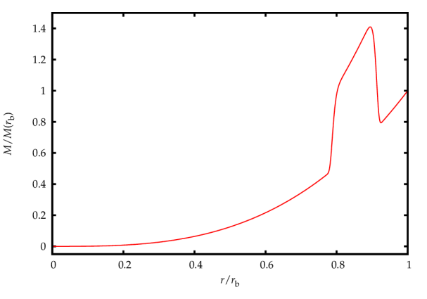
We restrict to the LTB subcase, $\mathscr{E}^{\prime}=0$, and consider the simplest possibility, where $R^{\prime}$ has one maximum at $r=r_{1}$ and one minimum at $r=r_{2}>r_{1}$. We thus have $R^{\prime}>0$ for $0\leq r<r_{1}$ and $r>r_{2}$ and $R^{\prime}<0$ for $r_{1}<r<r_{2}$. (The proper radius $R_{\mathrm{p}}$ and the proper volume (2.13) are monotonic in $r$.) Equation (2.6) shows that $M^{\prime}$ has zeroes at the same values of $r$ as $R^{\prime}$, so $M^{\prime}$ is negative for $r_{1}<r<r_{2}$. Nevertheless, the energy density integrated over the proper volume is monotonic in $r$. The function $M=4\pi\int\mathrm{d}rR^{\prime}R^{2}\rho_{\mathrm{m}}$ differs from the volume integral of the energy density by the absence of $1/\sqrt{1+E}$ in the integrand and, more importantly, the substitution of $R^{\prime}$ for $|R^{\prime}|$. The function $M(r)$ is the effective (or active) gravitating mass, which generates the gravitational field [54] (page 298), [57], and there is no physical reason for it not to decrease with radius. In fact, $\rho_{\mathrm{m}}\geq 0$ does not even rule out $M<0$, though we will have $M\geq 0$ everywhere ($M<0$ would imply $\ddot{R}>0$). For discussion of mass in general relativity in a static setting, see [74].

(a)

(b)

Figure 1: a) The function $E(r)$. b) The function $M(r)$ divided by its value on the boundary, $M(r_{\mathrm{b}})$.

(a)

(b)

(c)

(d)

Figure 2: a) The areal radius relative to the background value, $R/(ar)$. b) The local expansion rate normalised to the background expansion rate, $\theta/(3H)$. c) The shear scalar normalised to the background expansion rate, $\sigma/H$. d) The energy density normalised to the background energy density, $\rho_{\mathrm{m}}/\rho_{\mathrm{mb}}$.

With a non-monotonic $R^{\prime}$, the condition $|E|\ll 1$ is no longer required to avoid early shell crossing or collapse. Nevertheless, $E(r)\gtrsim 1$ implies $R(t_{0},r)\gtrsim(t_{0}/r_{\mathrm{b}})\sqrt{E(r)}R(t_{0},r_{\mathrm{b}})\gg R(t_{0},r_{\mathrm{b}})$ via (2.18), so the discrepancy between the volume of the hole and the region it displaces is more extreme than in the case $E\ll 1$. In the case $E(r)<0$, $|E(r)|\sim 1$, we have the constraint $M(r)\gtrsim\epsilon^{-3}M(r_{b})$. To avoid late-time apparent horizons, the condition for which is $R=2M$ [54] (page 311), there must be a similarly drastic difference in the values of $R$ inside and outside. We consider only the case $E\geq 0$ and keep $E\ll 1$. We take a spatially flat background, so the cheese consists of the EdS model. We are free to choose the three functions $M(r)$, $E(r)$ and ${t_{\mathrm{B}}}(r)$. We take ${t_{\mathrm{B}}}(r)=0$, so at early times the hole is close to the FRW background [75]. Otherwise, we do not attempt to make the holes realistic. For $M(r)$ we choose

$$M(r)=\frac{1}{2}H_{0}^{2}r^{3}\big{[}1+e^{-\left(\frac{r-r_{\mathrm{peak}}}{Ar_{\mathrm{b}}}\right)^{10}}\big{]}\ ,$$ (3.1)

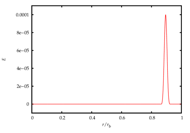
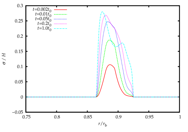
where $r_{\mathrm{peak}}=0.85r_{\mathrm{b}}$ and $A=10^{-1.2}$. The large power of $r$ in the exponent is chosen to damp the tail, so that the junction conditions are satisfied with good numerical accuracy at $r=r_{\mathrm{b}}$. The function $M(r)$ has extrema at $r_{1}=0.89r_{\mathrm{b}}$ and $r_{2}=0.92r_{\mathrm{b}}$. In this case, the condition for no shell crossings reduces to the requirement that $E^{\prime}=0$ at $r=r_{1}$ and $\mathrm{sign}(E^{\prime})\mathrm{sign}(M^{\prime})\geq 0$ elsewhere. For $E(r)$, we choose a cubic spline that is symmetric about a maximum at $r_{1}=0.89r_{\mathrm{b}}$ and has $E(r_{2})=0$. The functions $E$ and $M$ are shown in figure 1. As discussed in section 2, there are surface layers at $r=r_{i}$.

Figure 3: The spatial curvature normalised to the background expansion rate, ${{}^{(3)}R}/H^{2}$.

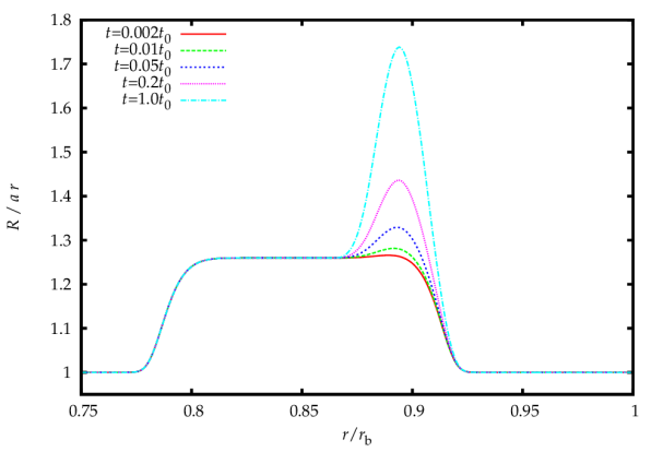
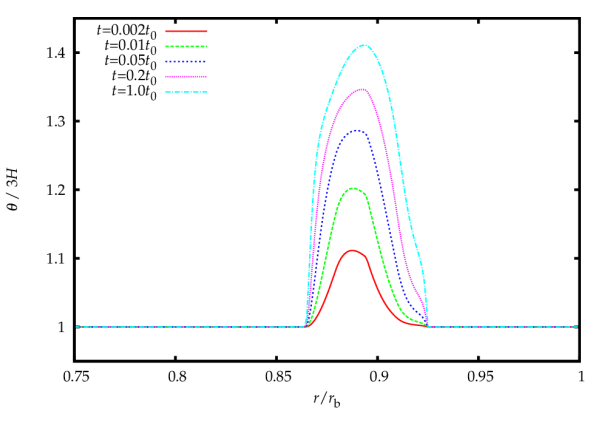
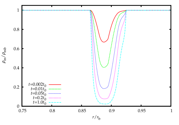
In figure 2 we show the areal radius, expansion rate, shear scalar and energy density as a function of $r$ at different times. The maximum value of the areal radius inside the hole reaches about 1.7 times the background value, the minimum of the density drops to less than 3% of the background value, and the maximum of the expansion rate grows to about 1.4 times the background value. At early times, $\theta$, $\sigma$ and $\rho_{\mathrm{m}}$ asymptotically approach their FRW values.

The model is free of shell crossings at all times. Because $R^{\prime}$ changes sign, the areal radius inside the hole can grow larger than the areal radius at the boundary, so it is possible for shells to expand fast without colliding with the boundary. The proper volume (2.13) of the hole is

$$V(t,r_{\mathrm{b}}) \simeq \frac{4\pi}{3}\left[R_{\mathrm{b}}^{3}+2R_{1}^{3}-2R_{2}^{3}\right]\ ,$$ (3.2)

where we have denoted $R_{\mathrm{b}}\equiv R(t,r_{\mathrm{b}}),R_{i}\equiv R(t,r_{i})$. As $R_{1}>R_{2}$, the volume is larger than in the FRW case, and the average expansion (from (2.1) and (2.14)) is correspondingly faster:

$$\langle{\theta}\rangle \simeq 3H\frac{1+2\frac{\dot{R}_{1}}{R_{1}}\left(\frac{R_{1}}{R_{\mathrm{b}}}\right)^{3}-2\frac{\dot{R}_{2}}{R_{2}}\left(\frac{R_{2}}{R_{\mathrm{b}}}\right)^{3}}{1+2\left(\frac{R_{1}}{R_{\mathrm{b}}}\right)^{3}-2\left(\frac{R_{2}}{R_{\mathrm{b}}}\right)^{3}}\ .$$ (3.3)

The average spatial curvature and the average energy density are, from (2.6), (2.1) and (2.14),

$$\langle{{{}^{(3)}R}}\rangle \simeq -2\frac{\int_{0}^{r_{\mathrm{b}}}\mathrm{d}r\frac{|R^{\prime}|}{R^{\prime}}(ER)^{\prime}}{\int_{0}^{r_{\mathrm{b}}}\mathrm{d}r|R^{\prime}|R^{2}}=-6\frac{E_{1}R_{1}}{R_{\mathrm{b}}^{3}+2R_{1}^{3}-2R_{2}^{3}}$$

$$\langle{\rho_{\mathrm{m}}}\rangle \simeq \frac{1}{4\pi G_{\mathrm{N}}}\frac{\int_{0}^{r_{\mathrm{b}}}\mathrm{d}r|M^{\prime}|}{\int_{0}^{r_{\mathrm{b}}}\mathrm{d}r|R^{\prime}|R^{2}}=\frac{3}{4\pi G_{\mathrm{N}}}\frac{M_{\mathrm{b}}+2M_{1}-2M_{2}}{R_{\mathrm{b}}^{3}+2R_{1}^{3}-2R_{2}^{3}}\ ,$$ (3.4)

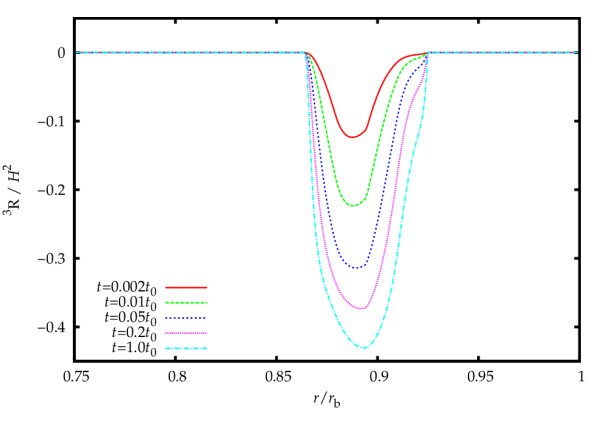
where $E_{i}\equiv E(r_{i}),M_{i}\equiv M(r_{i}),M_{\mathrm{b}}\equiv M(r_{\mathrm{b}})$ and we have taken into account that absence of singularities requires $E(0)=0,M(0)=0$. Note that $|E|\ll 1$ does not imply that the spatial curvature would be small either locally or on average. The spatial curvature is shown in figure 3. For our choices of $E$ and $M$, the spatial curvature does not approach its FRW value even at early times, unlike the expansion rate, shear and energy density.

Inner and outer size.

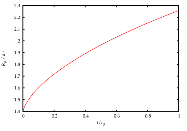
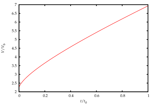
We have removed a portion of spacetime and fitted in its place another region that fits smoothly into the hole on the boundary, but has larger spatial volume than the removed part. We call a solution that features one or more such domains whose inner dimensions seem at odds with the outer a Tardis spacetime, and refer to the embedded domains as Tardis regions. A Tardis region can be much larger than expected from its surface area and the linear size it occupies in the background spacetime based on Euclidean intuition. (Note that the surface layer is located inside the Tardis region, and the interface between the Tardis region and the outside world appears normal.) The proper radius and proper volume of the hole relative to the background are shown in figure 4. The proper radius is today about 2 times as large as that of the removed region, and the proper volume is about 7 times as large. The relation $\langle{\theta}\rangle=\dot{V}/V$ implies that if the average expansion rate is different from the background (and monotonic), the volume element will also be different, but the reverse does not hold true. At early times, the average expansion rate is close to FRW, but the proper radius and proper volume do not approach their FRW values, as $R$ is discontinuous at all times. It would be possible to tune the function $M(r)$ so that the volume of the hole is close to the background at early times, but this is not a necessary consequence of time evolution, unlike for the expansion rate, shear and energy density.

(a)

(b)

Figure 4: a) Proper radius relative to a background region with the same areal radius, $R_{\mathrm{p}}/(ar)$. b) Proper volume relative to the volume of a background region with the same areal radius, $V/V_{b}$.

As the volume element is defined locally, its values inside a given volume are not determined by the values on the boundary. We have defined the Tardis region in terms of embedding into a background spacetime, so the volume of the embedded region can be compared with the corresponding background region. A realistic model would not consist of isolated regions embedded in a homogeneous and isotropic background that provides a global point of comparison. Nevertheless, the Tardis effect is central to general relativity and can be formulated without reference to embedding. Consider a spherical region (i.e. a simply connected volume such that all points on the boundary are at the same proper distance from one point) in any three-dimensional curved space and define the areal radius by $R\equiv\sqrt{S/(4\pi)}$, where $S$ is the area of the boundary. In general, the proper radius of the sphere is not $R$ and its volume is not $4\pi R^{3}/3$. A well-known example is given by spatially curved FRW models. In the real universe, underdense regions with negative curvature are in this sense larger than expected, and overdense regions correspondingly smaller (neglecting factors such as shear and rotation).

Figure 5: The fraction of volume taken up by the holes, as a function of the mean redshift (3.25).

Cosmological model.

We construct a cosmological model with a distribution of time evolving underdense Tardis regions. In the real universe voids, underdense regions which expand faster than average, are a central feature of the observed matter distribution. The void distribution is dominated by voids of a certain size, whose evolution is governed by the power spectrum of perturbations. Typical void radius today is of the order 20 Mpc $\sim 10^{-2}H_{0}^{-1}$ [76]. We consider holes that are all identical to each other, with comoving areal radius $r_{\mathrm{b}}=0.01H_{0}^{-1}$, so that their outer size is similar to that of real structures, though their density profile (shown in figure 2) is not realistic. Real cosmological structures have a complex multiscale arrangement of clusters, filaments and walls in addition to voids [77], and modelling this accurately would require dealing with the statistics of hierarchical structure formation.

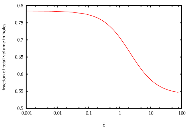
We distribute voids randomly in the background space with a uniform distribution, and remove overlapping regions. The voids take up about 34% of the volume as measured by their “outer size”, i.e. the size of the FRW regions they displace. As the volume of the voids grows faster than the background, their fraction of the real volume increases in time, as shown in figure 5.

3.2 Light propagation

Redshift, angular diameter distance and null shear.

We consider light propagation in the geometrical optics approximation, so light travels on null geodesics [78] (page 93), [79]. Photon momentum, which is tangent to the null geodesic, is denoted by $k^{\alpha}=\frac{\mathrm{d}x^{\alpha}}{\mathrm{d}\lambda}$, where $\lambda$ is the affine parameter. Redshift measured by an observer comoving with the dust is given by the ratio of the energy $E_{\mathrm{s}}$ emitted at the source and the observed energy $E_{\mathrm{o}}$,

$$1+z = \frac{E_{\mathrm{s}}}{E_{\mathrm{o}}}=\frac{k^{0}}{k^{0}_{\mathrm{o}}}\ ,$$ (3.5)

where we have used $E=-u_{\alpha}k^{\alpha}=k^{0}$. We decompose $k^{\alpha}$ into an amplitude and the direction, and split the direction into components orthogonal and parallel to the dust geodesics,

$$k^{\alpha}=E(u^{\alpha}+e^{\alpha})\ ,$$ (3.6)

where $u_{\alpha}e^{\alpha}=0$, $e_{\alpha}e^{\alpha}=1$. In terms of the covariant quantities (2.1), the redshift is (see e.g. [22])

$$1+z = \exp\left(\int_{\lambda_{\mathrm{s}}}^{\lambda_{\mathrm{o}}}\mathrm{d}\lambda E\left[\frac{1}{3}\theta+\sigma_{\alpha\beta}e^{\alpha}e^{\beta}\right]\right)\ .$$ (3.7)

Because of spherical symmetry we can restrict our consideration to the hypersurface $\theta=\pi/2$ without loss of generality, so $k^{\theta}=0$. The other components $k^{\alpha}$ can be solved from the null condition $k_{\alpha}k^{\alpha}=0$ and the null geodesic equation $k^{\beta}\nabla_{\beta}k^{\alpha}=0$. From the $\phi$-component of the latter we get $k^{\phi}=c_{\phi}/R^{2}$, where $c_{\phi}$ is a constant. Defining the Euclidean impact parameter as $b\equiv r_{\mathrm{min}}^{E}/r_{\mathrm{b}}$, where $r_{\mathrm{min}}^{E}$ is the smallest $r$-coordinate the light ray would have were the space Euclidean, we have $c_{\phi}=br_{\mathrm{b}}$. The other components of the null geodesic equation give

$$\frac{\mathrm{d}k^{0}}{\mathrm{d}\lambda}+\frac{\dot{R}^{\prime}}{R^{\prime}}(k^{0})^{2}+\left(\frac{\dot{R}}{R}-\frac{\dot{R}^{\prime}}{R^{\prime}}\right)\frac{c_{\phi}^{2}}{R^{2}} = 0$$ (3.8)

$$\frac{\mathrm{d}(Xk^{r})}{\mathrm{d}\lambda}+\frac{\dot{R}^{\prime}}{R^{\prime}}k^{0}Xk^{r}-\frac{1}{X}\frac{R^{\prime}}{R}\frac{c_{\phi}^{2}}{R^{2}} = 0\ .$$ (3.9)

The component $k^{r}$ generally diverges when $X=0$, but $Xk^{r}$ remains finite. However, the derivative $\frac{\mathrm{d}(Xk^{r})}{\mathrm{d}\lambda}$ jumps because of the absolute value structure of $R^{\prime}/X$ in the last term in (3.9). Correspondingly, the derivative of $k^{\phi}$ jumps, as the components are related by the null condition,

$$Xk^{r}=\pm\sqrt{(k^{0})^{2}-\frac{c_{\phi}^{2}}{R^{2}}}\ .$$ (3.10)

The area and shape of a bundle of null geodesics are solved from the Sachs equations:

$$\frac{\mathrm{d}{\tilde{\theta}}}{\mathrm{d}\lambda}+\frac{1}{2}\tilde{\theta}^{2}+2\tilde{\sigma}^{2} = -G_{\alpha\beta}k^{\alpha}k^{\beta}$$

$$\tilde{h}_{\alpha}^{\ \ \gamma}\tilde{h}_{\beta}^{\ \ \delta}\frac{\mathrm{d}{\tilde{\sigma}_{\gamma\delta}}}{\mathrm{d}\lambda}+\tilde{\theta}\tilde{\sigma}_{\alpha\beta} = -k^{\mu}k^{\nu}\tilde{h}_{\alpha}^{\ \ \gamma}\tilde{h}_{\beta}^{\ \ \delta}C_{\mu\gamma\nu\delta}\ ,$$ (3.11)

where $\tilde{\theta}\equiv\nabla_{\alpha}k^{\alpha}$ is the area expansion rate of the light bundle, $\tilde{\sigma}_{\alpha\beta}\equiv\tilde{h}_{\alpha}^{\ \ \gamma}\tilde{h}_{\beta}^{\ \ \delta}\nabla_{\delta}k_{\gamma}-\frac{1}{2}\tilde{h}_{\alpha\beta}\tilde{\theta}$ is the null shear tensor which describes image deformation, $\tilde{\sigma}\equiv\sqrt{\frac{1}{2}\tilde{\sigma}_{\alpha\beta}\tilde{\sigma}^{\alpha\beta}}$ is the null shear scalar, $\tilde{h}_{\alpha\beta}$ projects on a two-dimensional surface orthogonal to the light ray and $C_{\alpha\beta\gamma\delta}$ is the Weyl tensor. The quantities $\tilde{\theta}$ and $\tilde{\sigma}$ are independent of the choice of $\tilde{h}_{\alpha\beta}$.

The tensors $G_{\alpha\beta}$ and $C_{\alpha\beta\gamma\delta}$ have delta functions in the shells where $X=0$, coming from terms of the form $X^{\prime}/X$. Exactly the same delta functions appear on the left-hand side in $\frac{\mathrm{d}{\tilde{\theta}}}{\mathrm{d}\lambda}$ and $\frac{\mathrm{d}{\tilde{\sigma}_{\alpha\beta}}}{\mathrm{d}\lambda}$, so the delta function parts of the equations are satisfied identically, and we drop them in what follows. Because of spherical symmetry, $\tilde{\sigma}_{\alpha\beta}$ has only one independent component, which we can express in terms of $\tilde{\sigma}$. For the LTB metric given by (2.2) and (2.3), the smooth parts of the Sachs equations (3.2) reduce to

$$\frac{\mathrm{d}{\tilde{\theta}}}{\mathrm{d}\lambda}+\frac{1}{2}\tilde{\theta}^{2}+2\tilde{\sigma}^{2} = -8\pi G_{\mathrm{N}}\rho_{\mathrm{m}}(k^{0})^{2}$$ (3.12)

$$\frac{\mathrm{d}{\tilde{\sigma}}}{\mathrm{d}\lambda}+\tilde{\theta}\tilde{\sigma} = \frac{c_{\phi}}{R^{2}}\left(4\pi G_{\mathrm{N}}\rho_{\mathrm{m}}-3\frac{M}{R^{3}}\right)\ ,$$ (3.13)

where we have used the Einstein equation (2.1). The area expansion rate is related to the angular diameter distance by $D_{A}\propto\exp\left({\frac{1}{2}\int\mathrm{d}\lambda\tilde{\theta}}\right)$. For an observer located in the centre, we would simply have $\tilde{\sigma}=0$ and $D_{A}=R$. In terms of $D_{\mathrm{A}}$, (3.12) reads

$$\frac{\mathrm{d}^{2}D_{A}}{\mathrm{d}\lambda^{2}} = -[4\pi G_{\mathrm{N}}\rho_{\mathrm{m}}(k^{0})^{2}+\tilde{\sigma}^{2}]D_{A}\ .$$ (3.14)

The sources on the right-hand side of the Sachs equations (3.12) and (3.13) are continuous. Therefore the equations have solutions that are continuous; however, the solutions that correspond to the spacetime with surface layers are those in which $\tilde{\theta}$ and $\tilde{\sigma}$ and their first derivatives have finite discontinuities at the locations where $X=0$. The magnitude of the jumps is given by the inverse size of the hole, so for one hole the relative change is of order unity. When travelling cosmological distances, the relevant scale for $\tilde{\theta}$ is $H$, so the jumps are much larger than the continuous part. In other words, the surface layers completely distort light propagation compared to the smooth case. It is also not clear whether the geometrical optics approximation holds, as the curvature changes on an infinitely small scale when crossing surface layers; the issue would have to be settled by studying the thin limit of a thick shell.

We consider two modified versions of the light propagation calculation. In the first case, we still calculate the photon momentum from the null geodesic equation but modify the distance calculation by picking the continuous solutions of the Sachs equations (3.12) and (3.13) instead of the discontinuous solutions. This corresponds to angular diameter distance in a spacetime without the surface layers. The absolute value structure of $X$ still has an effect on the calculation by causing a jump in $\mathrm{d}k^{\phi}/\mathrm{d}\lambda$ according to the null geodesic equation (3.9). This makes the light ray turn sharply when it crosses a surface layer. In order to assess the importance of this effect on the redshift, we consider a second modification of light propagation, in which we take the light rays to follow straight null lines as defined by the background metric and calculate the redshift from (3.7). This removes light deflection due to the unphysical surface layers. (In solutions without surface layers, there would of course still be some light deflection, but it would be small.) However, these straight null rays are no longer geodesic, so the Sachs equations do not hold and it is not meaningful to calculate the angular diameter distance along them, so in the second case we consider only the redshift.

Light propagation calculation.

We consider an octant of a ball with radius $60r_{\mathrm{b}}$ centered on the observer, and fill it with voids drawn from a uniform distribution, removing overlapping spheres. Beyond this region we generate the distribution of voids dynamically along the null geodesic in order to cut down on computation time. We integrate from the observer to the source, and stop the calculation when we reach time $t=2\times 10^{-3}t_{0}$. A typical light ray goes through approximately $35\pm 5$ holes for the case when the light rays are geodesic, and $40\pm 5$ when they go straight as defined by the background. We propagate the null shear consistently using the Sachs equations, using the same procedure as in [34], which presented the first correct treatment of the shear in Swiss Cheese models (in the prescription in which the light rays are propagated from the observer to the source, as is common in the literature). As in [34], the null shear is small, its contribution relative to the density in (3.14) is at most $10^{-3}$.

Equation (3.14) is linear, so the normalisation of $D_{A}$ is arbitrary. In the FRW model, the normalisation is fixed and for small redshifts we have $D_{A}\simeq H_{0}^{-1}z$, where $H_{0}$ is the current value of the Hubble parameter. When the expansion rate is inhomogeneous, as in our model and in the real universe, the correct normalisation is less clear. The naive idea of using the volume expansion rate at the observer’s location is inappropriate. For an observer located in a stable object such as a galaxy, the local expansion rate is zero, and for an observer located in a collapsing region it is negative. The choice of normalisation should be related to how real observations are analysed. In practice, the value of $H_{0}$ that is used is a weighted average over some redshift range. For example, the determination of $H_{0}$ in [80] uses data in the ranges $0.023<z<0.1$ and $0.01<z<0.1$. On the theoretical side, the issue has been discussed in [50, 81]. We normalise to the spatially averaged value of the volume expansion rate, as also done in [24]. Let us discuss spatial averages in more detail before showing the results of the light propagation calculation and commenting on how well the redshift and the distance are described by the average expansion rate.

3.3 Average quantities

The average expansion rate.

As discussed in section 1, it has been suggested that light propagation in a statistically homogeneous and isotropic space in which the distribution evolves slowly can be described in terms of the average expansion rate [18, 29, 22, 23, 24]. We can now test this idea with our Swiss Cheese model.

The evolution and constraint equations for a general geometry can be written in terms of the covariant quantities (2.1). For a general irrotational dust model, the scalar parts are [60, 61, 62, 63, 64]

$$\dot{\theta}+\frac{1}{3}\theta^{2} = -4\pi G_{\mathrm{N}}\rho_{\mathrm{m}}-2\sigma^{2}$$ (3.15)

$$\frac{1}{3}\theta^{2} = 8\pi G_{\mathrm{N}}\rho_{\mathrm{m}}-\frac{1}{2}{{}^{(3)}R}+\sigma^{2}$$ (3.16)

$$0 = \dot{\rho}_{\mathrm{m}}+\theta\rho_{\mathrm{m}}\ .$$ (3.17)

In the present case, there are surface layers in addition to dust. Equation (2.1) shows that $\theta$ and $\sigma$ are smooth everywhere. In contrast, ${{}^{(3)}R}$ has a delta function contribution at the locations where $R^{\prime}=0$, as discussed in section 2. We have not written down the surface layer contribution to the spatial curvature in (3.16), as it is exactly cancelled by the energy density of the surface layer.

The scale factor $\bar{a}(t)$ that describes the evolution of the proper volume (not to be confused with the background scale factor $a(t)$) is defined as

$$\bar{a}(t)\equiv\left(\frac{V(t)}{V(t_{0})}\right)^{\frac{1}{3}}\ ,$$ (3.18)

and the average Hubble parameter is defined as $\bar{H}\equiv\dot{\bar{a}}/\bar{a}$, or equivalently as $3\bar{H}=\langle{\theta}\rangle$. Averaging (3.15)-(3.17) over the hypersurface of constant $t$, we obtain the Buchert equations [6] that describe the evolution of $\bar{a}$:

$$3\frac{\ddot{\bar{a}}}{\bar{a}} = -4\pi G_{\mathrm{N}}\langle{\rho_{\mathrm{m}}}\rangle+\mathcal{Q}$$ (3.19)

$$3\frac{\dot{\bar{a}}^{2}}{\bar{a}^{2}} = 8\pi G_{\mathrm{N}}\langle{\rho_{\mathrm{m}}}\rangle-\frac{1}{2}\langle{{{}^{(3)}R}}\rangle-\frac{1}{2}\mathcal{Q}$$ (3.20)

$$0 = \partial_{t}\langle{\rho_{\mathrm{m}}}\rangle+3\frac{\dot{\bar{a}}}{\bar{a}}\langle{\rho_{\mathrm{m}}}\rangle\ ,$$ (3.21)

where the backreaction variable is defined as $\mathcal{Q}\equiv\frac{2}{3}\left(\langle{\theta^{2}}\rangle-\langle{\theta}\rangle^{2}\right)-2\langle{\sigma^{2}}\rangle$. The integrability condition between (3.19) and (3.20) is

$$\partial_{t}\langle{{{}^{(3)}R}}\rangle+2\bar{H}\langle{{{}^{(3)}R}}\rangle=-\dot{\mathcal{Q}}-6\bar{H}\mathcal{Q}\ .$$ (3.22)

Dividing (3.19) and (3.20) by $3\bar{H}^{2}$, we get [6]

$$q_{H} \equiv -\frac{1}{\bar{H}^{2}}\frac{\ddot{\bar{a}}}{\bar{a}}=\frac{1}{2}\Omega_{\mathrm{m}}+2\Omega_{\mathcal{Q}}$$ (3.23)

$$1 = \Omega_{\mathrm{m}}+\Omega_{R}+\Omega_{\mathcal{Q}}\ ,$$ (3.24)

where $\Omega_{\mathrm{m}}\equiv 8\pi G_{N}\langle{\rho_{\mathrm{m}}}\rangle/(3\bar{H}^{2})$, $\Omega_{R}\equiv-\langle{{{}^{(3)}R}}\rangle/(6\bar{H}^{2})$ and $\Omega_{\mathcal{Q}}\equiv-\mathcal{Q}/(6\bar{H}^{2})$ are the density parameters of matter, spatial curvature and the backreaction variable, respectively.

(a)

(b)

Figure 6: a) The average expansion rate times the age of the universe, $\bar{H}t$, as a function of the mean redshift (3.25). b) The deceleration parameters $q_{H}$ and $q_{D}$ as a function of the the mean redshift (3.25). The quantity $q_{D}$ corresponding to the physical distance is shown as a function of the physical redshift instead; see section 3.5.

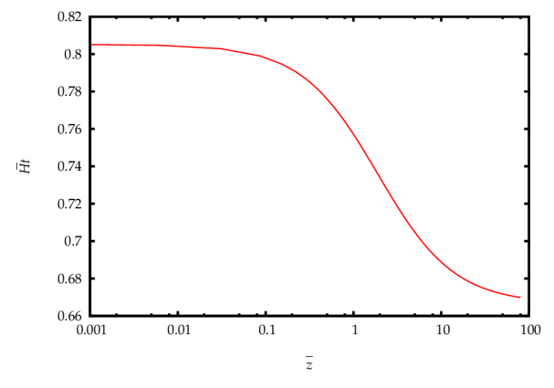
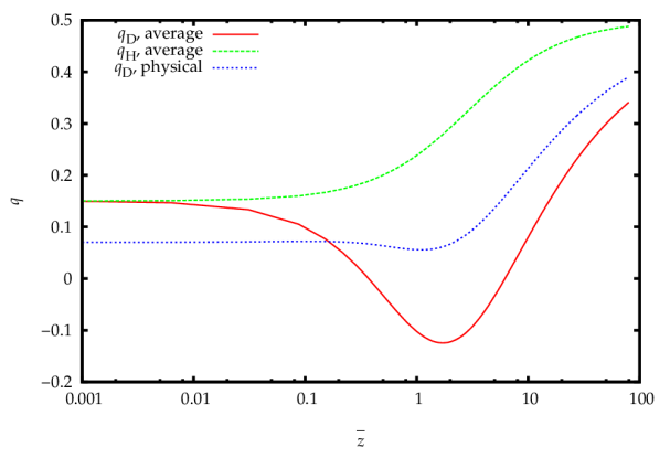
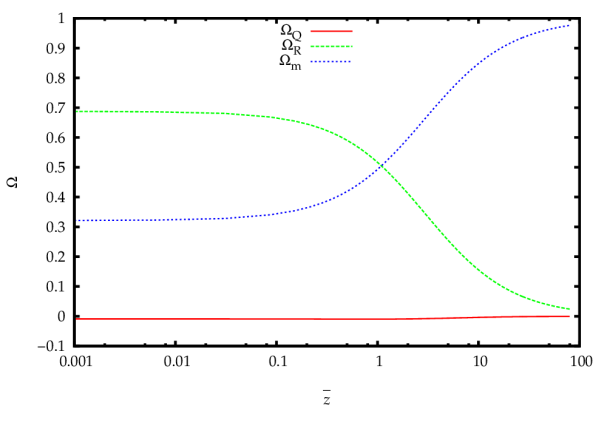
The average expansion rate times the age of the universe, $\bar{H}t$, is shown in figure 6a as a function of the mean redshift $\bar{z}$ (defined below in (3.25)). At large redshifts (corresponding to early times), the average expansion rate is close to the EdS case, but at redshifts of order unity and smaller the holes expand significantly faster than the background, so $\bar{H}t$ grows. In a universe completely dominated by completely empty voids, we would have $\bar{H}t=1$. Note that the average expansion rate only decelerates less, it does not accelerate. The corresponding deceleration parameter $q_{H}$ is shown in figure 6b, and it is positive at all times. (We also show the deceleration parameters $q_{D}$ that correspond to the distance instead of the average expansion rate; see section 3.5.) The density parameters are shown in figure 7.

Figure 7: The density parameters $\Omega_{\mathrm{m}}$, $\Omega_{R}$ and $\Omega_{\mathcal{Q}}$ as a function of the mean redshift (3.25).

The values today are $\Omega_{\mathrm{m0}}=0.32,\Omega_{R0}=0.69$ and $\Omega_{\mathcal{Q}0}=-0.01$. The backreaction variable is small at all times, $|\Omega_{\mathcal{Q}}|\lesssim 0.01$. This does not mean that inhomogeneities have a small effect on the expansion rate, just that the effect reduces to a spatial curvature term that evolves like $\propto\bar{a}^{-2}$, i.e. in the same way as in the FRW case [82, 83, 29].

Mean redshift and angular diameter distance.

In [22, 23] it was argued that in a statistically homogeneous and isotropic dust universe in which the distribution evolves slowly, the redshift is approximately equal to the mean redshift over distances larger than the homogeneity scale,

$$1+\bar{z}\equiv\bar{a}(t)^{-1}=e^{\int_{t}^{t_{0}}\mathrm{d}t^{\prime}\bar{H}(t^{\prime})}\ ,$$ (3.25)

and the angular diameter distance can to first approximation be solved from

$$\bar{H}\frac{\mathrm{d}}{\mathrm{d}\bar{z}}\left[(1+\bar{z})^{2}\bar{H}\frac{\mathrm{d}D_{A}}{\mathrm{d}\bar{z}}\right] = -4\pi G_{\mathrm{N}}\langle{\rho_{\mathrm{m}}}\rangle D_{A}\ ,$$ (3.26)

where $4\pi G_{\mathrm{N}}\langle{\rho_{\mathrm{m}}}\rangle=\frac{3}{2}\Omega_{\mathrm{m0}}\bar{H}_{0}^{2}(1+\bar{z})^{3}$ due to (3.21) and (3.25). The equation (3.26) determines the distance, given $\bar{H}(\bar{z})$ and $\Omega_{\mathrm{m0}}$. The luminosity distance is $D_{L}(\bar{z})=(1+\bar{z})^{2}D_{A}(\bar{z})$ [84, 61]. The quantities calculated from (3.25) and (3.26) are mean values, with small variations expected for typical light rays, and possibly large variations for exceptional lines of sight, e.g. in the case of strong lensing.

3.4 Averages and light propagation

(a)

(b)

Figure 8: a) The angular diameter distance calculated from the light propagation equations, from the average expansion rate and in the background model. For the physical distance the error bars show standard deviation for 1000 light rays, and the line shows an FRW model that gives a good fit. Distance in the spatially flat $\Lambda$CDM model with the same $\Omega_{\mathrm{m0}}=0.32$ as in the physical model is also shown for comparison. b) The relative difference of the angular diameter distance corresponding to the best-fit FRW model and the angular diameter distance calculated from the average expansion rate.

Angular diameter distance.

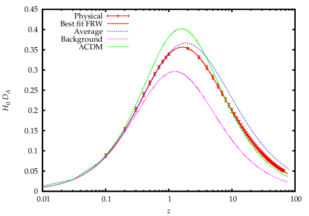
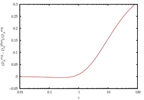
Let us now see how well the mean quantities calculated from (3.25) and (3.26) describe the redshift and the angular diameter distance calculated with the light propagation equations, as discussed in section 3.2. In figure 8 we compare the distance calculated from the null geodesic equation and the Sachs equations as a function of the physical redshift, the mean distance calculated from from the average expansion rate using (3.26) as a function of the mean redshift (3.25), and the background distance as a function of the background redshift $1+z_{\mathrm{b}}=a(t)^{-1}$. The distance-redshift relation of the $\Lambda$CDM model with the same $\Omega_{\mathrm{m0}}=0.32$ as the Swiss Cheese model is also shown for comparison.

The physical distance is very different from the background distance. It is also slightly different for different light rays. We have propagated 1000 light rays and fit a FRW model with dust, spatial curvature and vacuum energy to the resulting points. A model with $\Omega_{\mathrm{m0}}=0.42$, $\Omega_{K0}=0.44$ and $\Omega_{\Lambda 0}=0.14$ gives an excellent description of the physical distance. The distance calculated from the average expansion rate also gives a reasonable description of the physical distance up to $z\approx 1$, but for higher redshifts the agreement is rather poor. At $z=100$ the distance calculated from the average expansion rate overestimates the real distance by more than 30%. The discrepancy is related to the fact that the integrated expansion rate and density along a light ray are different from the average quantities. Looking at the redshift will show this in more detail.

Redshift.

(a)

(b)

(c)

(d)

Figure 9: a) The relative difference to the background redshift for the redshift calculated from the null geodesic equation and the mean redshift calculated from the average expansion rate. The error bars show the standard deviation for 1000 light rays. b) The relative difference between the redshift calculated from the null geodesic equation and the mean redshift. c) The same as a), but with the redshift calculated along null curves that are straight relative to the background instead of using the null geodesic equation. d) The same as b), but with the redshift calculated along null curves that are straight relative to the background instead of using the null geodesic equation.

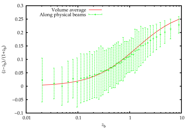
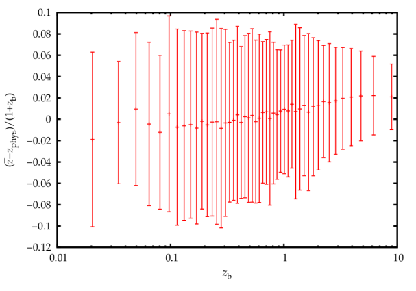
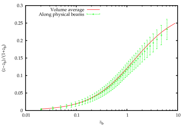
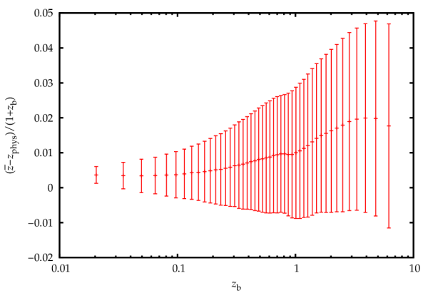
We consider the redshift calculated from the null geodesic equations without change, as well as a modified redshift calculated from null curves that are straight according to the background metric. In figure 9a we show the relative deviation from the background for the redshift calculated from the null geodesic equation as well as for the mean redshift $\bar{z}$. In figure 9b we show the relative difference between the physical redshift and the mean redshift. As with the distance, the physical redshift is quite different from the background redshift, and the difference grows monotonically. The reason is that the expansion rate (and the shear) along the light ray are different from the background expansion rate. The mean redshift (3.25) calculated from the average expansion rate has the same systematic evolution as the physical redshift, with statistical deviations of order 10% for small redshifts and 5% for high redshifts. There appears to be a small systematic offset at large redshifts, though it should be noted that as the bins are equally spaced in time, the largest redshifts are sparsely sampled. In figures 9c and 9d we show the same comparison for the redshift calculated along null curves that are straight according to the background metric, i.e. with the sharp turns due to the surface layers neglected. In this case, the mean redshift agrees with the physical redshift even better, with a statistical error of less than 5% at all redshifts, showing that most of the discrepancy between the physical redshift and the mean redshift in the full case is due to the surface layers.

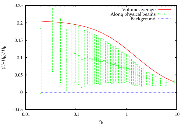
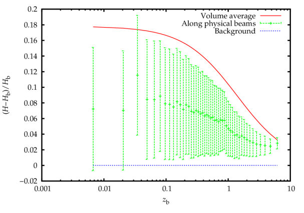
It is notable that in neither case is the mean expansion rate along the light ray the same as the spatial average. In figure 10 we show the relative deviation from the background expansion rate for the expansion rate along the light ray and the spatial average of the expansion rate. For both treatments of the physical redshift, the expansion rate seen by the light rays is between the background value and the spatial average. This is also true for the energy density.

(a)

(b)

Figure 10: a) The relative difference from the background expansion rate for the expansion rate along the light ray and the the spatial average of the expansion rate. The error bars show the standard deviation for 1000 light rays. b) The same plot for the case when the light rays go straight according to the background metric.

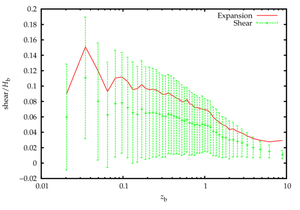
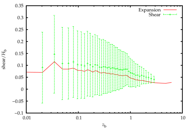
In [22, 23] it was argued that the mean expansion rate along a light ray and the spatial average of the expansion rate should be close to each other for slowly evolving and small structures with a statistically homogeneous and isotropic distribution. The argument was that in the integral (3.7), one would the contributions of $\frac{1}{3}\Delta\theta\equiv\frac{1}{3}\left(\theta-\langle{\theta}\rangle\right)$ and $\sigma_{\alpha\beta}e^{\alpha}e^{\beta}$ to be highly suppressed for symmetry reasons. In the present case, these two terms cancel each other, as in the near-FRW case [25], but they do not cancel individually. The expansion rate seen by a typical light ray is quite different from the spatially averaged expansion rate, but this difference cancels with the shear to leave only the contribution of the average expansion rate. The importance of the shear can be seen in figure 11, which shows that the shear is comparable to the deviation of the expansion rate along the null geodesic from the background expansion rate. This is unexpected, and it would be interesting to repeat the analysis in an exact solution that does not have surface layers.

(a)

(b)

Figure 11: a) The shear normalised to the background expansion rate, $\sigma_{\alpha\beta}e^{\alpha}e^{\beta}/H$, along the null geodesic. The error bars show the standard deviation for 1000 light rays. The red line shows the relative deviation of the expansion rate along the line of sight from the background expansion rate (i.e. the quantity plotted in figure 9), without error bars. b) The same plot for the case when the light rays go straight according to the background metric.

3.5 Signatures of backreaction

FRW consistency parameters.

If backreaction is significant, the relation between the average expansion rate and the distance is in general different from the FRW case. This is an important aspect of backreaction, which cannot be reproduced by any model based on the four-dimensional FRW metric, regardless of the matter content or the equation of motion [22, 21].

In addition to the average expansion rate $\bar{H}$ that describes how the volume of the universe evolves, it is useful to define a ’fitting’ expansion rate $H_{\mathrm{fit}}$ that describes how the distance evolves [21]. Specifically, $H_{\mathrm{fit}}(z)$ is the expansion rate of the spatially flat FRW “fitting model” that has the same distance-redshift relation $D_{A}(z)$ as the backreaction model. In a FRW model, the angular diameter distance is

$$D_{A}(z)=(1+z)^{-1}\frac{1}{\sqrt{-K}}\sinh\left(\sqrt{-K}\int_{0}^{z}\frac{\mathrm{d}\tilde{z}}{H(\tilde{z})}\right)\ ,$$ (3.27)

where $K$ is the spatial curvature constant defined in (2.1). We thus have, defining $D\equiv(1+z)D_{A}$,

$$H_{\mathrm{fit}}(z)=\frac{1}{D^{\prime}(z)}\ ,$$ (3.28)

where the prime refers to derivative with respect to $z$, not $r$. As the distance is normalised to $D\simeq\bar{H}_{0}^{-1}z$ for $z\ll 1$, the expansion rates $H_{\mathrm{fit}}$ and $\bar{H}$ agree at small redshift, and (if backreaction is significant) disagree at large redshift.

As in [85], we can solve $K$ from (3.27) to obtain

$$K = \frac{1-(HD^{\prime})^{2}}{D^{2}}\ .$$ (3.29)

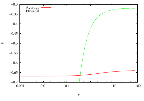
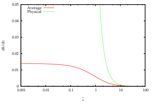
The relation (3.29) is now taken as the definition of a function $K(z)$ in the general case when the universe is not necessarily described by a FRW model, with the FRW expansion rate $H$ replaced by the average expansion rate $\bar{H}$. (In general, $K$ would also be function of angular direction, but for distances larger than the homogeneity scale the directional dependence is expected to be small if the universe is statistically homogeneous and isotropic [22, 23].) In terms of the fitting model expansion rate, we have

$$K(z) = \frac{1-\left[\bar{H}(z)/H_{\mathrm{fit}}(z)\right]^{2}}{\left[\int_{0}^{z}\mathrm{d}\tilde{z}/H_{\mathrm{fit}}(\tilde{z})\right]^{2}}\ .$$ (3.30)

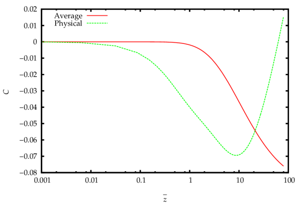
In [85], the following quantity was also introduced to quantify the deviation of $K$ from constant:

$$\mathscr{C}\equiv-\frac{D^{3}}{2D^{\prime}}K^{\prime}=1+\bar{H}^{2}(DD^{\prime\prime}-D^{\prime 2})+\bar{H}\bar{H}^{\prime}DD^{\prime}\ .$$ (3.31)

If the average expansion rate, redshift and distance are well described by the FRW model, $K$ is constant and equal to $-\bar{H}_{0}^{2}\Omega_{R0}$. Observational ranges for $K$ were determined in [86, 87], with the result $|K|/\bar{H}_{0}^{2}\lesssim 1$, though there may be significant systematic uncertainty. If $K$ is observed to vary with redshift, the universe cannot be described by any four-dimensional FRW model. On the other hand, a magnitude of $0.1\lesssim|K|/\bar{H}_{0}^{2}\lesssim 1$ is expected if backreaction is significant in the real universe and light propagation is well described by (3.25) and (3.26) [21], which is the case in our model for redshifts below unity. However, a constant $K$ does not rule out significant backreaction, because clumpiness could in principle change the expansion rate and distance in a way that preserves the FRW relation. In particular, if the average expansion rate and distance are related by (3.26) and clumpiness changes the average expansion rate by $\bar{H}(z)^{2}\rightarrow\bar{H}(z)^{2}+A+B(1+z)^{2}+C(1+z)^{3}$, where $A$, $B$ and $C$ are constants (i.e. like a mixture of dust, spatial curvature and vacuum energy in the FRW model), the relation between the expansion rate and distance is identical to the FRW case. Likewise, $K^{\prime}\neq 0$ does not necessarily indicate backreaction, as the relation between the expansion rate and the distance is also altered in models in which the universe is spherically symmetric (and inhomogeneous) on Gpc scales [88] and in some models with extra dimensions [89].

(a)

(b)

(c)

Figure 12: a) The FRW consistency parameter $k\equiv K/\bar{H}_{0}^{2}$. b) The $z$-derivative of $k$. c) The FRW consistency parameter $\mathscr{C}$.

In figure 12 we show $K$, $K^{\prime}$ and $\mathscr{C}$ both for the distance calculated from the average expansion rate using (3.25) and (3.26) and for the physical distance (more precisely, we use the FRW model that gives an excellent fit to the physical distance calculated from 1000 light rays, as discussed in section 3.4). For the average expansion rate, the quantity $K$ is almost constant, and $K^{\prime}$ and $\mathscr{C}$ are small. This corresponds to the fact that backreaction in the model changes the average expansion rate in almost the same way as FRW negative spatial curvature. The behaviour of $K$, $K^{\prime}$ and $\mathscr{C}$ is very different in the case of the physical distance. For large redshifts this is to be expected, because the two distances agree well only at $z\lesssim 1$. The discrepancy at small $z$, in turn, is related to the fact that the denominator of $K$ vanishes like $z^{2}$ at small $z$. For the distance solved from (3.26), the numerator goes to zero at the same rate, so $K$ is finite at $z=0$. However, for the physical distance the numerator only vanishes like $z$, so $K$ diverges as $1/z$ as $z$ approaches zero. From the observational point of view, the fact that an arbitrarily small mismatch between $D^{\prime}$ and $\bar{H}$ in (3.30) leads to divergent $K$ and $K^{\prime}$ means that the error bars on $K$ and $K^{\prime}$ diverge at small $z$. The consistency parameter $\mathscr{C}$ is defined in such a way that it does not diverge at $z=0$, so it does not suffer from this problem. The quantities $\mathscr{C}$ calculated from the two distances both go to zero as z goes to zero, but they differ markedly already at $z=0.1$, even though the distances agree well, as shown in figure 8. The reason is that $\mathscr{C}$ is sensitive to the second derivative of the distance, which can be quite different even when the distances are close.

Effective equations of state.

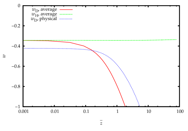
Another useful way of looking at the deviation of the distance–expansion rate relation from the FRW case is to define separate effective equations of state for the expansion rate and the distance [22, 21]. The effective expansion rate equation of state $w_{H}$ is defined as the equation of state of an extra energy density component that would give the expansion history $\bar{H}(z)$ in a spatially flat FRW model (with the same value of the dust density parameter $\Omega_{\mathrm{m0}}$ as in the backreaction model). From (3.19), (3.20) and (3.23) we have

$$w_{H} = \frac{2(1+z)\bar{H}\bar{H}^{\prime}-3\bar{H}^{2}}{3\bar{H}^{2}-8\pi G_{\mathrm{N}}\langle{\rho_{\mathrm{m}}}\rangle}=\frac{2q_{H}-1}{3-3\Omega_{\mathrm{m}}}\ .$$ (3.32)

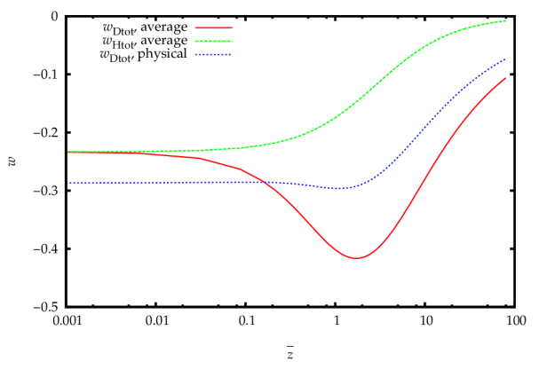
This definition is somewhat inconvenient, because $w_{H}$ diverges if at some moment the expansion rate is the same as in (and the acceleration is different from) the EdS model. In particular, this happens if the expansion rate decelerates first less and then more than in the EdS model, as could be expected if the expansion eventually accelerates [17, 18, 21]. (This also happens in some models with extra dimensions [89].) It is more informative to consider the total equation of state defined as

$$w_{H\mathrm{tot}} = (1+z)\frac{2\bar{H}^{\prime}}{3\bar{H}}-1=\frac{2q_{H}-1}{3}=\frac{\Omega_{\mathrm{m}}+4\Omega_{\mathcal{Q}}-1}{3}\ .$$ (3.33)

Correspondingly, the effective distance equation of state $w_{D}$ and the effective total distance equation of state $w_{D\mathrm{tot}}$ are defined to be those of the spatially flat FRW model with the same distance $D_{A}(z)$ (and $\Omega_{\mathrm{m0}}$) as the backreaction model, i.e. we replace $\bar{H}$ by $H_{\mathrm{fit}}$ and $\Omega_{\mathrm{m}}$ by $\Omega_{\mathrm{mfit}}(z)\equiv\Omega_{\mathrm{m0}}(1+z)^{3}(\bar{H}_{0}/H_{\mathrm{fit}}(z))^{2}$ in (3.32) and (3.33). We again use the redshift and the distance calculated from the average expansion rate with (3.25) and (3.26).

(a)

(b)

Figure 13: a) The effective equations of state $w_{H}$ and $w_{D}$. b) The effective equations of state $w_{H\mathrm{tot}}$ and $w_{D\mathrm{tot}}$.

We show the effective equations of state $w_{H}$ and $w_{D}$ in figure 13a, and $w_{H\mathrm{tot}}$ and $w_{D\mathrm{tot}}$ in figure 13b, again both for the distance and the redshift calculated from the average expansion rate using (3.25) and (3.26) and for the physical distance. The evolution of $w_{H}$ is close to that of a dust FRW model with an extra energy density component with equation of state close to $-\frac{1}{3}$. The equation of state $w_{D}$ is very different, but $w_{D\mathrm{tot}}$ gives a better picture of the distance. The behaviour of $w_{D\mathrm{tot}}$ is qualitatively similar for both distances, with a dip towards negative values. For the distance calculated from the average expansion rate, $w_{D\mathrm{tot}}$ goes below $-\frac{1}{3}$. Correspondingly, the deceleration parameter $q_{D}\equiv\frac{1}{2}(1+3w_{D\mathrm{tot}})$ shown in figure 6 is negative for a range of redshifts. However, the deceleration parameter that corresponds to the physical distance dips more moderately, and always remains positive. So the model has neither apparent acceleration nor average acceleration [11, 2]. Figure 13b demonstrates how the distance equation of state $q_{D}$ is biased towards more negative values (in general, towards $-1$) than $q_{H}$. As a result, average acceleration may not be needed to explain the observations [10, 11, 21]. This biasing can also alleviate tension between having a negative enough $q_{H}$ and a high enough $\bar{H}t$.

Such biasing is also present in the spatially curved FRW case. The inferred equation of state can be strongly affected if we try to determine the expansion rate of a FRW model assuming that it is spatially flat when spatial curvature is in fact non-zero [90]. For the distance calculated from the average expansion rate in the present model, the biasing can be understood in the same way, Even though the expansion rate is quite different from the spatially flat background FRW model, it is close to a negatively curved FRW model. This follows from the fact that $\Omega_{\mathcal{Q}}$ is small (i.e. $K$ is almost constant) at all times: then the integrability condition (3.22) implies that $\langle{{{}^{(3)}R}}\rangle\propto a^{-2}$, just as in the FRW case. Therefore, the difference between $w_{H}$ and $w_{D}$ can be understood in terms of the FRW distance–expansion rate relation (3.27): if we try to interpret the distance of a FRW model with $K<0$ in terms of a FRW model with $K=0$, the fitting model expansion rate will be larger than the real expansion rate to reproduce the effect of the $\sinh$ term. However, this is not the case for the physical distance: the relation between the average expansion rate and the physical distance cannot be understood simply in terms of a FRW spatial curvature. This is a general feature: if backreaction is significant, its effect cannot be encapsulated in a “global average FRW model” that would simultaneously account for both the expansion rate and the distance. This is expected to be the case even for the distance calculated from the average expansion rate, if the expansion first has extra deceleration and then accelerates [17, 18, 21]. Such behaviour could be reproduced by having regions with $E<0$ in the holes.

4 Discussion

Integral formulation and series formulation.

The reasoning behind relations (3.25) and (3.26) between the average expansion rate and redshift and distance is that if we integrate the light propagation equations, deviations around the average cancel because of statistical homogeneity and isotropy [22, 23]. Our results validate some aspects of this idea. In particular, the average expansion rate gives a good description of the redshift, though we have found that the contribution of the shear is important, in contrast to the arguments of [22, 23]. If we neglect jumps in the Sachs equations due to the surface layers, the angular diameter distance for $z\lesssim 1$ is also accurately calculable from the average expansion rate. The average expansion rate was also found to give a good description in [24], where the prescription was used that the time that light propagates in a given different region is proportional to the volume of the region, instead of considering light propagation in a complete spacetime that is a solution of the Einstein equation.

In contrast to the integral formulation (3.26) used in the present work and in [24], the redshift and the distance have also been considered in terms of a series expansion [91, 92, 93], which seems to give different results. In particular, it has been suggested that the distance can be quite different from the FRW case even when the average expansion rate is close to FRW [93]. The series formulation also suggests large angular variation in the distance. In [24] (see also [94]), the series formulation was found to disagree with the null geodesic calculation, unlike the integral formulation.

One issue with the series expansion is that the redshift along a null geodesic is in general not monotonic, so the distance cannot be written as a function of the redshift [22]. But even in models in which this is not the case, a series expansion can be misleading. If we approximate a function $f(z)$ between $z=0$ and $z=z_{1}$ with a Taylor series with terms up to $z^{n}$, the remainder term is bounded by $f^{(n+1)}_{\mathrm{max}}z^{n+1}/(n+1)!$, where $f^{(n+1)}_{\mathrm{max}}$ is the maximum value of $\mathrm{d}^{n+1}f/\mathrm{d}z^{\mathrm{n+1}}$ between $0$ and $z_{1}$. Therefore, the series expansion is inaccurate for rapidly varying functions. For non-analytic functions the series does not approximate the function even for small $z$, even if it converges. For example, consider the expansion rate as a function of redshift for an observer located on the edge of a stabilised region such as a galaxy. The expansion rate and its derivatives vanish at the location of the observer. As the function is not analytic, the Taylor series does not describe it. More realistically, it could be said that physically the local expansion rate is never exactly zero, and all functions can be approximated by Taylor series. In this case the problem is that the derivatives are large. The expansion rate changes rapidly by a factor of unity between a galaxy and an unbound region, and other quantities change even faster: the energy density varies by orders of magnitude over distances which are tiny on cosmological scales. In the models considered in [24] and in the present paper, variations are not so drastic, but there are nevertheless strong variations on scales that are small compared to the cosmological scale (in our case the density varies by about a factor of 40 between the most underdense and dense regions in a hole at the present time).

In the integral formulation, such rapid variations are not important because they cancel out, leaving only the average contribution. Averages of course depend on the hypersurface on which they are taken, and the relevant one for the line of sight integral is the hypersurface of statistical homogeneity and isotropy [18, 29, 22, 25, 23, 95, 96]. In the present case, this is the same as the hypersurface of constant proper time of the observers.

Usefulness of the average expansion rate.

It is perhaps surprising that the distance and the redshift calculated from the average expansion rate give such a good description of the physical distance (neglecting the jumps due to the surface layers) and redshift. After all, the average of the expansion rate is taken on the three-dimensional hypersurface of constant proper time, whereas cancellations in the deviations in the expansion rate along the null geodesic happen in one dimension. (It has even been questioned whether the average expansion rate has any physical relevance at all [26].) However, in Euclidean space with statistically homogeneous and isotropic (and static or slowly evolving) matter distribution, one-dimensional averages converge to three-dimensional averages, though this may require distances much longer than the homogeneity scale if the distribution is strongly clumped. (In the case of curved spacetime, the measures are different for a line integral and a volume integral, so the outcome is less clear.) For example, in the Millennium simulation, the matter distribution is very filamentary, and the one-dimensional average density seen by a typical light ray is about 20% smaller than the three-dimensional average even for distances of 1.5 Gpc [97, 36]. However, deviation of the distance from the background value is much smaller, less than 1% (see also [37]). Presumably this is related to the fact that the distance depends on the density via a double integral.

In the limit where the matter distribution consists of pointlike particles and the probability of a light ray crossing any matter vanishes, one could expect that the average expansion rate doesn’t give a useful description at all. However, the average expansion rate has been found to give a useful description also in the discrete models studied in [45, 46]. (Though one might worry that the geometrical optics approximation could break down [23].) In our model, the holes occupy a large fraction of space, so a light ray quickly samples a representative distribution of the expansion rate: a typical light ray spends approximately 50% of the travel time inside the holes.

It is sometimes claimed that light propagation in a clumpy universe is on average identical to the FRW situation simply because of flux conservation [98]. However, the proof presented in [98] assumes that the angular element is given by the FRW metric, which is the question to be investigated [99], and the LTB model has been used to provide an exact counterexample [100] (see also [101]). It has also been argued that the distance is close to FRW as long as light travels through compensated over- and underdensities, and the time spent by a light ray in a given region is much smaller than the timescale for the evolution of the gravitational potential of the region [43]. (This argument is tied to perturbation theory, as the gravitational potential is a perturbative concept.) However, our results, and those of [24], support the importance of the average expansion rate, not only the average density as in the Dyer-Roeder approximation [22, 23] (see also [24, 37, 36, 102]). It is the integrated effect over all regions that is relevant, not the time spent by the light in a given region. However, in order for the average expansion rate to give a good description, it is necessary that the distribution of structures does not change significantly during the time that it takes for a light ray to travel a spatial distance equal to the homogeneity scale.

Relation to Newtonian gravity.

In the spherically symmetric subcase, the result that backreaction is small is related to the fact that in Newtonian gravity, the average expansion rate of a spherical system is identical to the FRW case [82]. This result is well known under the name of spherical collapse model. It is sometimes claimed that the result would extend to general relativity (at times this is even ascribed to Birkhoff’s theorem; see section 2.5 of [2]). While this is not true in general, the spatially flat LTB model with $E=0$ is close to Newtonian gravity [59]. The structure of the general quasispherical Szekeres model is similar to that of the LTB model, as the metric depends on time only via $R(t,r)$, and for small, long-lived regular holes $E$ is small. From the geometrical point of view, the appearance of general relativistic degrees of freedom in the Szekeres model is constrained by the fact that the magnetic part of the Weyl tensor is zero. This is always true in Newtonian theory, but in general relativity dust models with vanishing magnetic Weyl tensor are a very limited class of solutions [61, 103, 104, 105, 106, 107, 25, 108]. It is conjectured that the Szekeres model is the only such inhomogeneous and irrotational solution [109] (a proof was claimed in [110]); whether the class of such solutions with rotation is non-empty is not known. The magnetic part of the Weyl tensor is non-zero in realistic solutions: for example, it is essential in gravitational collapse [104]. Its importance for the backreaction of realistic structures is not clear.

5 Conclusion

Summary and outlook.

We have proven that the average expansion rate in a Swiss Cheese dust model with Szekeres holes is close to the FRW model if the holes are small and long-lived, there are no singularities, the center of the hole is regular and the metric function $R$ is monotonic in the coordinate radius. By violating the last assumption, we have then built the first exact statistically homogeneous and isotropic solution in which inhomogeneity has a significant effect on the average expansion rate, i.e. backreaction is large. The expansion rate is close to the FRW case at early times, but increases relative to the background at late times. However, in the model, violating the monotonicity of $R$ requires surface layers.

We have studied the relation of the average expansion rate to the angular diameter distance and the redshift. The surface layers lead to large jumps in the area expansion rate of light bundles and sharp turning of light rays. We therefore consider a modified version of the distance in which we neglect the jumps due to the surface layers. For the redshift, we consider both the case when the light rays turn sharply as well as a modification in which we take them to follow straight paths as defined by the background metric. We find that the modified angular diameter distance is significantly different from the background, but it is fairly well described by the distance calculated from the average expansion rate up to redshifts of order unity, though not for larger redshifts. The redshift also differs markedly from the background value, and it is well described by the average expansion rate, with statistical fluctuations of less than 10% for the unmodified rays, and less than 5% for the straight rays. In contrast to expectation, the expansion rate along the light ray is not the same as the spatial average, though the difference cancels with the contribution of shear along the light ray. This situation is the same both for unmodified and straight rays.

The results show the usefulness of the spatially averaged expansion rate in describing light propagation. However, as the unrealistic surface layers have a large effect on light propagation, it would be interesting to consider models without them. One simple and physically motivated way to extend the present study and bypass our Szekeres Swiss Cheese theorem without surface layers would be to resolve unphysical shell crossing and collapse singularities either by introducing pressure [111] or by applying some other prescription to include interactions that prevent singularities in real structure formation [73].

Another issue related to the surface layers is that although the local expansion rate, shear and density asymptotically approach FRW values at early times, this is not the case for the metric nor the spatial curvature. It would be interesting to construct exact solutions in which the metric is perturbatively close to FRW at early times, but backreaction is nevertheless large at late times.

References

- [1]
- [2] T. Buchert and S. Räsänen, Backreaction in late-time cosmology, Ann. Rev. Nucl. Part. Sci. 62 (2012) 57 [arXiv:1112.5335 [astro-ph.CO]]
- [3] M.F. Shirokov and I.Z. Fisher, Isotropic Space with Discrete Gravitational-Field Sources. On the Theory of a Nonhomogeneous Universe, Astronomicheskii Zhurnal 39 (1962) 899, Reprinted in Sov. Astron. J. 6 (1963) 699, Reprinted in Gen. Rel. Grav. 30 (1998) 1411
-
[4]
G.F.R. Ellis,
Relativistic cosmology: its nature, aims and problems, 1984
The invited papers of the 10th international conference on general relativity and gravitation
p. 215
G.F.R. Ellis and W. Stoeger, The ’fitting problem’ in cosmology, Class. Quant. Grav. 4 (1987) 1697 - [5] T. Buchert and J. Ehlers, Averaging inhomogeneous Newtonian cosmologies, Astron. & Astrophys. 320 (1997) 1 [arXiv:astro-ph/9510056]
- [6] T. Buchert, On average properties of inhomogeneous fluids in general relativity I: dust cosmologies, Gen. Rel. Grav. 32 (2000) 105 [arXiv:gr-qc/9906015]
- [7] T. Buchert, On average properties of inhomogeneous fluids in general relativity II: perfect fluid cosmologies, Gen. Rel. Grav. 33 (2001) 1381 [arXiv:gr-qc/0102049]
- [8] G.F.R. Ellis and T. Buchert, The universe seen at different scales, Phys. Lett. A347 (2005) 38 [arXiv:gr-qc/0506106]
- [9] T. Buchert, Dark Energy from Structure - A Status Report, Gen. Rel. Grav. 40 (2008) 467 [arXiv:0707.2153 [gr-qc]]
- [10] S. Räsänen, Backreaction as an alternative to dark energy and modified gravity [arXiv:1012.0784 [astro-ph.CO]]
- [11] S. Räsänen, Backreaction: directions of progress, Class. Quant. Grav. 28 (2011) 164008 [arXiv:1102.0408 [astro-ph.CO]]
- [12] T. Buchert, On average properties of inhomogeneous cosmologies, 2000, Proc. 9th JGRG conference, ed. Y. Eriguchi et al. , p. 306 [arXiv:gr-qc/0001056]
- [13] C. Wetterich, Can Structure Formation Influence the Cosmological Evolution?, Phys. Rev. D67 (2003) 043513 [arXiv:astro-ph/0111166]
- [14] D.J. Schwarz, Accelerated expansion without dark energy [arXiv:astro-ph/0209584]
[15]
S. Räsänen,
Dark energy from backreaction,
JCAP02(2004)003
[arXiv:astro-ph/0311257]
S. Räsänen, Backreaction of linear perturbations and dark energy [arXiv:astro-ph/0407317] - [16] E.W. Kolb, S. Matarrese, A. Notari and A. Riotto, The effect of inhomogeneities on the expansion rate of the universe, Phys. Rev. D71 (2005) 023524 [arXiv:hep-ph/0409038]
- [17] S. Räsänen, Cosmological acceleration from structure formation, Int. J. Mod. Phys. D15 (2006) 2141 [arXiv:astro-ph/0605632]
- [18] S. Räsänen, Accelerated expansion from structure formation, JCAP11(2006)003 [arXiv:astro-ph/0607626]
[19]
C.H. Chuang, J.A. Gu and W.Y. Hwang,
Inhomogeneity-Induced Cosmic Acceleration in a Dust Universe,
Class. Quant. Grav. 25 (2008) 175001
[arXiv:astro-ph/0512651]
A. Paranjape and T.P. Singh, The Possibility of Cosmic Acceleration via Spatial Averaging in Lemaître-Tolman-Bondi Models, Class. Quant. Grav. 23 (2006) 6955 [arXiv:astro-ph/0605195]
A. Paranjape, The Averaging Problem in Cosmology, Ph.D. thesis, Tata Institute of Fundamental Research, Mumbai, 2009 [arXiv:0906.3165 [astro-ph.CO]] - [20] T. Kai, H. Kozaki, K.-i. Nakao, Y. Nambu and C.M. Yoo, Can inhomogeneities accelerate the cosmic volume expansion?, Prog. Theor. Phys. 117 (2007) 229 [arXiv:gr-qc/0605120]
- [21] C. Boehm and S. Räsänen, Violation of the FRW consistency condition as a signature of backreaction [arXiv:1305.7139 [astro-ph.CO]]
- [22] S. Räsänen, Light propagation in statistically homogeneous and isotropic dust universes, JCAP02(2009)011 [arXiv:0812.2872 [astro-ph]]
- [23] S. Räsänen, Light propagation in statistically homogeneous and isotropic universes with general matter content, JCAP03(2010)018 [arXiv:0912.3370 [astro-ph.CO]]
- [24] P. Bull and T. Clifton, Local and non-local measures of acceleration in cosmology, Phys. Rev. D85 (2012) 103512 [arXiv:1203.4479 [astro-ph.CO]]
- [25] S. Räsänen, Light propagation and the average expansion rate in near-FRW universes, Phys. Rev. D85 (2012) 083528 [arXiv:1107.1176 [astro-ph.CO]]
[26]
S.R. Green and R.M. Wald,
A new framework for analyzing the effects of small scale inhomogeneities in cosmology,
Phys. Rev. D83 (2011) 084020
[arXiv:1011.4920 [gr-qc]]
S.R. Green and R.M. Wald, Examples of backreaction of small scale inhomogeneities in cosmology [arXiv:1304.2318 [gr-qc]] - [27] S.J. Szybka, K. Glod, M.J. Wyrebowski and A. Konieczny, Inhomogeneity effect in Wainwright-Marshman space-times [arXiv:1306.1783 [gr-qc]]
- [28] C. Rampf and G. Rigopoulos, Zel’dovich Approximation and General Relativity, Mon. Not. Roy. Astron. Soc. 430 (2013) L54 [arXiv:1210.5446 [astro-ph.CO]]
- [29] S. Räsänen, Evaluating backreaction with the peak model of structure formation, JCAP04(2008)026 [arXiv:0801.2692 [astro-ph]]
[30]
The effect of structure formation on the expansion of the universe,
Int. J. Mod. Phys. D17 (2008) 2543
[arXiv:0805.2670 [astro-ph]]
S. Räsänen, Structure formation as an alternative to dark energy and modified gravity, EAS Publications Series (2009) 36 63 [arXiv:0811.2364 [astro-ph]] -
[31]
R. Kantowski,
Corrections in the Luminosity-Redshift Relations of the Homogeneous Friedmann Models,
Astrophys. J. 155 (1969) 89
N. Sugiura, K.-i. Nakao, D. Ida, N. Sakai and H. Ishihara, How do nonlinear voids affect light propagation?, Prog. Theor. Phys. 103 (2000) 73 [arXiv:astro-ph/9912414]
N. Brouzakis, N. Tetradis and E. Tzavara, The Effect of Large-Scale Inhomogeneities on the Luminosity Distance JCAP02(2007)013 [arXiv:astro-ph/0612179]
T. Biswas and A. Notari, Swiss-Cheese Inhomogeneous Cosmology and the Dark Energy Problem, JCAP06(2008)021 [arXiv:astro-ph/0702555]
N. Brouzakis, N. Tetradis N and E. Tzavara, Light Propagation and Large-Scale Inhomogeneities, JCAP04(2008)008 [arXiv:astro-ph/0703586]
V. Marra, E.W. Kolb, S. Matarrese and A. Riotto, On cosmological observables in a swiss-cheese universe, Phys. Rev. D76 (2007) 123004 [0708.3622 [astro-ph]]
V. Marra, E. W. Kolb and S. Matarrese, Light-cone averages in a swiss-cheese Universe, Phys. Rev. D77 (2008) 023003 [arXiv:0710.5505 [astro-ph]]
N. Brouzakis and N. Tetradis, Analytical Estimate of the Effect of Spherical Inhomogeneities on Luminosity Distance and Redshift, Phys. Lett. B665 (2008) 344 [arXiv:0802.0859 [astro-ph]]
V. Marra, On cosmological observables in a swiss-cheese universe (Conference proceeding), Proc. of 43rd Rencontres de Moriond, [arXiv:0805.4233 [astro-ph]]
R.A. Vanderveld, É.É. Flanagan and I. Wasserman, Luminosity distance in ’Swiss cheese’ cosmology with randomized voids: I. Single void size, Phys. Rev. D78 (2008) 083511 [arXiv:0808.1080 [astro-ph]]
T. Clifton and J. Zuntz, Hubble Diagram Dispersion From Large-Scale Structure, Mon. Not. Roy. Astron. Soc. 400 (2009) 2185 [arXiv:0902.0726 [astro-ph.CO]]
W. Valkenburg, Swiss Cheese and a Cheesy CMB JCAP06(2009)010 [arXiv:0902.4698 [astro-ph.CO]]
V. Kostov, Average luminosity distance in inhomogeneous universes, JCAP04(2010)001 [arXiv:0910.2611 [astro-ph.CO]]
E.E. Flanagan, N. Kumar, I. Wasserman and R.A. Vanderveld, Luminosity distance in Swiss cheese cosmology with randomized voids. II. Magnification probability distributions, Phys. Rev. D85 (2012) 023510 [arXiv:1109.1873 [gr-qc]]
E.E. Flanagan, N. Kumar and I. Wasserman, Luminosity distance in Swiss cheese cosmology with randomized voids and galaxy halos, arXiv:1207.3711 [astro-ph.CO]
P. Fleury, Hélèn. Dupuy and J.-P. Uzan, Interpretation of the Hubble diagram in a non-homogeneous universe [arXiv:1302.5308 [astro-ph.CO]] -
[32]
K. Bolejko,
The Szekeres Swiss Cheese model and the CMB observations,
Gen. Rel. Grav. 41 (2009) 1737
[arXiv:0804.1846 [astro-ph]]
K. Bolejko and M. -N. Célérier, Szekeres Swiss-Cheese model and supernova observations, Phys. Rev. D82 (2010) 103510 [arXiv:1005.2584 [astro-ph.CO]] - [33] K. Bolejko, Weak lensing and the Dyer-Roeder approximation, Mon. Not. Roy. Astron. Soc. 412 (2011) 1937 [arXiv:1011.3876 [astro-ph.CO]]
- [34] S.J. Szybka, On light propagation in Swiss-Cheese cosmologies, Phys. Rev. D64 (2011) 044011 [arXiv:1012.5239 [astro-ph.CO]]
- [35] K. Bolejko, The effect of inhomogeneities on the distance to the last scattering surface and the accuracy of the CMB analysis JCAP02(2011)025 [arXiv:1101.3338 [astro-ph.CO]]
- [36] C. Clarkson, G. Ellis, A. Faltenbacher, R. Maartens, O. Umeh and J.P. Uzan, (Mis-)interpreting supernovae observations in a lumpy universe, Mon. Not. Roy. Astron. Soc. 426 (2012) 1121 [arXiv:1109.2484 [astro-ph.CO]]
- [37] K. Bolejko and P.G. Ferreira, Ricci focusing, shearing, and the expansion rate in an almost homogeneous Universe, JCAP05(2012)003 [arXiv:1204.0909 [astro-ph.CO]]
- [38] S. Räsänen, On the relation between the isotropy of the CMB and the geometry of the universe, Phys. Rev. D79 (2009) 123522 [arXiv:0903.3013 [astro-ph.CO]]
- [39] K. Enqvist and T. Mattsson, The effect of inhomogeneous expansion on the supernova observations, JCAP02(2007)019 [arXiv:astro-ph/0609120]
- [40] K. Bolejko and L. Andersson, Apparent and average acceleration of the Universe, JCAP10(2008)003 [arXiv:0807.3577 [astro-ph]]
- [41] E.W. Kolb and C.R. Lamb, Light-cone observations and cosmological models: implications for inhomogeneous models mimicking dark energy [arXiv:0911.3852 [astro-ph.CO]]
- [42] N. Meures and M. Bruni, Redshift and distances in a CDM cosmology with non-linear inhomogeneities, Mon. Not. Roy. Astron. Soc. 419 (2012) 1937 [arXiv:1107.4433 [astro-ph.CO]]
- [43] E. Di Dio, M. Vonlanthen and R. Durrer, Back Reaction from Walls, JCAP02(2012)036 [arXiv:1111.5764 [astro-ph.CO]]
- [44] C. Hellaby, A new type of exact arbitrarily inhomogeneous cosmology: Evolution of deceleration in the flat homogeneous-on-average case, JCAP01(2012)043 [arXiv:1203.3652 [gr-qc]]
[45]
T. Clifton and P.G. Ferreira,
Archipelagian Cosmology: Dynamics and Observables in a Universe with Discretized Matter Content,
Phys. Rev. D80 (2009) 103503 (errata: Phys. Rev. D84 (2011) 109902(E))
[arXiv:0907.4109 [astro-ph.CO]]
T. Clifton and P.G. Ferreira, Errors in Estimating due to the Fluid Approximation, JCAP10(2009)26 [arXiv:0908.4488 [astro-ph.CO]]
T. Clifton, P.G. Ferreira and K. O’Donnell, An Improved Treatment of Optics in the Lindquist-Wheeler Models, Phys. Rev. D85 (2012) 023502 [arXiv:1110.3191 [astro-ph.CO]] -
[46]
J.P. Bruneton and J. Larena,
Dynamics of a lattice Universe: The dust approximation in cosmology,
Class. Quant. Grav. 29 (2012) 155001
[arXiv:1204.3433 [gr-qc]]
J.P. Bruneton and J. Larena, Observables in a lattice Universe, Class. Quant. Grav. 30 (2013) 025002 [arXiv:1208.1411 [gr-qc]]
J. Larena, The fitting problem in a lattice Universe [arXiv:1210.2161 [astro-ph.CO]]
J.-P. Bruneton, MG13 Proceedings: A lattice Universe as a toy-model for inhomogeneous cosmology [arXiv:1303.0174 [gr-qc]] -
[47]
C.-M. Yoo, H. Abe, K.-i. Nakao and Y. Takamori,
Black Hole Universe: Construction and Analysis of Initial Data,
Phys. Rev. D86 (2012) 044027
[arXiv:1204.2411 [gr-qc]]
E. Bentivegna and M. Korzynski, Evolution of a periodic eight-black-hole lattice in numerical relativity, Class. Quant. Grav. 29 (2012) 165007 [arXiv:1204.3568 [gr-qc]]
E. Bentivegna, Black-hole lattices [arXiv:1307.7673 [gr-qc]] - [48] T. Clifton, K. Rosquist and R. Tavakol, An Exact quantification of backreaction in relativistic cosmology, Phys. Rev. D86 (2012) 043506 [arXiv:1203.6478 [gr-qc]]
- [49] C. Bonvin, R. Durrer and M.A. Gasparini, Fluctuations of the luminosity distance, Phys. Rev. D73 (2006) 023523, erratum Phys. Rev. D85 (2012) 029901 [arXiv:astro-ph/0511183]
- [50] I. Ben-Dayan, M. Gasperini, G. Marozzi, F. Nugier and G. Veneziano, Backreaction on the luminosity-redshift relation from gauge invariant light-cone averaging, JCAP04(2012)036 [arXiv:1202.1247 [astro-ph.CO]]
[51]
I. Ben-Dayan, M. Gasperini, G. Marozzi, F. Nugier and G. Veneziano,
Do stochastic inhomogeneities affect dark-energy precision measurements?,
Phys. Rev. Lett. 110 (2013) 021301
[arXiv:1207.1286 [astro-ph.CO]]
I. Ben-Dayan, M. Gasperini, G. Marozzi, F. Nugier and G. Veneziano, Average and dispersion of the luminosity-redshift relation in the concordance model, JCAP06(2013)002 [arXiv:1302.0740 [astro-ph.CO]] - [52] V. Marra and A. Notari, Observational constraints on inhomogeneous cosmological models without dark energy, Class. Quant. Grav. 28 (2011) 164004 [arXiv:1102.1015 [astro-ph.CO]]
[53]
P. Szekeres,
A class of inhomogeneous cosmological models,
Commun. Math. Phys. 41 (1975) 55
C. Hellaby and A. Krasinski, You can’t get through Szekeres wormholes: Or, regularity, topology and causality in quasispherical Szekeres models, Phys. Rev. D66 (2002) 084011 [arXiv:gr-qc/0206052]
C. Hellaby and A. Krasinski, Physical and geometrical interpretation of the Szekeres models, Phys. Rev. D77 (2008) 023529 [arXiv:0710.2171 [gr-qc]]
A. Krasinski, Geometry and topology of the quasi-plane Szekeres model, Phys. Rev. D78 (2008) 064038 Erratum Phys. Rev. D85 (2012) 069903 [arXiv:0805.0529 [gr-qc]] - [54] J. Plebanski and A. Krasiński, An Introduction to General Relativity and Cosmology, 2006 Cambridge University Press, Cambridge
- [55] A.G. Lemaître, The Expanding Universe, Ann. Soc. Sci Bruxelles A53 (1933) 51 (in French) Reprinted in Gen. Rel. Grav. 29 (1997) 641
- [56] R.C. Tolman, Effect of Inhomogeneity on Cosmological Models, Proc. Nat. Acad. Sci. USA 20 (1934) 169 Reprinted in Gen. Rel. Grav. 29 (1997) 935
- [57] H. Bondi, Spherically symmetrical models in general relativity, Mon. Not. Roy. Astron. Soc. 107 (1947) 410
- [58] C. Hellaby and K. Lake, Shell crossings and the Tolman model, Astrophys. J. 290 (1985) 381 Erratum in Astrophys. J. 300 (1986) 461
- [59] P. Szekeres and A. Lun, What is a shell crossing singularity?, J. Austral. Math. Soc. B41 (1999) 167
- [60] J. Ehlers, Contributions to the relativistic mechanics of continuous media, Abh. Akad. Wiss. Lit. Mainz. Nat. Kl. 11 (1961) 792 (in German) Reprinted in Gen. Rel. Grav. 25 (1993) 1225
- [61] G.F.R. Ellis, Relativistic Cosmology, 1971, General Relativity and Cosmology, ed. R.K. Sachs, Academic Press Inc., London, p. 104, Reprinted in Gen. Rel. Grav. 41 (2009) 581
- [62] G.F.R. Ellis and H. van Elst, Cosmological models (Cargèse lectures 1998), NATO Adv. Study Inst. Ser. C. Math. Phys. Sci. 541 (1999) 1 [arXiv:gr-qc/9812046]
- [63] C.G. Tsagas, A. Challinor and R. Maartens, Relativistic cosmology and large-scale structure, Phys. Rept. 465 (2008) 61 [arXiv:0705.4397 [astro-ph]]
- [64] S. Magni, Backreaction and the Covariant Formalism of General Relativity, Master’s thesis, University of Pavia, 2011 [arXiv:1202.0430 [gr-qc]]
[65]
G. Darmois,
Mémorial des sciences mathématiques,
fascicule 25 (1927) 1, p. 28
W. Israel, Singular hypersurfaces and thin shells in general relativity, Nuovo Cim. B44 (1966) 1, Erratum Nuovo Cim. B48 (1967) 463
W.B. Bonnor and P.A. Vickers, Junction conditions in general relativity, Gen. Rel. Grav. 13 (1981) 29
M. Carrera and D. Giulini, On the influence of global cosmological expansion on the dynamics and kinematics of local systems, Rev. Mod. Phys. 82 (2010) 169 [arXiv:0810.2712 [gr-qc]] - [66] D.R. Matravers and N.P. Humphreys, Matching spherical dust solutions to construct cosmological models, Gen. Rel. Grav. 33 (2001) 531 [arXiv:gr-qc/0009057]
- [67] M. Mars, F.C. Mena and R.Vera, Review on exact and perturbative deformations of the Einstein-Straus model: uniqueness and rigidity results [arXiv:1307.4371 [gr-qc]]
- [68] W.B. Bonnor, Closed Tolman models of the universe, Class. Quant. Grav. 2 (1985) 781
- [69] N.P. Humphreys, R. Maartens and D.R. Matravers, newblock Regular spherical dust space-times, Gen. Rel. Grav. 44 (2012) 3197 [arXiv:gr-qc/9804023]
- [70] T. Shiromizu, K. -i. Maeda and M. Sasaki, The Einstein equation on the 3-brane world, Phys. Rev. D62 (2000) 024012 [arXiv:gr-qc/9910076]
- [71] R.A. Sussman, Back-reaction and effective acceleration in generic LTB dust models, Class. Quant. Grav. 28 (2011) 235002 [arXiv:1102.2663 [gr-qc]]
- [72] K. Bolejko, Volume averaging in the quasispherical Szekeres model, Gen. Rel. Grav. 41 (2009) 1585 [arXiv:0808.0376 [astro-ph]]
[73]
S. Engineer, N. Kanekar and T. Padmanabhan,
Nonlinear density evolution from an improved spherical collapse model,
Mon. Not. Roy. Astron. Soc. 314 (2000) 279
[arXiv:astro-ph/9812452]
Buchert T and Domínguez A, Adhesive Gravitational Clustering, Astron. & Astrophys. 438 (2005) 443 [arXiv:astro-ph/0502318]
D.J. Shaw and D.F. Mota, An Improved Semi-Analytical Spherical Collapse Model for Non-linear Density Evolution, Astrophys. J. Suppl. 174 (2008) 277 [arXiv:0708.0868 [astro-ph]] - [74] C. Cederbaum, The Newtonian Limit of Geometrostatics, Ph.D. thesis, Freie Universit’́at Berlin, 2011 [arXiv:1201.5433 [gr-qc]]
- [75] J. Silk, Large-scale inhomogeneity of the Universe - Spherically symmetric models, Astron. & Astrophys. 59 (1977) 53
- [76] P.M. Sutter, G. Lavaux, B.D. Wandelt and D.H. Weinberg, A public void catalog from the SDSS DR7 Galaxy Redshift Surveys based on the watershed transform, Astrophys. J. 761 (2012) 44 [arXiv:1207.2524 [astro-ph.CO]]
[77]
M.A. Aragon-Calvo, R. van de Weygaert and B.J.T. Jones,
Multiscale Phenomenology of the Cosmic Web,
Mon. Not. Roy. Astron. Soc. 408 (2010) 2163
[arXiv:1007.0742 [astro-ph.CO]]
M. Cautun, R. van de Weygaert and B.J.T. Jones, NEXUS: Tracing the Cosmic Web Connection, Mon. Not. Roy. Astron. Soc. 429 (2013) 1286 [arXiv:1209.2043 [astro-ph.CO]] - [78] P. Schneider, J. Ehlers and E.E. Falco, Gravitational Lenses, 1992 Springer-Verlag, New York
- [79] M. Sasaki, Cosmological Gravitational Lens Equation: Its Validity And Limitation, Prog. Theor. Phys. 90 (1993) 753
- [80] A.G. Riess et al., A 3% Solution: Determination of the Hubble Constant with the Hubble Space Telescope and Wide Field Camera 3, Astrophys. J. 730 (2011) 119 [arXiv:1103.2976 [astro-ph.CO]]
- [81] V. Marra, M. Pääkkönen and W. Valkenburg, Bias on w from large-scale structure, Mon. Not. Roy. Astron. Soc. 431 (2013) 1891 [arXiv:1203.2180 [astro-ph.CO]]
- [82] T. Buchert, M. Kerscher and C. Sicka, Backreaction of inhomogeneities on the expansion: the evolution of cosmological parameters, Phys. Rev. D62 (2000) 043525 [arXiv:astro-ph/9912347]
- [83] S. Räsänen, Constraints on backreaction in dust universes, Class. Quant. Grav. 23 (2006) 1823 [arXiv:astro-ph/0504005]
- [84] I.M.H. Etherington, On the definition of distance in general relativity, Philosophical Magazine 15 (1933) 761 Reprinted in Gen. Rel. Grav. 39 (2007) 1055
- [85] C. Clarkson, B.A. Bassett and T.C. Lu, A general test of the Copernican Principle, Phys. Rev. Lett. 101 (2008) 011301 [arXiv:0712.3457 [astro-ph]]
- [86] A. Shafieloo and C. Clarkson, Model independent tests of the standard cosmological model, Phys. Rev. D81 (2010) 083537 [arXiv:0911.4858 [astro-ph.CO]]
- [87] E. Mörtsell and J. Jönsson, A model independent measure of the large scale curvature of the Universe [arXiv:1102.4485 [astro-ph.CO]]
- [88] S. February, J. Larena, M. Smith and C. Clarkson, Rendering Dark Energy Void, Mon. Not. Roy. Astron. Soc. 405 (2010) 2231 [arXiv:0909.1479 [astro-ph.CO]]
[89]
F. Ferrer and S. Räsänen,
Dark energy and decompactification in string gas cosmology,
JHEP02(2006)016
[arXiv:hep-th/0509225]
F. Ferrer, T. Multamäki and S. Räsänen, Fitting oscillating string gas cosmology to supernova data, JHEP04(2009)006 [arXiv:0812.4182 [hep-th]]
F. Ferrer, Cosmological acceleration from a gas of strings, Nucl. Phys. Proc. Suppl. 194 (2009) 218 [arXiv:0907.1342 [hep-th]] - [90] C. Clarkson, M. Cortês M and B.A.Bassett, Dynamical dark energy or simply cosmic curvature?, JCAP08(2007)011 [arXiv:astro-ph/0702670]
- [91] J. Kristian and R.H. Sachs, Observations In Cosmology, Astrophys. J. 143 (1966) 379
- [92] C.A. Clarkson, On the Observational Characteristics of Inhomogeneous Cosmologies: Undermining the Cosmological Principle Ph.D. thesis, University of Glasgow, 1999 [arXiv:astro-ph/0008089]
- [93] C. Clarkson and O. Umeh, Is backreaction really small within concordance cosmology?, Class. Quant. Grav. 28 (2011) 164010 [arXiv:1105.1886 [astro-ph.CO]]
- [94] T. Clifton, ‘Back-Reaction in Relativistic Cosmology, Int. J. Mod. Phys. D22 (2013) 133004 [arXiv:1302.6717 [gr-qc]]
[95]
G. Geshnizjani and R. Brandenberger,
Back Reaction And Local Cosmological Expansion Rate,
Phys. Rev. D66 (2002) 123507
[arXiv:gr-qc/0204074]
G. Geshnizjani and R. Brandenberger, Back Reaction Of Perturbations In Two Scalar Field Inflationary Models, JCAP04(2005)006 [arXiv:hep-th/0310265] - [96] S. Räsänen, Backreaction in the Lemaître-Tolman-Bondi model, JCAP11(2004)010 [arXiv:gr-qc/0408097]
- [97] K. Bolejko, private communication.
- [98] S. Weinberg, Apparent Luminosities In A Locally Inhomogeneous Universe, Astrophys. J. 208 (1976) L1
- [99] G.F.R. Ellis, B.A. Bassett and P.K.S. Dunsby, Lensing and caustic effects on cosmological distances, Class. Quant. Grav. 15 (1998) 2345 [arXiv:gr-qc/9801092]
- [100] N. Mustapha, B.A. Bassett, C. Hellaby and G.F.R. Ellis, Shrinking II – The Distortion of the Area Distance-Redshift Relation in Inhomogeneous Isotropic Universes, Class. Quant. Grav. 15 (1998) 2363 [arXiv:gr-qc/9708043]
- [101] G.F.R. Ellis and D.M. Solomons, Caustics of compensated spherical lens models, Class. Quant. Grav. 15 (1998) 2381 [arXiv:gr-qc/9802005]
- [102] J. Ehlers and P. Schneider, Self-consistent probabilities for gravitational lensing in inhomogeneous universes, Astron. & Astrophys. 168 (1986) 57
- [103] G.F.R. Ellis and P.K.S. Dunsby, Newtonian evolution of the Weyl tensor, Astrophys. J. 479 (1997) 97 [arXiv:astro-ph/9410001]
- [104] L. Kofman and D. Pogosyan, Dynamics of gravitational instability is nonlocal, Astrophys. J. 442 (1995) 30
- [105] S. Matarrese and D. Terranova, Post-Newtonian Cosmological Dynamics in Lagrangian Coordinates, Mon. Not. Roy. Astron. Soc. 283 (1996) 400 [arXiv:astro-ph/9511093]
- [106] J. Ehlers and T. Buchert, On the Newtonian Limit of the Weyl Tensor, Gen. Rel. Grav. 41 (2009) 2153 [arXiv:0907.2645 [gr-qc]]
- [107] S. Räsänen, Applicability of the linearly perturbed FRW metric and Newtonian cosmology, Phys. Rev. D81 (2010) 103512 [arXiv:1002.4779 [astro-ph.CO]]
- [108] U. Bertello, Cosmology in the Newtonian limit, Master’s thesis, University of Helsinki, 2012 [arXiv:1203.5596 [astro-ph.CO]]
[109]
H. van Elst, C. Uggla, W.M. Lesame, G.F.R. Ellis and R. Maartens,
Integrability of Irrotational Silent Cosmological Models,
Class. Quant. Grav. 14 (1997) 1151
[arXiv:gr-qc/9611002]
C.F. Sopuerta, New study of silent universes, Phys. Rev. D55 (1997) 5936 - [110] P.S. Apostolopoulos and J. Carot, Uniqueness of Petrov type D spatially inhomogeneous irrotational silent models, Int. J. Mod. Phys. D22 (2007) 1983 [arXiv:gr-qc/0605130]
- [111] K. Bolejko and P. Lasky, Pressure gradients, shell crossing singularities and acoustic oscillations - application to inhomogeneous cosmological models, Mon. Not. Roy. Astron. Soc. 391 (2008) L59 [arXiv:0809.0334 [astro-ph]]