External Potential Flow Around Multiple Aerofoils

^aDepartment of Mathematics, Faculty of Science, King Khalid University,

P. O. Box 9004, Abha 61413, Saudi Arabia.

E-mail: mms_nasser@hotmail.com

^bDepartment of Mathematical Sciences, Faculty of Science,

Universiti Teknologi Malaysia, 81310 UTM Johor Bahru, Johor, Malaysia

E-mail: mi@mel.fs.utm.my

1 Introduction

In this chapter, we consider the two dimensional, steady-state, irrotational flow around multiple aerofoils of general shape. We assume that the fluid is incompressible and free from viscosity and the boundaries of the aerofoils are stationary and impervious. The problem will be solved using a fast boundary integral method based on the boundary integral equation with the generalized Neumann kernel presented in [9]. The integral equation will be solved using the fast method presented in [15] which is based on discretizing the integral equation using the Nyström method with the trapezoidal rule then solving the obtained linear system by the generalized minimal residual (GMRES) method [16]. The GMRES method will converge significantly faster since the eigenvalues of the coefficient matrix of the linear system are clustered around $1$ (see [12, 13, 14]). Each iteration of the GMRES method requires a matrix-vector product which can be computed using the Fast Multipole Method (FMM) in $O(mn)$ operations where $m$ is the number of aerofoils and $n$ is the number of nodes in the discretization of each aerofoil’s boundary. Computing the right-hand side of the integral equation requires applying the FFT for each of the $m$ aerofoils which requires $O(mn\ln n)$ operations. Thus, the complexity of the presented method is $O(mn\ln n)$.

Three numerical examples will be presented. The numerical results illustrate that the present method has the ability to handle regions with very high connectivity and complex geometry.

2 Notations and auxiliary material

We consider an unbounded multiply connected regions $G$ in the extended complex plane $\overline{\mathbb{C}}$ exterior to $m\geq 1$ simply connected regions $G_{j}$, $j=1,2,\ldots,m$. We assume that the region $G$ is filled with an irrotational incompressible fluid flow and the bounded regions $G_{j}$, $j=1,2,\dots,m$, represents $m$ aerofoils or obstacles in the flow path. We assume that the boundaries $\Gamma_{j}:=\partial G_{j}$ of the aerofoils are smooth closed Jordan curves. The orientation of the whole boundary $\Gamma:=\partial G=\cup_{j=1}^{m}\Gamma_{j}$ is such that $G$ is always on the left of $\Gamma$, i.e., the curves $\Gamma_{1},\dots,\Gamma_{m}$ always have clockwise orientations (see Fig. 1).

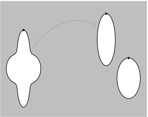
$\Gamma_{2}$
                                                                                   $G_{2}$                               $\Gamma_{m}$
                                                                                                  $\Gamma_{1}$                               $G_{m}$                                                                                                   $G_{1}$                                                              $G$

Figure 1: An unbounded multiply connected region $G$ of connectivity $m$.

The curve $\Gamma_{j}$ is parametrized by a $2\pi$-periodic twice continuously differentiable complex function $\eta_{j}(t)$ with non-vanishing first derivative

$$\dot{\eta}_{j}(t)=d\eta_{j}(t)/dt\neq 0,\quad t\in J_{j}:=[0,2\pi],\quad j=1,2,\ldots,m.$$ (1)

We define the total parameter domain $J$ as the disjoint union of the intervals $J_{j}$. Hence, a parametrization of the whole boundary $\Gamma$ is defined as the complex function $\eta$ defined on $J$ by

$$\eta(t):=\left\{\begin{array}[]{l@{\hspace{1cm}}l}\eta_{1}(t),\hfil\hskip 28.45274pt&t\in J_{1},\\ \vdots\hfil\hskip 28.45274pt&\\ \eta_{m}(t),\hfil\hskip 28.45274pt&t\in J_{m}.\\ \end{array}\right.$$ (2)

The definition of the function $\eta(t)$ in (2) means that for a given real number $\hat{t}\in[0,2\pi]$, to evaluate $\eta(\hat{t})$, we should know in advance the interval $J_{j}$ to which $\hat{t}$ belongs, i.e., we should know the boundary $\Gamma_{j}$ contains the point $\eta(\hat{t})$, then we compute $\eta(\hat{t})=\eta_{j}(\hat{t})$.

The real kernel $N$ defined by

$$N(s,t)=\frac{1}{\pi}\mathop{\mathrm{Im}}\left(\frac{\dot{\eta}(t)}{\eta(t)-\eta(s)}\right).$$ (3)

is known as the Neumann kernel. It is special case of the generalized Neumann kernel with $A=1$. The kernel $N$ is continuous with

$$N(t,t)=\frac{1}{2\pi}\mathop{\mathrm{Im}}\frac{\ddot{\eta}(t)}{\dot{\eta}(t)}.$$ (4)

The real kernel $M$ defined by

$$M(s,t)=\frac{1}{\pi}\mathop{\mathrm{Re}}\left(\frac{\dot{\eta}(t)}{\eta(t)-\eta(s)}\right),$$ (5)

has a cotangent singularity type. When $s,t\in J_{j}$ are in the same parameter interval $J_{j}$, then

$$M(s,t)=-\frac{1}{2\pi}\cot\frac{s-t}{2}+M_{1}(s,t)$$ (6)

with a continuous kernel $M_{1}$ which takes on the diagonal the values

$$M_{1}(t,t)=\frac{1}{2\pi}\mathop{\mathrm{Re}}\frac{\ddot{\eta}(t)}{\dot{\eta}(t)}.$$ (7)

See [3, 5, 8, 14, 17, 18] for more details.

We define the Fredholm integral operator with the kernel $N$ and the singular operator with the kernel $M$ by

$${\bf N}\mu := \int_{J}N(s,t)\mu(t)dt,$$ (8)

$${\bf M}\mu := \int_{J}M(s,t)\mu(t)dt.$$ (9)

The integral in (9) is a principal value integral.

3 The external potential flow problem

Suppose that $F(z)$ is the complex potential and $W(z)=F^{\prime}(z)$ is the complex velocity of the flow where $z=x+\mathrm{i}y\in G\cup\Gamma$. The associated velocity field $(u,v)$ is given, in complex form, by the relation

$$u(x,y)-\mathrm{i}v(x,y)=W(z).$$

The velocity potential $\phi(x,y)$ and the stream function $\psi(x,y)$ associated with the flow are defined by

$$\phi(x,y)+\mathrm{i}\psi(x,y)=F(z).$$

The families of curves

$$\phi(x,y)=\mathrm{constant},\quad\psi(x,y)=\mathrm{constant}$$

are known as the equi-potential curves and the stream lines, respectively, [4, p. 98].

The complex potential $F(z)$ can be written in the from

$$F(z)=e^{-\mathrm{i}\alpha}z-\mathrm{i}f(z)+\sum_{j=1}^{m}\frac{\chi_{j}}{2\pi\mathrm{i}}\log(z-a_{j})+c,\quad z\in G\cup\Gamma,$$ (10)

where $f(z)$ is an analytic function in $G$ with $f(\infty)=0$, $c$ is a complex constant and $\chi_{j}$ is the circulation of the fluid along the boundary component $\Gamma_{j}$ (Note that the boundaries $\Gamma_{j}$ are assumed to be clockwise oriented). The complex velocity $W(z)$ is given by

$$W(z)=e^{-\mathrm{i}\alpha}-\mathrm{i}f^{\prime}(z)+\sum_{j=1}^{m}\frac{\chi_{j}}{2\pi\mathrm{i}}\frac{1}{z-a_{j}},\quad z\in G\cup\Gamma.$$ (11)

It is clear from (11) that knowing the function $f^{\prime}(z)$ is sufficient to know the velocity function $W(z)$. For the potential function $F(z)$, the constant $c$ in (10) has no effect on the velocity field. Hence, to determine the potential function $F(z)$, it is only required to determine the auxiliary function $f(z)$. Then, the stream function is given by

$$\psi(x,y)=\mathop{\mathrm{Im}}[e^{-\mathrm{i}\alpha}z]-\mathop{\mathrm{Re}}[f(z)]-\sum_{j=1}^{m}\frac{\chi_{j}}{2\pi}\ln|z-z_{j}|+{\rm constant}$$ (12)

and the velocity potential is given by

$$\phi(x,y)=\mathop{\mathrm{Re}}[e^{-\mathrm{i}\alpha}z]+\mathop{\mathrm{Im}}[f(z)]+\sum_{j=1}^{m}\frac{\chi_{j}}{2\pi}\arg(z-z_{j})+{\rm constant}.$$ (13)

4 The integral equation with the Neumann kernel

The boundary values of the analytic function $f(z)$ in (10) are given by [9]

$$f(\eta(t))=\gamma(t)+h(t)+\mathrm{i}\mu(t)$$ (14)

where the function $\gamma(t)$ is defined on $J$ by

$$\gamma=\mathop{\mathrm{Im}}[e^{-\mathrm{i}\alpha}\eta]-\sum_{j=1}^{m}\frac{\chi_{j}}{2\pi}\ln|\eta-z_{j}|,$$ (15)

the function $\mu$ is the unique solution of the integral equation

$$\mu-{\bf N}\mu=-{\bf M}\gamma,$$ (16)

and the function $h$ is given by

$$h=[{\bf M}\mu-({\bf I}-{\bf N})\gamma]/2.$$ (17)

The function $h$ is a piecewise constant real-valued function, i.e.,

$$h(t)=\left\{\begin{array}[]{l@{\hspace{1cm}}l}h_{1},\hfil\hskip 28.45274pt&t\in J_{1},\\ \vdots\hfil\hskip 28.45274pt&\\ h_{m},\hfil\hskip 28.45274pt&t\in J_{m},\\ \end{array}\right.$$ (18)

with real constants $h_{1}$, …, $h_{m}$.

In view of (14), the values of the function $f(z)$ can be calculated for $z\in G$ by the Cauchy integral formula

$$f(z)=\frac{1}{2\pi\mathrm{i}}\int_{\Gamma}\frac{\gamma+h+\mathrm{i}\mu}{\eta-z}d\eta.$$ (19)

Then, the stream function can be computed from (12).

5 Numerical examples

Since the functions $A_{j}$ and $\eta_{j}$ are $2\pi$-periodic, a reliable procedure for solving the integral equation (16) numerically is by using the Nyström method with the trapezoidal rule [1]. Thus solving the integral equation reduces to solving an $mn\times mn$ linear system where $m$ is the multiplicity of the multiply connected region and $n$ is the number of nodes in the discretization of each boundary component. Since the integral equation (16) is uniquely solvable, then for sufficiently large $n$, the obtained linear system is also uniquely solvable [1]. See [6, 7, 9, 10, 11] for more details.

In this chapter, the MATLAB function FBIE presented in [15] will be used to solve the integral equation (16) and compute the function $h$ in (17). The MATLAB function FBIE is based on discretizing the integral equation (16) using the Nyström method with the trapezoidal rule then solving the obtained linear system by the MATLAB function gmres. The function gmres can be used with a matrix-vector product function, i.e., it is not necessary to have an explicit form of the coefficient matrix of the linear system. In [15], the matrix-vector product function for the coefficient matrix of our linear system was defined using the function zfmm2dpart in the MATLAB toolbox FMMLIB2D developed by Greengard and Gimbutas [2]. Thus, the obtained linear systems will be solved in $O(mn)$ operation. However, computing the right-hand side of the integral equation requires applying the FFT for each of the $m$ boundary components which requires $O(mn\ln n)$ operations. Thus, the complexity of the presented method is $O(mn\ln n)$.

By solving the integral equation (16) numerically, we obtain an approximation to the boundary values of the function $f$ by (14). Then an approximation $f_{n}(z)$ to the values of the function $f(z)$ for points $z\in G$ will be computed using the Cauchy integral formula (19). The integral in (19) is discretized by the trapezoidal rule. The FMM will be used for fast computing of the values of $f_{n}(z)$. See [15] for more details.

Example 1.

The region $G$ is an unbounded multiply connected region exterior to $15$ smooth Jordan curves (see Fig. 2).

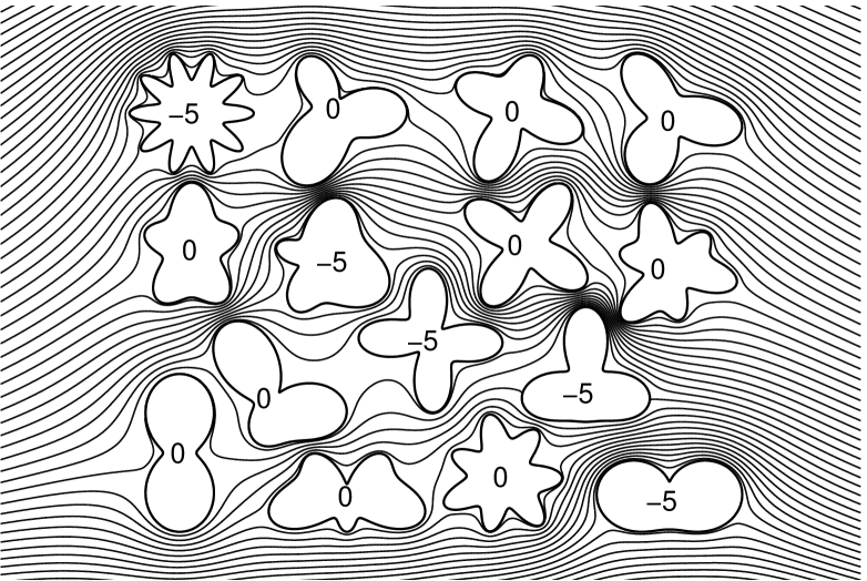
Figure 2: Numerical results for Example 1 obtained with $n=2048$ (total number of nodes is $30720$). The streamlines are shown for $\alpha=0$ and for zero circulations along $10$ aerofoils and non-zero circulations along $5$ aerofoils (the circulation along each aerofoils is shown inside the curve).

Example 2.

The region $G$ is an unbounded multiply connected region exterior to $110$ smooth Jordan curves (see Fig. 3).

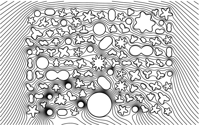
Figure 3: Numerical results for Example 2 obtained with $n=2048$ (total number of nodes is $225280$). The streamlines are shown for $\alpha=0$ and for circulations $-5$ along the cylindrical aerofoils and zero circulations along the other aerofoils.

Example 3.

The region $G$ is an unbounded multiply connected region exterior to $2000$ circles (see Fig. 4).

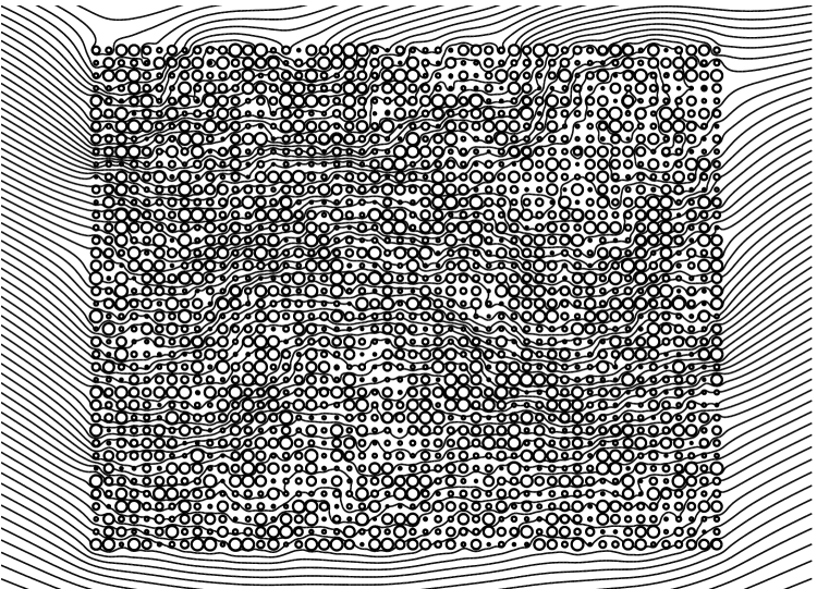
Figure 4: Numerical results for Example 3 obtained with $n=1024$ (total number of nodes is $2048000$). The streamlines are shown for $\alpha=0$ and the circulations along each aerofoil is an arbitrary number between $-1$ and $1$.

References

- [1] K. E. Atkinson. The Numerical Solution of Integral Equations of the Second Kind. Cambridge University Press, Cambridge, 1997.
- [2] L. Greengard and Z. Gimbutas. FMMLIB2D: A MATLAB toolbox for fast multipole method in two dimensions. Version 1.2, 2012. http://www.cims.nyu.edu/cmcl/fmm2dlib/fmm2dlib.html.
- [3] P. Henrici. Applied and Computational Complex Analysis, Vol. 3. John Wiley, New York, 1986.
- [4] T. Kambe. Elementary Fluid Mechanics. World Scientific, Singapore, 2007.
- [5] A. H. M. Murid and M. M. S. Nasser. Eigenproblem of the generalized neumann kernel. Bulletin of the Malaysian Mathematical Science Society, 26:13–33, 2003.
- [6] M. M. S. Nasser. A boundary integral equation for conformal mapping of bounded multiply connected regions. Comput. Methods Funct. Theory, 9:127–143, 2009.
- [7] M. M. S. Nasser. Numerical conformal mapping via a boundary integral equation with the generalized neumann kernel. SIAM J. Sci. Comput., 31(3):1695–1715, 2009.
- [8] M. M. S. Nasser. The riemann-hilbert problem and the generalized neumann kernel on unbounded multiply connected regions. The University Researcher (IBB University Journal), 20:47–60, 2009.
- [9] M. M. S. Nasser. Boundary integral equations for potential flow past multiple aerofoils. Comput. Methods Funct. Theory, 11:375–394, 2011.
- [10] M. M. S. Nasser. Numerical conformal mapping of multiply connected regions onto the second, third and fourth categories of koebe’s canonical slit domains. J. Math. Anal. Appl., 382:47–56, 2011.
- [11] M. M. S. Nasser. Numerical conformal mapping of multiply connected regions onto the fifth category of koebe’s canonical slit regions. J. Math. Anal. Appl., 398:729–743, 2013.
- [12] M. M. S. Nasser and F. A. A. Al-Shihri. A fast boundary integral equation method for conformal mapping of multiply connected regions. SIAM J. Sci. Comput., 35(3):A1736–A1760, 2013.
- [13] M. M. S. Nasser and A. H. M. Murid. Numerical experiments on eigenvalues of the generalized neumann kernel. In A.H.M. Murid and Y. Yaacob, editors, Advances in Group Theory, DNA Splicing and Complex Analysis, pages 135–158. Penerbit UTM Press, 2012.
- [14] M. M. S. Nasser, A. H. M. Murid, M. Ismail, and E. M. A. Alejaily. A boundary integral equation with the generalized neumann kernel for laplace’s equation in multiply connected regions. Appl. Math. Comput., 217:4710–4727, 2011.
- [15] M.M.S. Nasser. Fast solution of boundary integral equations with the generalized neumann kernel. In A.H.M. Murid and Y. Yaacob, editors, Recent Advances on Integral Equations with the Generalized Neumann Kernel. Penerbit UTM Press, Submitted.
- [16] Y. Saad and M. H. Schultz. Gmres: A generalized minimum residual algorithm for solving nonsymmetric linear systems. SIAM J. Sci. Stat. Comput., 7(3):856–869, 1986.
- [17] R. Wegmann, A. H. M Murid, and M. M. S. Nasser. The riemann-hilbert problem and the generalized neumann kernel. J. Comput. Appl. Math., 182:388–415, 2005.
- [18] R. Wegmann and M. M. S. Nasser. The riemann-hilbert problem and the generalized neumann kernel on multiply connected regions. J. Comput. Appl. Math., 214:36–57, 2008.