Griffiths phases and the stretching of criticality in brain networks

Abstract

Hallmarks of criticality, such as power-laws and scale invariance, have been empirically found in cortical networks and it has been conjectured that operating at criticality entails functional advantages, such as optimal computational capabilities, memory, and large dynamical ranges. As critical behavior requires a high degree of fine tuning to emerge, some type of self-tuning mechanism needs to be invoked. Here we show that, taking into account the complex hierarchical-modular architecture of cortical networks, the singular critical point is replaced by an extended critical-like region which corresponds –in the jargon of statistical mechanics– to a Griffiths phase. Using computational and analytical approaches, we find Griffiths phases in synthetic hierarchical networks and also in empirical brain networks such as the human connectome and the caenorhabditis elegans one. Stretched critical regions, stemming from structural disorder, yield enhanced functionality in a generic way, facilitating the task of self-organizing, adaptive, and evolutionary mechanisms selecting for criticality.

Empirical evidence that living systems can operate near critical points is flowering in contexts ranging from gene expression patterns Kauffman08 , to optimal cell growth Kaneko , bacterial clustering Chen-bacteria , or flocks of birds Cavagna12 . In the context of neuroscience, synchronization patterns have been shown to exhibit broadband criticality broadband , critical avalanches of spontaneous neural activity have been consistently found both in vitro BP03 ; Plenz07 ; Beggs08 and in vivo Peterman09 , and results from large-scale brain models based on the human connectome show that only at criticality the brain structure is able to support the dynamics seen in functional magnetic resonance imaging (fMRI) recordings Haimovici . All this evidence suggests that criticality – with its concomitant power laws and scale invariance – might play a relevant role in intact-brain dynamics Beggs08 ; Chialvo10 . At variance with inanimate matter – for which the emergence of generic or self-organized criticality in sandpile models, type-II superconductors, or solar flares is relatively well understood, Bak ; SOC-Jensen ; BJP – criticality in living systems can be conjectured to be the result of evolutionary or adaptive processes, which for reasons to be understood select for it.

The criticality hypothesis Beggs08 ; Chialvo10 ; Mora-Bialek states that biological systems can perform the complex computations that they require to survive only by operating at criticality (the edge of chaos), i.e. at the borderline between an active or chaotic phase in which noise propagates unboundedly—thereby corrupting all information processing or storage—and a quiescent or ordered phase in which perturbations readily fade away, hindering the ability to react and adapt Langton ; Ber-Nat . Critical dynamics provides a delicate trade-off between these two impractical tendencies, and it has been argued to imply optimal transmission and storage of information Haldeman05 ; Plenz07 ; Beggs08 , optimal computational capabilities Legenstein07 , large network stability Ber-Nat , maximal variety of memory repertoires BP04 , and maximal sensitivity to stimuli Kinouchi-Copelli .

Such a delicate balance occurs just at a singular or critical point, requiring a precise fine tuning. However, a very recent fMRI analysis of the human brain at its resting state, reveals that the brain spends most of the time wandering around a broad region near a critical point, rather than just sitting at it Taglia . This suggests that the region where cortical networks operate is not just a critical point, but a whole extended region around it.

Here, inspired by this empirical observation as well as by some recent findings in network theory and neuroscience GPCN ; Rubinov ; Zhou12 we scrutinize the dynamics of simple models of neural activity propagation when the structural architecture of brain networks is explicitly taken into account. Using a combination of analytical and computational tools, we show that the intrinsically disordered (hierarchical and modular) organization of brain networks dramatically influences the dynamics by inducing the emergence – in the jargon of Statistical Mechanics – of a Griffiths phase (GP) Griffiths ; Noest ; Vojta-Review ; GPCN . This phase, which stems from the presence of disorder (structural heterogeneity here) is characterized by generic power-laws extending over broad regions in parameter space. Furthermore, functional advantages usually ascribed to criticality, such as a huge sensitivity to stimuli, are reported to emerge generically all along the GP. Remarkably, not only do we find GPs in stylized models of brain architecture, but also in real neural networks such as those of the C. elegans and the human connectome.

Our conclusion is that, as a consequence of the intrinsically-disordered architecture of brain networks, critical-like regions are extended from a singular point to a broad or stretched region, much as evidenced in recent fMRI experiments. The existence of Griffiths phases facilitates the task of self-organizing, adaptive, or evolutive mechanisms seeking for critical-like attributes, with all their alleged functional advantages.

We claim that the intrinsic structural heterogeneity of cortical networks calls for a change of paradigm from the critical/edge-of-chaos to a new one, relying on extended critical-like Griffiths regions. Our work also raises a series of questions worthy of future pursuit. For instance, is there any connection between GPs and the empirically reported generic power-law decay of short-time memories? Do our results extend to other hierarchical architectures such as those encountered in metabolic or technological networks?

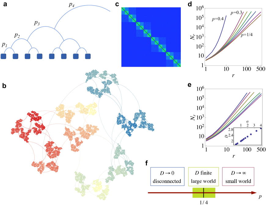
Figure 1: Hierarchical modular networks. (a) Sketch of the bottom-top approach (HMN-1 model): initially, nodes are grouped into fully connected modules of size ${\it M}_{\textrm{0}}$ (blue squares); then nodes in different modules are clustered recursively into sets of ${\it b}$ higher level blocks (e.g. in pairs, ${\it b}=2$) linking their respective nodes with hierarchical-level dependent wiring probabilities (HMN-1): ${\it p}_{\textrm{l}}={\it\alpha}{\it p}^{l}$ with $0<{\it p}<1$ and ${\it\alpha}$ a constant. At level ${\it l}$, each of the existing ${\it N}/2^{l}$ pairs is connected on average by ${\it n}_{\textrm{l}}=4^{l}({\it M}_{\textrm{0}}/2)^{2}\times{\it\alpha p}^{l}$ links. The resulting networks are always connected; with total number of ${\it N}={\it M}_{\textrm{0}}\times{\it b}^{s}$ nodes, and average connectivity ${\it k}=({\it M}_{\textrm{0}}-1)+{\it\alpha}({\it M}_{\textrm{0}}/2)\sum_{i=1}^{s}(2{\it p})^{i}$. (b) Graph representation of a HMN-1 with ${\it N}=2^{11}$ nodes, organized across ${\it s}=10$ hierarchical levels (${\it M}_{\textrm{0}}=2$, ${\it p}=1/4$, and ${\it\alpha}=4$). (c) Adjacency matrix of the connection-density (as in b) averaged over several network realizations (greener for larger densities). (d and e) Topological dimension, ${\it D}$, as defined by ${\it N}_{\it r}\sim{\it r}^{D}$ (see main text) as a function of parameters. (d) As ${\it p}$ is increased ${\it D}$ (the slope of the straight lines in the double logarithmic plot) grows and eventually becomes infinite; for smaller values of ${\it p}$ (not shown) it becomes flat, and ${\it D}\rightarrow 0$. (e) keeping ${\it p}=1/4$, the topological dimension ${\it D}$ is finite and continuously varying as function of ${\it\alpha}$, (values summarized in the inset). (f) Summary of structural properties: networks are disconnected (vanishing topological dimension, ${\it D}$) and small-world (${\it D}=\infty$) for small and large values of ${\it p}$ respectively, while around ${\it p}=1/4$ networks have a finite ${\it D}$ (as well as a finite connectivity and a finite density of connections in the large-${\it N}$ limit, i.e. networks are scalable).

I Results

I.1 Hierarchical network architectures

The cortex network has been the focus of attention in neuroanatomy for a long time, but only recently, the development of high-throughput methods has allowed the unveiling of its intricate architecture or connectome Hagmann ; Honey09 . Brain networks have been found to be structured in moduli –each modulus being characterized by having a much denser connectivity within it than with elements in other moduli– organized in a hierarchical fashion across many scales Sporns ; Review-Kaiser ; Review-Bullmore . Moduli exist at each hierarchical level: cortical columns arise at the lowest level, cortical areas at intermediate ones, and brain regions emerge at the systems level, forming a sort of fractal-like nested structure Sporns ; Review-Kaiser ; Review-Bullmore ; SCKH .

To be able to perform systematic analyses, we have designed synthetic hierarchical and modular networks (HMN) with ${\it s}$ hierarchical levels, ${\it N}$ nodes/neurons, and ${\it L}$ links/synapses, whose structure can be tuned to mimic that of real networks. We employ two different HMN models based on a bottom-top approach; in the first, local fully-connected moduli are constructed and then recursively grouped by establishing new inter-moduli links between them in either a stochastic way with a level-dependent probability ${\it p}$ as sketched in Figure 1 (HMN-1) section or in a deterministic way with a level-dependent number of connections (HMN-2). For further details see the Materials and Methods (MM) section. Similarly, top-down models can also be designed Zhou11 .

A way to encode key network structural information is the topological dimension, ${\it D}$, which measures how the number of neighbors of any given node grows when moving $1$, $2$, $3$, …, ${\it r}$ steps away from it: ${\it N_{r}}\sim{\it r}^{D}$ for large values of ${\it r}$. Networks with the small-world property Barabasi-Review have local neighborhoods quickly covering the whole network, i.e. ${\it N_{r}}$ grows exponentially with ${\it r}$, formally corresponding to ${\it D}\rightarrow\infty$. Instead, large-worlds have a finite topological dimension, while ${\it D}=0$ describes fragmented networks (see Figure 1). Our synthetic HMN models span all the spectrum of ${\it D}$-values as illustrated in Figure 1.

Strictly speaking, the HMN networks that we will consider in the following are finite dimensional only for ${\it p}=1/4$, in which case the number of inter-moduli connection is stable across hierarchical levels (see MM). For ${\it p}>1/4$ (resp. ${\it p}<1/4$) networks become more and more densely (resp. sparsely) connected as the hierarchy depth (i.e. the network size) is increased. Deviations from ${\it p}=1/4$ create fractal-like networks up to certain scale, being good approximations for finite-dimensional networks in finite size. In some works (e.g. PNAS-Gallos ), the Hausdorff (fractal) dimension ${\it D}_{\textrm{f}}$ is computed for complex networks. We have verified numerically that ${\it D}_{\textrm{f}}\approx{\it D}$ in all cases for HMNs.

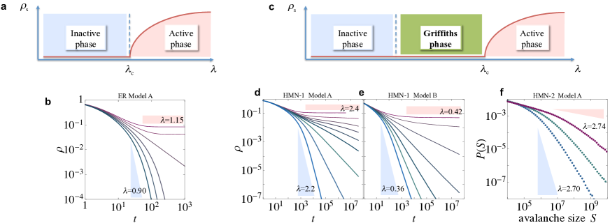
Figure 2: Conventional versus non-conventional phase diagram. Left: (a and b) conventional critical point scenario for our Model A running upon a random Erdős-Rényi network ($10^{6}$ nodes, average connectivity $20$, infinite topological dimension ${\it D}$): a singular power-law separates a quiescent phase (with exponential decay) from an active one (with a non-trivial steady state). Right: (c–f) Emergence of broad regions of power-law scaling in HMNs. (c) Schematic phase diagram for a system exhibiting a broad region of power-law scaling. The stationary density of activity, ${\it\rho}_{\textrm{s}}$, is depicted as a function of the spreading rate ${\it\lambda}$. (d and e) Steady state density of active sites, for Model-A and Model-B dynamics respectively, on HMN-1 networks (with ${\it N}=2^{14}$ nodes, and parameters ${\it s}=13$, ${\it p}=1/4$, ${\it\alpha}=1$). Data for increasing values of the spreading rate ${\it\lambda}$, from bottom to top. (f) Avalanche-size distributions for Model A on a HMN-2 network (${\it N}=2^{14}$, ${\it s}=13$, ${\it p}=1/4$, ${\it\alpha}=1$; Griffiths phase for such networks is observed for $2.60\leq{\it\lambda}\leq 2.79$); avalanche sizes are power-law distributed over a wide range ${\it\lambda}$ values reflecting the existence of a GP. These conclusions have been confirmed in finite-size scaling analyses, and can be generalized for other combinations of network architectures and dynamical models.

I.2 Architecture-induced Griffiths phases

Disorder is well-known to radically affect the behavior of phase transitions (see Vojta-Review and refs. therein). In disordered systems, there exist local regions characterized by parameter values which differ significantly from their corresponding system averages. Such rare regions can, for instance, induce the system to be locally ordered, even if globally it is in the disordered phase. In this way, in propagation-dynamic models, activity can transitorily linger for long times within rare active regions, even if the system is in its quiescent phase. In the particular case in which broadly different rare-regions exist – with broadly distinct sizes and time-scales – the overall system behavior, determined by the convolution of their corresponding highly-heterogeneous contributions, becomes anomalously slow (see Section I.3). In contrast with standard critical points, systems with rare-region effects have an intermediate broad phase separating order from disorder: a Griffiths phase (GP) with generic power-law behavior and other anomalous properties (e.g. Vojta-Review and Section I.3)

Remarkably, it has been very recently shown that structural heterogeneity can play in networked systems a role analogous to that of standard quenched disorder in physical systems GPCN . In particular, simple dynamical models of activity propagation exhibit GPs when running upon networks with a finite topological dimension ${\it D}$. On the other hand, in small-world networks (with ${\it D}=\infty$) local neighborhoods are too large – quickly covering the whole network – as to be compatible with the very concept of rare (isolated) regions GPCN . Therefore, it has been conjectured that a finite topological dimension ${\it D}$ is an excellent indicator of eventual rare-region effects and GPs.

I.3 Anomalous propagation dynamics in HMNs

To model the propagation of neuronal activity, we consider highly-simplified dynamical models running upon HMNs. More realistic models of neural dynamics with additional relevant layers of information could be considered; but we do not expect them to significantly affect our conclusions. Our approach here consists in modeling activity propagation in a minimal way; in some of the cases that we study, the network nodes are not neurons but coarse neural regions, for which effective models of activity propagation are expected to provide a sound description of large-scale properties. Every node (or neuron) is endowed with a binary state variable ${\it\sigma}$, representing either activity (${\it\sigma}=1$) or quiescence (${\it\sigma}=0$). Each active neuron is spontaneously deactivated at some rate ${\it\mu}$ (${\it\mu}=1$ here), while it propagates its activity to other directly connected neurons at rate ${\it\lambda}$. We have considered two different dynamics: in the first one, (Model A) a synapsis between an active and a quiescent node is randomly selected at each time and proved for activation, while in the other variant (Model B) a neuron is selected and all its neighbors are proved for activation. Details of the computational implementation of the two models, known in statistical physics as the contact process and the SIS model respectively, can be found in MM.

In general, depending on the value of $\lambda$ these models can be either in an active phase –for which the density ${\it\rho}$ of active nodes reaches a steady-state value ${\it\rho}_{\textrm{s}}>0$ in the large system-size and large-time limit– or in the inactive phase in which ${\it\rho}$ falls ineluctably in the quiescent configuration (${\it\rho}_{\textrm{s}}=0$). Separating these two regimes, at some value, ${\it\lambda}_{\textrm{c}}$, there is a standard critical point where the system exhibits power-law behavior for quantities of interest, such as the time decay of a homogeneous initial activity density, ${\it\rho(t)}\sim{\it t}^{-\theta}$, or the size-distribution of avalanches triggered by an initially localized perturbation, $P({\it S})\sim{\it S}^{-\tau}$. Here ${\it\theta}$ and ${\it\tau}$ are critical indices or exponents. This standard critical-point scenario (see Figures 2a and 2b) holds for regular lattices, Erdős-Renyi networks, and many other types of networks. On the other hand, computer simulations of the different dynamical models running upon our complex HMN topologies with finite ${\it D}$ reveal a radically different behavior (see Figure 2c–2f and MM). The power-law decay of the average density ${\it\rho(t)}$ – specific to the critical point in pure systems – extends to a broad range of ${\it\lambda}$ values. The existence of a broad interval with power-law decaying activity is supported by finite size scaling analyses reported in MM. Likewise, as shown in Figure 2f, avalanches of activity generated from a localized seed have power-law distributed sizes, with continuously varying exponents, in the same broad region. These features are fingerprints of a GP and have been confirmed to be robust against increasing system size (up to ${\it N}=2^{20}$), using different types of HMN (HMN-1 with different values of ${\it\alpha}$ and ${\it p}$, HMN-2 models, all with finite ${\it D}$) and dynamical models (see MM).

How do Griffiths phases work? For illustration purposes, let us consider a simplified example. Consider Model A (the contact process) on a generic network, with a node-dependent quenched spreading rate ${\it\lambda}({\bf x})$, characterized –without loss of generality– by a bimodal distribution of $\lambda$ with average value $\bar{{\it\lambda}}$. Suppose the two possible values of $\lambda$ are one above and one below the critical point of the pure model, ${\it\lambda}_{\textrm{c}}$. In this way, at each location the system has an intrinsic preference to be either in the active or in the quiescent phase. Under these circumstances, typically, ${\it\lambda}_{\textrm{c}}<\bar{{\it\lambda}}_{\textrm{c}}$, so that, for values of $\bar{{\it\lambda}}$ in between ${\it\lambda}_{\textrm{c}}$ and $\bar{{\it\lambda}}_{\textrm{c}}$ the disordered system is in its quiescent phase. However, there are always spatial locations characterized by significantly over-average values of (actually, local values of ${\it\lambda}({\bf x})>{\it\lambda}_{\textrm{c}}$). In these regions, initial activity can linger for very long periods, especially if they happen to be large. Still, as such rare regions have a finite size, they ineluctably end up falling into the inactive state. Considering a rare active region of size ${\it\zeta}$, it decays to the quiescent state after a typical time ${\it\tau(\zeta)}$, which grows exponentially with cluster size, i.e. ${\it\tau}\simeq t_{\textrm{0}}\exp[{\it A(\lambda)\zeta]}$ (Arrhenius law), where ${\it t}_{\textrm{0}}$ and ${\it A(\lambda)}$ do not depend on ${\it\zeta}$. On the other hand, the distribution of ${\it\zeta}$-values is also exponential (very large regions are exponentially rare). Therefore, the overall activity density, ${\it\rho(t)}$, decays as the following convolution integral

$${\it\rho(t)}\sim\int d{\it\zeta}P({\it\zeta}){\it\zeta}\exp{[-{\it t}/({\it t}_{\textrm{0}}e^{A(\lambda)\zeta})]},$$ (1)

which evaluated in saddle-point approximation leads to ${\it\rho(t)}\sim{\it t}^{-\theta}$, with ${\it\theta}(\bar{{\it\lambda)}}$ varying continuously with the disorder average value, $\bar{{\it\lambda}}$. Such generic power laws signal the emergence of Griffiths phases. This is just an explanatory example of a general phenomenon, thoroughly studied in classical, quantum, and non-equilibrium disordered systems Vojta-Review . In HMNs, the quenched disorder is encoded in the intrinsic disorder of the hierarchical contact pattern.

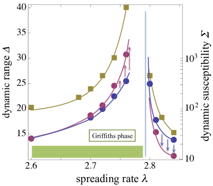
Figure 3: Network response diverges all along the Griffiths phase. Right axis: dynamic susceptibility, ${\it\Sigma}$, measured for the dynamical Model A in HMN-2 networks of size ${\it N}=2^{14}$ (blue circles) and ${\it N}=2^{17}$ (purple circles); the critical point ${\it\lambda}_{\textrm{c}}\approx 2.79$, is marked as a vertical line (see MM: dynamical protocol iii). In the GP (resp. active phase) the overall response increases (resp. decreases) for larger systems as marked by the red (resp. blue) arrows. In the GP, ${\it\Sigma}$ grows as a ${\it\lambda}$-dependent power-law of ${\it N}$. Left axes: dynamic range ${\it\Delta}$ (green squares) for the same case as above, ${\it N}=2^{14}$ (dynamical protocol iv; see MM). Instead of the usual symmetric cusp-singularity at the critical point, there is a whole region of extremely large ${\it\Delta}$ with a strong asymmetry around the transition point, as corresponds to the existence of a GP.

I.4 Diverging response in HMNs

One of the main alleged advantages of operating at criticality is the strong enhancement of the system’s ability to distinctly react to highly diverse stimuli. In the statistical mechanics jargon this stems from the divergence of the susceptibility at criticality Binney . How do systems with broad GPs respond to stimuli? To answer this question we measure the following two different quantities (see MM):

(i) The dynamic susceptibility gauges the overall response to a continuous localized stimulus and is defined as ${\it\Sigma(\lambda)}={\it N}[{\it\rho}_{\textrm{f}}({\it\lambda})-{\it\rho}_{\textrm{s}}({\it\lambda})]$, where ${\it\rho}_{\textrm{s}}({\it\lambda})$ is the stationary density in the absence of stimuli and ${\it\rho}_{\textrm{f}}({\it\lambda})$ is the steady-state density reached when one single node is constrained to remain active. As shown in Figure 3, ${\it\Sigma}$ becomes extremely large in the GP and, more importantly, it grows as a power-law of system-size, ${\it\Sigma}({\it\lambda}\approx{\it\lambda}_{\textrm{c}},{\it N})\sim{\it N}^{\eta}$, implying that there is an extended extended region (the whole GP) where the system exhibits a divergent response (with ${\it\lambda}$-dependent continuously varying exponents)

(ii) The dynamic range, ${\it\Delta}$, introduced in this context in Kinouchi-Copelli , measures the range of perturbation intensities/frequencies for which the system reacts in distinct ways, being thus able to discriminate among them. We have computed ${\it\Delta}({\it\lambda})$ in the HMN-2 model (see Figure 3) which clearly illustrates the presence of a broad region with huge dynamic ranges (rather than the standard situation for which large responses are sharply peaked at criticality).

Therefore, if critical-like dynamics is important to access a broad dynamic range and to enhance system’s sensitivity, then it becomes much more convenient to operate with hierarchical-modular systems, where criticality – with extremely large responses and huge sensitivity – becomes a region rather than a singular point.

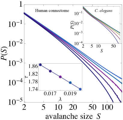
Figure 4: Critical avalanches all along the Griffiths phase in real brain networks. Avalanche-size statistics for Model-B dynamics in real neural networks. Main plot: human connectome network (consisting of $998$ brain areas and the structural connections among them). Avalanche-size distributions for Model-B dynamics (with $0.016\leq\lambda\leq 0.020$ equispaced values). Truncated power-laws $P({\it S})\sim{\it S}^{-\tau}e^{-S/\xi}$ with continuously varying exponents ${\it\tau}$ constitute the most reliable fits according to the Kolmogorov-Smirnoff criterion (see MM). Lower inset: The ${\it\tau}$ exponent (estimated through non-linear least-square fits) as a function of ${\it\lambda}$; it converges to $\approx 1.7$ at the critical point, ${\it\lambda}_{\textrm{c}}\approx 0.020$. Upper inset: as the main figure but for the C. elegans neural network ($0.08\leq{\it\lambda}\leq 0.12$).

I.5 Griffiths phases in real networks

Analyses of different nature have revealed that organisms from the primitive C. elegans Review-Bullmore ; Review-Kaiser ; Sinha ; Varshney (for which a full detailed map of its about $300$ neurons has been constructed) to cats, macaque monkeys, or humans (for which large-scale connectivity maps are known Hagmann ) have a hierarchically organized neural network. Such structure is also shared by functional brain networks (e.g. from functional magnetic resonance imaging data) Zhou06 ; PNAS-Gallos ; Hagmann ; Honey09 ; Bassett10 . Do simple dynamical models of activity propagation (such as those in previous sections) running upon real neural networks exhibit GPs?

We have considered the human connectome network, obtained by Sporns and collaborators using diffusion imaging techniques Hagmann ; Honey09 . It consists of a highly coarse-grained mapping (as opposed for instance to the detailed map of C. elegans) of anatomical connections in the human brain, comprising ${\it N}=998$ brain areas and the fiber tract densities between them, with a hierarchical organization Review-Bullmore ; Review-Kaiser (see MM).

Given that this network comprises only ${\it N}\lesssim 1000$ nodes, the maximum size of possible rare regions and the associated power laws are necessarily cut-off at small sizes and short times. Nevertheless, as illustrated in Figure 4, simulations of the dynamical models above (Model B in this case) show a significant deviation from the typical standard critical-point scenario. Instead, avalanches are clearly distributed as power laws, with moderate finite-size effects, in a broad range of ${\it\lambda}$-values (see Figure 4). Actually, truncated power-laws of the form $P({\it S})\sim{\it S}^{-\tau}e^{-S/\xi}$ – with ${\it\lambda}$-dependent values of ${\it\tau}$ – provide highly reliable fits of the size distributions, $P({\it S})$, according to the Kolmogorov-Smirnoff criterion (see MM), supporting the picture of a broad critical-like region. This strongly suggests that if it were feasible to run dynamical models upon the actual human brain network (with about $10^{12}$ neurons and $10^{15}$ synapses) a GP would appear in a robust way, and would extend over much larger range of size and time scales. Similar results, even if affected by more severe size effects, are obtained for the C. elegans detailed neural network, consisting of ${\it N}\lesssim 300$ neurons (see Figure 4, upper inset).

I.6 Spectral fingerprints of Griffiths phases in HMNs

To further confirm the existence of Griffiths phases (beyond direct computational simulations), here we present some analytical results. An important tool in the analysis of network dynamics is provided by spectral graph theory, in which the network structure is encoded in some matrix and linear algebra techniques are exploited FanChung . For instance, the dynamics of simple models (e.g. Model-B) is often governed by the largest (or principal) eigenvalue, ${\it\Lambda}_{\textrm{max}}$, of the adjacency matrix, ${\it A}_{ij}$ (with $1$’s as entries for existing connections and $0$’s elsewhere), which straightforwardly appears in a standard linear stability analysis (as detailed in the MM section). It is easy to show that (with very mild assumptions) the critical point –signaling the limit of linear stability of perturbations on the quiescent state– is given by ${\it\lambda}_{\textrm{c}}{\it\Lambda}_{\textrm{max}}=1$. Remarkably, it has been recently shown that this general result may not hold for certain networks, for which the largest eigenvalue has an associated localized eigenvector (i.e. with only a few non-vanishing components; this phenomenon closely resembles Anderson localization in physics Goltsev12 ). In such a case, linear instabilities for ${\it\lambda}$ slightly larger than $1/{\it\Lambda}_{\textrm{max}}$ lead to localized activity around only few nodes (where the corresponding eigenvector is localized), not pervading the network and not leading to a true active state. This implies that the critical point is shifted to a larger value of ${\it\lambda}$. Instead, these regions of localized activity resemble very much rare-regions in GPs: activity lingers around them until eventually a large fluctuation kills them.

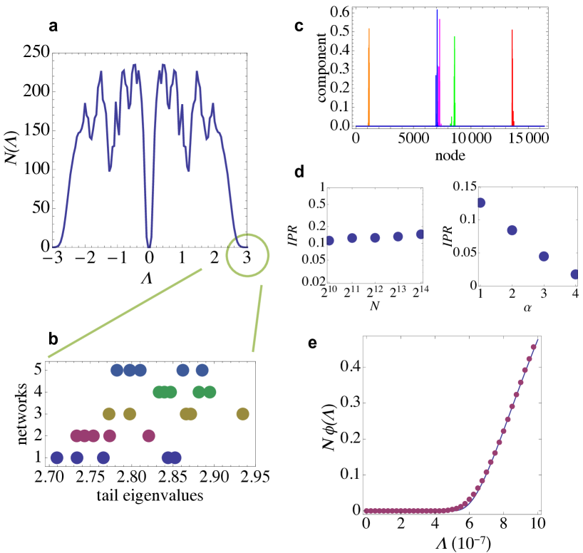
Figure 5: Spectral analyses of hierarchical networks. (a) Average spectrum of the adjacency matrix of HMN-2 networks (${\it N}=2^{14}$, ${\it s}=13$, ${\it M}_{\textrm{0}}=2$, ${\it\alpha}=1$). Data are averaged over $150$ network realizations. The vertical axis reports the average number of eigenvalues (not the density). (b) Ideal zoom of the higher spectral edge of (a). The values of the $5$ largest eigenvalues for $5$ randomly chosen networks from (a) are represented. No proper spectral gap is observed. (c) Localization of the $5$ eigenvectors corresponding to the largest eigenvalues. The principal eigenvector ${\bf f}({\it\Lambda}_{\textrm{max}})$ is plotted in red. Being our HMNs connected, in agreement with the Perron-Frobenius theorem gantmacher the components of ${\bf f}({\it\Lambda}_{\textrm{max}})$ (even the vanishing ones) are all strictly positive, although this cannot be appreciated in linear scale. The next eigenvectors are plotted in magenta, orange, green and blue. (d) Dependence of the IPR on the system size and the number of block-block connections in HMN-2 networks. (e) Lower spectral edge of the cumulative distribution of Laplacian eigenvalues of HMN-2 networks as in (a). Numerical data (points) are compared to an exponential Lifshitz tail with exponent ${\it a}\approx 1.00$. The Laplacian matrix is defined as ${\it L}_{ij}=\sum_{k}A_{ik}-A_{ij}$.

Inspired by this novel idea, we performed a spectral analysis of our HMNs (e.g. HMN-2 nets with ${\it\alpha}=1$, see Figure 5), with the result that – for finite ${\it D}$ networks – not only the largest eigenvalue ${\it\Lambda}_{\textrm{max}}$ corresponds to a localized eigenvector, but a whole range of eigenvalues below ${\it\Lambda}_{\textrm{max}}$ (even hundreds of them) share this feature, as can be quantitatively confirmed (see Figure 5c-d and MM). In particular, the principal eigenvector is heavily peaked around a cluster of neighboring nodes. We have conjectured and verified numerically that the clusters where the largest eigenvalues are localized correspond to the rare-regions, with above-average connectivity and where localized activity lingers for long time. Also, we numerically found ${\it\lambda}_{\textrm{c}}\approx 0.41>1/\Lambda_{\textrm{max}}\approx 0.33$, confirming the prediction above. The interval between these two values defines the GP (see MM).

In addition, we also considered large network ensembles and computed the probability distribution of eigenvalues. We found that the distribution of the eigenvalues corresponding to localized eigenvectors results in an exponential tail of the continuum spectrum, where an infinite dimensional graph would exhibit a spectral gap instead (see MM). This translates into an exponential tail of the cumulative distribution $\phi({\it\Lambda})$ of Laplacian eigenvalues (or integrated density of states) at the lower spectral edge, a so-called Lifshitz tail – which in equilibrium systems is related to the Griffiths singularity Nie . We have found Lifshitz tails with their characteristic form

$$\phi({\it\Lambda})\propto\exp\left[-\frac{1}{({\it\Lambda}-{\it\Lambda_{\textrm{min}}})^{a}}\right]$$ (2)

(where $a$ is a real parameter, see Figure 5e). Interestingly, Lifshitz tails are also rigorously predicted on Erdős Rényi networks below the percolation threshold, where rare-region effects and Griffiths phases are an obvious consequence of the network disconnectedness Khorunzhiy06lifshitstails . Therefore, the presence of both (i) localized eigenvectors and (ii) Lifshitz tails confirms the existence of GPs in networks with complex heterogeneous architectures.

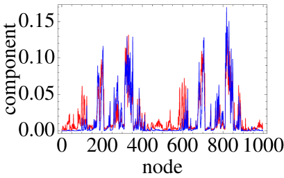
Figure 6: Localization properties of the human connectome network. Principal eigenvector of the weighted (blue) and unweighted (red) adjacency matrix. As the peak structure is roughly preserved, localization properties are expected to be alike in the two representations. In both cases regions of localized activity are evident.

The fingerprints of extended criticality in the human connectome are a result of its hierarchical network structure, and the localization properties that characterize it. Figure 6 supports this view, highlighting the localization of the principal eigenvector. In particular, we show that the principal eigenvector of the full adjacency matrix and that of the unweighted (i.e. with $1$’s as entries in correspondence to every non-zero weight) version of it display very similar peak structures (i.e. their rare regions are very similar). This last observation supports our choice to run simple unweighted dynamics on top of the connectome network. Connection weights will certainly contribute to a fully realistic description of the brain function, but they are not necessary in order to achieve broad criticality, which primarily arises from structural disorder.

II Discussion

A few pioneering studies have recently explored the role of hierarchical modular networks (HMN) on different aspects of neural dynamics. Rubinov et al. Rubinov argued that HMNs play a crucial role in fostering the existence of critical dynamics. Similar observations have been also made for spreading dynamics Kaiser07 ; Muller08 ; Zhou11 and for self-organization models Zhou12 , but so far these remain empirical findings lacking a satisfactory explanation.

Aimed at shedding light on these issues, here we have made the conjecture that owing to the intrinsically heterogeneous (i.e. disordered) architecture of brain HMNs and their large-world nature (which implies finite topological dimensions ${\it D}$), Griffiths phases are expected to emerge. These are characterized by broad regions in parameter space exhibiting critical-like features and, thus, not requiring of a too-precise fine tuning. To confirm this claim, we use a combination of computational tools and analytical arguments. In particular, we have constructed different synthetic HMNs covering a broad range of architectures (with either large- or small-world properties). For large worlds (i.e. finite topological dimension ${\it D}$), we find (i) generic anomalous slow relaxation and power-law distributed avalanches (with continuously varying exponents) in a broad region comprised between the active and the inactive phase; (ii) the system’s response to stimuli (as measured by the dynamic susceptibility and the dynamic range) is anomalously large: it diverges with system size through the whole GP. At a theoretical level, graph-spectral analyses reveal the presence of localized eigenvectors and Lifshitz tails which are the spectral counterparts of rare regions and GPs. All these evidences confirm the existence of GPs in synthetic HMNs, including a spectral graph theory viewpoint, thereby going beyond previous results in generic complex networks GPCN .

More remarkably, we have also provided evidence that GPs appear in actual real networks such as those of the human connectome and C. elegans, even if owing to the limited available network-sizes the associated power-laws are necessarily cut-off. Still, the best fits to data are provided by continuously varying power-laws, truncated by finite-size effects.

It is noteworthy that disorder needs to be present at very different scales for GPs to emerge (otherwise rare regions cannot be arbitrarily large); this is why a hierarchy of levels is required. Plain modular networks – without the broad distribution of cluster sizes, characteristic of hierarchical structures – are not able to support GPs. We emphasize that GPs in HMNs are induced merely by the existence of structural disorder: no additional form of neuronal or synaptic heterogeneity has been considered here; adding further heterogeneity would only enhance rare-region effects and hence GPs. For instance, we have also found GPs for the human connectome, when taking into account the relative weight of structural connections. It should also be noticed that all networks in our study are undirected in the sense that links are symmetrical, while synapses in cortical networks are not. Again, this does not jeopardize our conclusions: directness in the connections only strengthens isolation and hence rare-region effects and GPs.

The existence of a GP with its concomitant generic power-law scaling – not requiring a delicate parameter fine tuning – provides a more robust and solid basis to justify the ubiquitous presence of scale-free behavior in neural data, from EEG or MEG records to neural avalanches. More in particular, it might give us the key to understanding why broad regions around criticality are observed in fMRI experiments of the brain resting state Taglia .

As we have shown, the system’s response is extremely large (and diverges upon increasing the network size) in a broad region of parameter space. This strongly facilitates the task of mechanisms selecting for the alleged virtues of scale-invariance and strongly suggests that a new paradigm is needed: a theory of self-organization/evolution/adaptation to the broad region separating order from chaos. In particular, GPs combined with standard mechanisms for self-organization Levina07 ; Millman ; JABO-2 are expected to account for the empirically found dispersion around criticality Taglia . This also invites the question of whether intrinsically disordered HMNs do indeed generically optimize transmission and storage of information, improve computational capabilities Legenstein07 , or significantly enhance large network stability Ber-Nat , without the need to invoke precise criticality.

Usually, brain networks are claimed to be small worlds; instead we have shown that large-world architectures are essential for GPs to emerge. A solution to this conundrum was provided by Gallos et al. PNAS-Gallos , who found that (functional) brain networks consist of a myriad of densely connected local moduli, which altogether form a large world structure and, therefore, are far from being small-world; however, incorporating weak ties into the network converts it into a small world preserving an underlying backbone of well-defined moduli. To this end, it is essential that networks have a finite Hausdorff or fractal dimension (see Figure 1 and PNAS-Gallos ), confirming that finite dimensionality is a crucial feature. In this way, cortical networks achieve an optimal balance between local specialized processing and global integration through their hierarchical organization. On the other hand, weak links are not expected to significantly affect the existence of GPs. Therefore, from this perspective, (i) achieving such an optimal balance and (ii) operating with critical-like properties, can be seen as the two sides of the same coin. This stresses the need to develop new models for the co-evolution of structure and function in neural networks.

It is noteworthy that a mechanism for robust working memory without synaptic plasticity has been put forward very recently Samuel . It heavily relies on the existence of heterogeneous local clusters of densely inter-connected neurons, where activity (memories) reverberates. Not surprisingly, this leads to power-law distributed fade-away times, which have been claimed to be the correlate of power-law forgetting Forgetting . This is an eloquent illustration of Griffiths phases at work.

Given that disorder is an intrinsic and unavoidable feature of neural systems and that neural-network architectures are hierarchical, Griffiths phases are expected to play a relevant role in many dynamical aspects and, hence, they should become a relevant concept in Neuroscience as well as in other fields such as systems biology, where HMNs play a key role Escherichia . We hope that our work contributes to this purpose, fostering further research.

III Materials and Methods

Synthetic hierarchical networks. HMN-1: At each hierarchical level ${\it l}=1,2,\ldots s$, pairs of blocks are selected, each block of size $2^{i-1}{\it M}_{\textrm{0}}$. All possible $4^{i-1}{\it M}_{\textrm{0}}^{2}$ undirected eventual connections between the two blocks are evaluated, and established with probability ${\it\alpha p}^{l}$, avoiding repetitions. With our choice of parameters we stay away from regions of the parameter space for which the average number of connections between blocks ${\it n}_{l}$ is less than one, as this would lead inevitably to disconnected networks (as rare-region effects would be a trivial consequence of disconnectedness, we work exclusively on connected networks, i.e. networks with no isolated components). Since links are established stochastically, there is always a chance that, after spanning all possible connections between two blocks, no link is actually assigned. In such a case, the process is repeated until, at the end of it, at least one link is established. This procedure enforces the connectedness of the network and its hierarchical structure, introducing a cutoff for the minimum number of block-block connections at $1$. Observe also that for ${\it M}_{\textrm{0}}=2$ and ${\it p}=1/4$, ${\it\alpha}$ is the target average number of block-block connections and $1+{\it\alpha}$ the target average degree. However, by applying the above procedure to enforce connectedness, both the number of connections and the degree are eventually slightly larger than these expected, unconstrained, values.

For the HMN-2, the number of connections between blocks at every level is a priori set to a constant value ${\it\alpha}$. Undirected connections are assigned choosing random pairs of nodes from the two blocks under examination, avoiding repetitions. Choosing ${\it\alpha}\geq 1$ ensures that the network is hierarchical and connected. This method is also stochastic in assigning connections, although the number of them (as well as the degree of the network) is fixed deterministically. In both cases, the resulting networks exhibit a degree distribution characterized by a fast exponential tail, as shown in Supplementary Figure S1.

Empirical brain networks. Data of the adjacency matrix of C. elegans are publicly available (see e.g. Review-Kaiser ). Different analyses have confirmed that this network has a hierarchical-modular structure (see e.g. Review-Bullmore ; Sinha ; Varshney ; Reese ; 2Vicsek ). In particular, in 2Vicsek a new measure is defined to quantify the degree of hierarchy in complex networks. The C. elegans neural networks is found to be $6$ times more hierarchical than the average of similar randomized networks. Connectivity data for the human connectome network have been recently obtained experimentally Hagmann ; Honey09 . In this case too, the network is hierarchical Review-Bullmore ; Bassett10 ; Taglia . Supplementary Figure S2 shows a graphical representation of its adjacency matrix, highlighting its hierarchical organization.

Dynamical models. In both cases (Model A and Model B), neurons are identified with nodes of the network and are endowed with a binary state-variable ${\it\sigma}=0,1$. The state of the system is sequentially updated as follows. A list of active sites is kept. Model A: At each step, an active node is selected and becomes inactive ${\it\sigma}=0$ with probability ${\it\mu/(\lambda+\mu)}$, while with complementary probability ${\it\lambda/(\lambda+\mu)}$, it activates one randomly chosen nearest neighbor provided it was inactive. Model B: At each step, an active node is selected and becomes inactive ${\it\sigma}=0$ with probability ${\it\mu/(\lambda+\mu)}$, while with complementary probability ${\it\lambda/(\lambda+\mu)}$, it checks all of its nearest neighbors, activating each of them with probability $0<{\it\lambda}<1$ provided it was inactive, then it deactivates. Both Model A and B have well-known counterparts in computational epidemiology, where they correspond to the contact process and the susceptible-infective-susceptible model respectively (see for instance Romu01 ). The value of similar minimalistic dynamic rules in Neuroscience was proven before, e.g. in Grinstein-Linsker . Results for real networks are obtained by running Model B dynamics on the unweighted version of the network. We have verified that the introduction of weights does not alter the qualitative picture obtained.

Dynamical protocols. We employ four different dynamical protocols: (i) Decay of a homogeneous state: all nodes are initially active and the system is let evolve, monitoring the density of active sites ${\it\rho(t)}$ as a function of time. (ii) Spreading from a localized initial seed: an individual node is activated in an otherwise quiescent network. It produces an avalanche of activity, lasting until the system eventually falls back to the quiescent state; the survival probability $P_{\textrm{s}}({\it t})$ is measured. The avalanche size ${\it S}$ is defined as the number of activation events that occur for the duration of the avalanche itself. The process is iterated and the avalanche size distribution $P({\it S})$ is monitored. (iii) Identical to (ii), except that the seed is kept active throughout the simulation (continuous stimulus). (iv) Identical to (ii), except that the seed node is subsequently reactivated with probability ${\it p}_{\textrm{stimulus}}=1-\exp(-{\it r}\,{\it\Delta t})$ for ${\it t}>0$ (Poissonian stimulus of rate ${\it r}$).

Measures of response. The standard method to estimate responses consisting in measuring the variance of activity in the steady state, would not provide a measure of susceptibility in the Griffiths region, where a steady state is trivial (quiescent). We define the dynamic susceptibility as ${\it\Sigma}({\it\lambda})={\it N}[{\it\rho}_{\textrm{f}}({\it\lambda})-{\it\rho}_{\textrm{s}}({\it\lambda})],$ where ${\it\rho}_{\textrm{f}}({\it\lambda})$ is the steady state reached when a single node is constrained to be active throughout the simulation and ${\it\rho}_{\textrm{s}}({\it\lambda})$ the steady state for protocol (i), i.e. in the absence of constraints. In the inactive state, ${\it\rho}_{\textrm{s}}({\it\lambda})=0$ while ${\it\rho}_{\textrm{f}}({\it\lambda})$ is finite but small (of the order of $1/{\it N}$) as the active node continuously fosters activity in its surroundings. In the active state, ${\it\rho}_{\textrm{s}}({\it\lambda})$ and ${\it\rho}_{\textrm{f}}({\it\lambda})$ are both large and again differ by a little amount (given by the fixed node and its induced activity) that vanishes for larger system sizes. Only in the parameter region where the response of the system is high, the little perturbation introduced by the constrained node produces a diverging response. This is found to occur throughout the Griffiths region (see Figure 3, main text), confirming the claim of an anomalous response over an extended range of the parameter ${\it\lambda}$.

An alternative measure of response is provided by the dynamic range ${\it\Delta}$, introduced in Ref. Kinouchi-Copelli . We determine ${\it\Delta}({\it\lambda})$ for various values of ${\it\lambda}$ in the Griffiths and active phases, as follows:

(i) a seed node is chosen and initially activated, but not constrained to be active; (ii) the dynamical model (A, B, $\ldots$) is run; (iii) if the dynamics selects the seed node, and it is found inactive, it is reactivated with probability ${\it p}_{\textrm{stimulus}}$; (iv) the steady-state density ${\it\rho}$ is recorded (due to the intermittent reactivation, a steady state depending on ${\it p}_{\textrm{stimulus}}$ is always reached, unless ${\it p}_{\textrm{stimulus}}$ is infinitesimal); (v) upon varying ${\it p}_{\textrm{stimulus}}$, the steady-state density ${\it\rho}$ varies continuously within a finite window. We identify the values ${\it\rho}_{0.1}$ and ${\it\rho}_{0.9}$, corresponding to the $10\%$ and $90\%$ values within such window, and call ${\it p}_{0.1}$ and ${\it p}_{0.9}$ the values of ${\it p}_{\textrm{stimulus}}$ leading to those values respectively; (vi) the dynamic range is calculated as ${\it\Delta}=10\log_{10}({\it p}_{0.9}/{\it p}_{0.1})$.

Notice that in the active phase ${\it\rho}_{0.1}$ reaches a finite steady state at exponentially large times in the limit ${\it\lambda}\to{\it\lambda}_{c}^{+}$. This makes the study of large systems very lengthy in that parameter region.

Extended regions of enhanced response are found also by running our simple dynamic protocols on the connectome network. A way to visualize the broadening of the critical region is presented in Supplementary Figure S3, where the density of active sites given a fixed active seed ${\it\rho}_{\textrm{f}}$ is plotted as a function of ${\it\lambda}$. The critical region broadens if compared to the case of a regular (disorder-free) lattice of the same size.

Finite-size scaling. In the standard critical point scenario – assuming the system sits exactly at the critical point but it runs upon a finite system (of linear size L) – the average density (order parameter) starting from an initially active configurations decays as ${\it t}^{-\theta}\times\exp(-{\it t/\tau(L)})$, where the cut-off time scales with system size, as ${\it\tau(L)n}\propto{\it L}^{z}$ (${\it z}$ the dynamic critical exponent), allowing us to perform collapse plots for different system sizes. Instead, in Griffiths phases, the cut-off time does not have an algebraic dependence on ${\it L}$; it is the largest cluster which is cut-off by ${\it L}^{d}$, and the corresponding escape/decay time from it grows like ${\it\tau(L)}\propto\exp({\it cL}^{d})$. Therefore, even for relatively small system sizes, such a cut-off is not observable in (reasonable) computer simulations: order-parameter-decay plots should exhibit power-law asymptotes without any apparent cut-off. On the other hand, the power-law exponent – which can be estimated from a saddle point approximation, dominated by the largest rare region – is severely affected by finite size effects. Therefore, summing up, while in standard critical points finite size effects maintain the critical exponent but visibly affect the exponential cut-offs, in Griffiths phases, apparent critical exponents are affected by finite-size corrections while exponential cut-offs are not observable. Unless otherwise specified, simulations on HMNs are for systems of size ${\it N}=2^{14}=16384$. Supplementary Figure S4 shows that upon increasing the system size (and the number of hierarchical levels accordingly), the picture of generic power-law decay of activity remains valid in the whole GP. One can observe that for each value of ${\it\lambda}$, the effective exponent tends to an asymptotic value, which is expected to hold in the large-network-size limit.

Avalanches in the human connectome. Unlike avalanches on synthetic HMNs, typically run on several ($10^{7}-10^{8}$) network realizations, avalanche statistics on the human connectome network is the result of a large number of avalanches ($>10^{9}$) on the unique network available. Such limitation explains the emergence of strong cutoffs in the avalanche-size distributions (see Figure 4). In the main text, we propose to fit avalanche size distributions with truncated power laws, reflecting the superposition of generic power-law behavior and finite-size effects. In order to assess the validity of our hypothesis, we resort to the Kolmogorov-Smirnov method, by which the best fit is provided by the fitting function $g({\it S})$, which minimizes the estimator

$${\it D}_{\textrm{KS}}=\max|G(S)-F(S)|,$$ (3)

where $G({\it S})$ is the cumulative distribution associated with $g({\it S})$ and $F({\it S})$ is the cumulative distribution of empirical data (simulation results, in our case).

In case of limited amount of empirical data, the use of diverse fitting techniques (least squares, maximum likelihood etc.) is advised, in order to avoid biases. However, given the abundance of data in our case, a non-linear least-squares fit provides a reliable estimate of parameters (note that a truncated power-law cannot be fit linearly by standards methods). We recall that the least-squares method is essentially a minimization problem: given a set of empirical data points $({\it x}_{i},{\it y}_{i})_{i=1,\ldots n}$ and a fitting function $g({\bf x},{\bf y},{\bf b})$ depending on a set of parameters ${\bf b}$, the fit is provided by the set of parameters that minimizes the function $\sum_{i=1}^{n}[{\it y}_{i}-g({\it x}_{i},{\bf b})]^{2}$. In the case of a linear regression, such minimization can be performed exactly. In the case of a non-linear fit, instead, the minimization has to be performed numerically.

For every value of ${\it\lambda}$ (every curve in Figure 4), we proceed as follows: (i) we provide a least-squares fit for the avalanche-size distribution, based upon the truncated power-law hypothesis and calculate the corresponding Kolmogorov-Smirnov ${\it D}_{\textrm{KS}}$; (ii) we repeat the above procedure for alternative candidate distributions (non-truncated power law and exponential) (iii) we compare the results for the ${\it D}_{\textrm{KS}}$ indicators and choose the hypothesis with the smallest ${\it D}_{\textrm{KS}}$ as the best fit. In Supplementary Figure S5 we provide an example of this procedure, as obtained from our data for ${\it\lambda}=0.017$. In this case, as in every other case examined, the truncated power law provides the best fit among the ones tested, both by the KS criterion and upon visual inspection. Notice that also the power-law hypothesis appears plausible to some extent, whereas the exponential hypothesis deviates significantly from the data, however one chooses the minimum avalanche size ${\it S}_{\textrm{min}}$ to fit. Special attention has been devoted to the choice of the lower bound ${\it S}_{\textrm{min}}$, as advised in Ref Clauset . Such a choice is usually made by visual inspection for large systems, where it is easy to estimate visually the point in which power-law behavior takes over. In small systems, instead, a more quantitative procedure is required. For every fit described above (points (i) and (ii)), we have chosen the best estimate for the ${\it S}_{\textrm{min}}$ upon preliminarily applying a KS procedure to different candidate values of ${\it S}$ (following Clauset ). We found that in each case, the KS estimator displayed a minimum for values of ${\it S}\approx 6$, for the truncated power-law and power law hypotheses.

Spectral analysis. Let us call ${\it q}_{i}({\it t})$ the probability that the node ${\it i}$ is active at time ${\it t}$. The density of active sites can be written as ${\it\rho(t)}=\langle{\it q}_{i}({\it t})\rangle$, averaged over the whole network. In the case of Model B dynamics, the probabilities ${\it q}_{i}({\it t})$ obey the evolution equation

$$\dot{{\it q}}_{i}({\it t})=-{\it q}_{i}({\it t})+{\it\lambda}[1-{\it q}_{i}({\it t})]\sum_{i=1}^{N}{\it A}_{ij}{\it q}_{j}({\it t}),$$ (4)

where ${\it A}$ denotes the adjacency matrix and ${\it\lambda}$ the spreading rate. Calling ${\it\Lambda}$ a generic eigenvalue of ${\it A}$, its corresponding eigenvector ${\bf f}({\it\Lambda})$ obeys ${\it A}{\bf f}({\it\Lambda})={\it\Lambda}{\bf f}({\it\Lambda})$. Working on undirected networks, all eigenvalues ${\it\Lambda}$ are real and any state of the system can be decomposed as a linear combination of eigenvectors, as in

$${\it q}_{i}=\sum_{\Lambda}c({\it\Lambda})f_{i}({\it\Lambda}).$$ (5)

More importantly, if the network is connected (all our HMNs are), the maximum eigenvalue of A, ${\it\Lambda}_{\textrm{max}}$, is positive and unique (Perron-Frobenius theorem, see e.g. gantmacher ). As a consequence, it is commonly assumed that the critical dynamics of Eq. (4) at ${\it\lambda}={\it\lambda}_{\textrm{c}}$ is dominated by the leading eigenvalue ${\it\Lambda}_{\textrm{max}}$ and that, at the threshold ${\it\lambda}_{\textrm{c}}$,

$${\it q}_{i}\approx c({\it\Lambda}_{\textrm{max}})f_{i}({\it\Lambda}_{\textrm{max}}).$$ (6)

Then one can impose the steady state condition $\dot{{\it q}}_{i}(t)=0$ and, under the fundamental assumption of Eq. (6), derive the well known result Goltsev12

$${\it\lambda}_{\textrm{c}}=1/{\it\Lambda}_{\textrm{max}}.$$ (7)

This result relies on the implicit assumption that the principal eigenvalue is significantly larger than the following one. The existence of such spectral gap’, separating ${\it\Lambda}_{\textrm{max}}$ from the continuum spectrum of A, is a quite common feature in complex networks, being a measure of their small-world property. However, the picture of cortical networks as hierarchical structures distributed across several levels suggests that such systems may exhibit very different properties. We will prove this in the following and show how the above picture changes in HMNs.

Figure 5a shows the average eigenvalue spectrum of the adjacency matrix ${\it A}$ for HMNs. A detailed analysis of the peak structure is beyond the scope of this work. Notice the absence of isolated eigenvalues at the higher spectral edge (see also Figure 5b). The principal eigenvalue ${\it\Lambda}_{\textrm{max}}$ is not clearly separated from the others. The spectral gap, characterizing small-world networks, here is replaced by an exponential tail of eigenvalues. All such eigenvalues share a common feature: their corresponding eigenvectors are localized, as shown in Figure 5c. All components are close to zero, except for a few of them in each network, corresponding to a rare region of adjacent nodes. We claim that such rare region are responsible for the emergence of the Griffiths phase (GP) over a finite range of the spreading rate ${\it\lambda}$.

Localization in networks can be measured through the inverse participation ratio, defined as

$$\mbox{{\it IPR}}({\it\Lambda})=\sum_{i=1}^{N}f_{i}^{4}({\it\Lambda}).$$ (8)

If eigenvectors are correctly normalized, $\mbox{{\it IPR}}({\it\Lambda})$ is a finite constant of the order of $O(1)$ if ${\it\Lambda}$ is localized, while $\mbox{{\it IPR}}({\it\Lambda})\sim 1/\sqrt{{\it N}}$ otherwise. Such localization estimator is usually calculated for the principal eigenvalue ${\it\Lambda}_{\textrm{max}}$ of a network. Indeed Figure 5d shows that $IPR$ is finite and insensitive to changes in systems sizes. On the other hand, upon increasing the density of inter-module connections, $IPR$ rapidly decreases, suggesting that small-world effects enhance delocalization. Having introduced a criterion to identify localized eigenvectors, we found that a whole range of eigenvalues below ${\it\Lambda}_{\textrm{max}}$ correspond to localized eigenvectors. The structure of Eq. (4) and its solutions suggest that while a spreading rate of the order of ${\it\lambda}=1/{\it\Lambda}_{\textrm{max}}$ allows the system to access the localized behavior dictated by the eigenvector ${\bf f}({\it\Lambda}_{\textrm{max}})$, lager values of ${\it\lambda}$ grant access to the next eigenvalues and eigenvectors that are less and less localized. This ultimately establishes a strong connection between eigenvalue localization and rare-region effects.

Author contributions

PM and MAM designed the analyses, discussed the results, and wrote the manuscript. PM wrote the codes and performed the simulations.

Competing financial interests: The authors declare no competing financial interests.

References

- (1) Nykter M. et al. Gene expression dynamics in the macrophage exhibit criticality. Proc. Natl. Acad. Sci. USA 105, 1897–1900 (2008).
- (2) Furusawa, C. & Kaneko, K. Adaptation to optimal cell growth through self-organized criticality. Phys. Rev. Lett. 108, 208103 (2012).
- (3) Chen, X., Dong, X., Be’er, A., Swinney, H., & Zhang, H. Scale-invariant correlations in dynamic bacterial clusters. Phys. Rev. Lett. 108, 148101 (2012).
- (4) Bialek, W. et al. Statistical mechanics for natural flocks of birds. Proc. Natl. Acad. Sci. USA 109, 4786–4791 (2012).
- (5) Kitzbichler, M. G., Smith, M. L., Christensen, & S. R., Bullmore, E. Broadband criticality of human brain network synchronization. PLoS Comput. Biol. 5, e1000314 (2009).
- (6) Beggs, J. M., & Plenz, D. Neuronal avalanches in neocortical circuits. J. Neurosci. 23, 11167–11177 (2003).
- (7) Plenz, D., & Thiagarajan, T. C. The organizing principles of neuronal avalanches: cell assemblies in the cortex? Trends. Neurosci. 30, 101–110 (2007).
- (8) Beggs, J. M. The criticality hypothesis: How local cortical networks might optimize information processing. Phil. Trans. R. Soc. A 366, 329–343 (2008).
- (9) Petermann, T. et al. Spontaneous cortical activity in awake monkeys composed of neuronal avalanches. Proc. Natl. Acad. Sci. USA 106,15921–15926 (2009).
- (10) Haimovici, A., Tagliazucchi, E., Balenzuela, P., & Chialvo, D. R. Brain organization into resting state networks emerges at criticality on a model of the human connectome. Phys. Rev. Lett. 110, 178101 (2013).
- (11) Chialvo, D. R. Emergent complex neural dynamics. Nature Phys. 6, 744–750 (2010).
- (12) Bak, P. How Nature Works: The Science of Self-organized Criticality. Copernicus (Springer), 1st edition (1996).
- (13) Jensen, H. J. Self-Organized Criticality. Cambridge University Press (1998).
- (14) Dickman, R., Munoz, M. A., Vespignani, A., & Zapperi, S. Paths to Self-Organized Criticality. Braz. J. Phys. 30–45 (2000).
- (15) Mora, T., & Bialek, W. Are biological systems poised at criticality? J. Stat. Phys. 144, 268–302 (2011).
- (16) Langton, C. G. Computation at the edge of chaos: phase transitions and emergent computation. Phys. D 42, 12–37 (1990).
- (17) Bertschinger, N., & Natschlager, T. Real-time computation at the edge of chaos in recurrent neural networks. Neural. Comput. 16, 1413–1436 (2004).
- (18) Haldeman, C., & Beggs, J. M. Critical branching captures activity in living neural networks and maximizes the number of metastable states. Phys. Rev. Lett. 94, 058101 (2005).
- (19) Legenstein, R., & Maass, W. Edge of chaos and prediction of computational performance for neural circuit models. Neural Networks 20, 323–334 (2007).
- (20) Beggs, J. M., & Plenz, D. Neuronal avalanches are diverse and precise activity patterns stable for many hours in cortical slice cultures. J. Neurosci. 24, 5216–5229 (2004).
- (21) Kinouchi, O., & Copelli, M. Optimal dynamical range of excitable networks at criticality. Nature Phys. 2, 348–351 (2006).
- (22) Tagliazucchi, E., Balenzuela, P., Fraiman, & D., Chialvo, D. R. Criticality in large-scale brain fMRI dynamics unveiled by a novel point process analysis. Front. Physio. 3, 15 (2012).
- (23) Muñoz, M. A., Juhász, R., Castellano, C., & Ódor, G. Griffiths phases on complex networks. Phys. Rev. Lett. 105, 128701 (2010).
- (24) Rubinov, M., Sporns, O., Thivierge, J. P., & Breakspear, M. Neurobiologically realistic determinants of self-organized criticality in networks of spiking neurons. PLoS Comput. Biol. 7, e1002038 (2011).
- (25) Wang, S. J., & Zhou, C. Hierarchical modular structure enhances the robustness of self-organized criticality in neural networks. New. J. Phys. 14, 023005 (2012).
- (26) Griffiths, R. B. Nonanalytic behavior above the critical point in a random ising ferromagnet. Phys. Rev. Lett. 23, 17–19 (1969).
- (27) Noest, A. J. New universality for spatially disordered cellular automata and directed percolation. Phys. Rev. Lett. 57, 90–93 (1986).
- (28) Vojta, T. Rare region effects at classical, quantum and nonequilibrium phase transitions. J. Phys. A 39, R143–R205 (2006).
- (29) Hagmann, P. et al. Mapping the Structural Core of Human Cerebral Cortex. PLoS Biol. 6, e159 (2008).
- (30) Honey, C. J. et al. Predicting human resting-state functional connectivity from structural connectivity. Proc. Natl. Acad. Sci. 106, 2035–2040 (2009).
- (31) Sporns, O. Networks of the Brain. MIT Press USA (2010).
- (32) Kaiser, M. A tutorial in connectome analysis: topological and spatial features of brain networks. NeuroImage 57, 892–907 (2011).
- (33) Meunier, D., Lambiotte, R., & Bullmore, E. T. Modular and hierarchically modular organization of brain networks. Front. Neurosci. 4, 200 (2010).
- (34) Sporns, O., Chialvo, D. R., Kaiser, M., & Hilgetag, C. C. Organization, development and function of complex brain networks. Trends Cogn. Sci. 8, 418–425 (2004).
- (35) Wang, S. J., Hilgetag, C. C., & Zhou, C. Sustained activity in hierarchical modular neural networks: self-organized criticality and oscillations. Front. Comput. Neurosci. 5, 30 (2011).
- (36) Albert, R., & Barabási, A. L. Statistical mechanics of complex networks. Rev. Mod. Phys. 74, 47–97 (2002).
- (37) Gallos, L. K., Makse, H. A., & Sigman, M. A small world of weak ties provides optimal global integration of self-similar modules in functional brain networks. Proc. Natl. Acad. Sci. USA 109, 2825–2830 (2012).
- (38) Binney, J., Dowrick, N., Fisher, A., & Newman, M. The Theory of Critical Phenomena. Oxford University Press (1993).
- (39) Chatterjee, N., & Sinha, S. Understanding the mind of a worm: hierarchical network structure underlying nervous system function in C. elegans. Prog. Brain. Res. 168, 145–153 (2007).
- (40) Varshney, L. R., Chen, B. L., Paniagua, E., Hall, D. H., & Chklovskii, D. B. Structural properties of the C. Elegans neuronal network. PLoS Comput. Biol. 7, e1001066 (2011).
- (41) Zhou, C., Zemanova, L., Zamora, G., Hilgetag, C. C., & Kurths, J. Hierarchical Organization Unveiled by Functional Connectivity in Complex Brain Networks. Phys. Rev. Lett. 97, 238103 (2006).
- (42) Bassett, D. S. et al. Efficient physical embedding of topologically complex information processing networks in brains and computer circuits. PLoS Comput. Biol. 6, e1000748 (2010).
- (43) Chung, F. R. K. Spectral Graph Theory (CBMS Regional Conference Series in Mathematics, No. 92) American Mathematical Society (1996).
- (44) Goltsev, A. V., Dorogovtsev, S. N., Oliveira, J. G., & Mendes, J. F. F. Localization and spreading of diseases in complex networks. Phys. Rev. Lett. 109, 128702 (2012).
- (45) Nieuwenhuizen, T. M. Griffiths singularities in two-dimensional random-bond Ising models: Relation with Lifshitz band tails. Phys. Rev. Lett. 63, 1760–1763 (1989).
- (46) Khorunzhiy, O., Kirsch, W., & Müller, P. Lifshits tails for spectra of Erdős Rényi random graphs. Ann. Appl. Probab. 16, 295–309 (2006).
- (47) Kaiser, M., Görner, M., Hilgetag, C. Criticality of spreading dynamics in hierarchical cluster networks without inhibition. New J. Phys. 9, 110 (2007).
- (48) Müller-Linow, M., Hilgetag, C. C., & Hütt, M. T. Organization of excitable dynamics in hierarchical biological networks. PLoS Comput. Biol. 4, 15 (2008).
- (49) Levina, A., Herrmann, J. M., & Geisel, T. Dynamical synapses causing self-organized criticality in neural networks. Nature Phys. 3, 857–860 (2007).
- (50) Millman, D., Mihalas, S., Kirkwood, A., & Niebur, E. Self-organized criticality occurs in non-conservative neuronal networks during ‘up’ states. Nature Phys. 6, 801–805 (2010).
- (51) Bonachela, J. A., de Franciscis, S., Torres, J. J., & Muñoz, M. A. Self-organization without conservation: are neuronal avalanches generically critical? J. Stat. Mech. P02015 (2010).
- (52) Johnson, S., Marro, J., & Torres, J. J. Robust short-term memory without synaptic learning. PLoS ONE 8, e50276 (2013).
- (53) Wixted, J. T., & Ebbesen, E. B. Genuine power curves in forgetting: a quantitative analysis of individual subject forgetting functions. Mem. Cognition. 25, 731–739 (1997).
- (54) Treviño III, S., Sun, Y., Cooper, T. F., & Bassler, K. Robust detection of hierarchical communities from Escherichia Coli gene expression data. PLoS Comput. Biol. 8, e1002391 (2012).
- (55) Reese, T. M., Brzoska, A., Yott, D. T., & Kelleher, D. J. Analyzing self-similar and fractal properties of the C. Elegans neural network. PLoS ONE 7, e40483 (2012).
- (56) Mones, E., Vicsek, L., & Vicsek, T. Hierarchy measure for complex networks. PLoS ONE 7, e33799 (2012).
- (57) Pastor-Satorras, R., & Vespignani, A. Epidemic spreading in scale-free networks. Phys. Rev. Lett. 86, 3200–3203 (2001).
- (58) Grinstein, G., & Linsker, R. Synchronous neural activity in scale-free network models versus random network models. Proc. Natl. Acad. Sci. USA 102, 9948–9953 (2005).
- (59) Clauset, A., Shalizi, C. R., & Newman, M. E. J. Power-law distributions in empirical data. SIAM Rev. 51, 661–703 (2009).
- (60) Gantmacher, F. The theory of matrices, vol. 2. AMS Chelsea Pub. (2000).
Acknowledgements
We acknowledge financial support from Junta de Andalucia, grant P09-FQM-4682. We thank Olaf Sporns for kindly giving us access to the human connectome data.