Spatio-spectral Formulation and Design of Spatially-Varying Filters for Signal Estimation on the 2-Sphere

Abstract

In this paper, we present an optimal filter for the enhancement or estimation of signals on the 2-sphere corrupted by noise, when both the signal and noise are realizations of anisotropic processes on the 2-sphere. The estimation of such a signal in the spatial or spectral domain separately can be shown to be inadequate. Therefore, we develop an optimal filter in the joint spatio-spectral domain by using a framework recently presented in the literature — the spatially localized spherical harmonic transform — enabling such processing. Filtering of a signal in the spatio-spectral domain facilitates taking into account anisotropic properties of both the signal and noise processes. The proposed spatio-spectral filtering is optimal under the mean-square error criterion. The capability of the proposed filtering framework is demonstrated with by an example to estimate a signal corrupted by an anisotropic noise process.

1 Introduction

The development of signal processing techniques for signals defined on the 2-sphere finds many applications in various fields of science and engineering. These applications include surface analysis in medical imaging [1], geodesy and planetary studies [2, 3, 4], the study and analysis of cosmic microwave background (CMB) in cosmology [5, 6], 3D beamforming [7] and wireless channel modeling [8] in communication systems. In this work, we consider the problem to design optimal filters for the enhancement or estimation of signals, defined on the 2-sphere, corrupted by an anisotropic noise process.

The problem to design optimal filters for signals defined on the sphere has been well studied[9, 10, 11]. At their core, these investigations assume the signal and/or noise process to be isotropic and present the formulation of optimal filters in either spatial (pixel) domain or spectral domain, which is enabled through the spherical harmonic transform [12, 13]. Assuming the process to be isotropic, the classical approach to remove the effect of noise is using the the mean-square error linear optimal filter (Wiener filter) formulated in the spectral domain [10, 14]. Since such an optimal filter makes profit based on the knowledge of the energy distribution of the noise in the spectral domain and does not take into account the anisotropic properties of the process, it is not suitable for filtering out anisotropic noise [9]. The extension of the mean-square error optimal filter for the anisotropic process results in a spatially-varying anisotropic filter (also referred to as an anisotropic non-symmetric filter [9]) for which a simple spectral domain formulation cannot be obtained. This motivates us to design optimal filter in the spatio-spectral domain using the filtering framework [15], which enables the spatially varying spectral filtering of signals defined on the 2-sphere. Cognate ideas exist for the time-frequency filtering of non-stationary signals using time-varying optimal filters [16, 17, 18].

In this paper, we design optimal filters in the spatio-spectral domain for the enhancement or estimation of signals corrupted by the anisotropic noise. By employing the spatially-varying or spatio-spectral filtering methods [15] based on the spatially localized spherical harmonic transform (SLSHT) [19], we consider the filtering framework presented in Fig. 1, where the input signal, $f=s+z$, is a sum of the desired signal $s$ and the noise $z$ and the output signal $\tilde{s}$ is an estimate of the desired signal. Given $f$, we serve the objective to find the estimate $\tilde{s}$ of the desired signal $s$ by first obtaining the spatio-spectral representation, herein referred as SLSHT distribution, of the input signal $f$. The SLSHT distribution is then filtered in the spatio-spectral domain and the inverse spatio-spectral transform is applied to obtain the signal in the spatial domain. The spatio-spectral filtering is made optimal by choosing the filtering of SLSHT distribution in the spatio-spectral domain which minimizes the mean square error between the desired signal $s$ and the estimate $\tilde{s}$. The effectiveness of the theoretical development is demonstrated with the help of an example, where we apply proposed optimal filter to enhance a signal corrupted by anisotropic noise process.

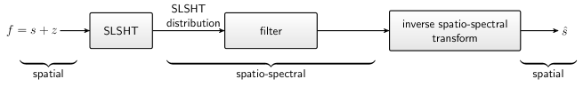
Figure 1: General schematic for spatio-spectral filtering. The spatial signal, $f=s+z$, on the 2-sphere, is first mapped to the spatio-spectral domain using the spatially localized spherical harmonic transform (SLSHT), then its SLSHT distribution is transformed in spatio-spectral domain, and the result is mapped back to the spatial domain using an inverse spatio-spectral transform to obtain the estimate $\tilde{s}$.

The rest of the paper is organized as follows. In Sections 2 and 3, the mathematical preliminaries and the spatio-spectral filtering framework are presented, respectively. The problem is formalized in Section 4 and the proposed optimal filter is derived in Section 5. In Section 6, an example of optimal estimation of a signal in noise, where both are described by anisotropic processes, is given. Finally, the concluding remarks and future directions are given in Section 7.

2 Mathematical Background

In this section, we briefly review some mathematical background for signals defined on the 2-sphere or unit sphere.

2.1 Signals on the 2-sphere

In this work, we consider the square integrable complex functions defined on the 2-sphere denoted by $\mathbb{S}^{2}$. Let $\boldsymbol{\hat{x}}\equiv\boldsymbol{\hat{x}}(\theta,\phi)\coloneqq(\sin\theta\cos\phi,\,\sin\theta\sin\phi,\,\cos\theta)^{\prime}\in\mathbb{R}^{3}$ and $\boldsymbol{\hat{y}}\equiv\boldsymbol{\hat{y}}(\vartheta,\varphi)\coloneqq(\sin\vartheta\cos\varphi,\,\sin\vartheta\sin\varphi,\,\cos\vartheta)^{\prime}\in\mathbb{S}^{2}$ denote unit vectors, where ^′ denotes the transpose, Each of the unit vectors parameterizes a point on the 2-sphere, with $\theta,\,\vartheta\in[0,\pi]$ denoting the co-latitude and $\phi,\,\varphi\in[0,2\pi)$ denoting the longitude.

The inner product of two functions $f(\boldsymbol{\hat{x}})$ and $h(\boldsymbol{\hat{x}})$ on $\mathbb{S}^{2}$ is defined as [13]

$$\big{\langle}f,h\big{\rangle}\coloneqq\int_{\mathbb{S}^{2}}f(\boldsymbol{\hat{x}})\,\overline{h(\boldsymbol{\hat{x}})}\,ds(\boldsymbol{\hat{x}}),$$ (1)

where $ds(\boldsymbol{\hat{x}})=\sin\theta\,d\theta\,d\phi$ is the area element, $\overline{(\cdot)}$ denotes complex conjugate and the integration is carried out over the whole sphere. With the inner product in (1), the space of square integrable complex valued functions on the sphere forms a complete Hilbert space $L^{2}(\mathbb{S}^{2})$. Also, the inner product in (1) induces a norm $\lVert f\rVert\coloneqq\langle f,f\rangle{}^{1/2}$. We refer to the functions with finite induced norm as signals on the 2-sphere.

2.2 Spectral Representation and Spherical Harmonics

The Hilbert space $L^{2}(\mathbb{S}^{2})$ is separable and spherical harmonic functions (or spherical harmonics for short) $Y_{\ell}^{m}(\boldsymbol{\hat{x}})=Y_{\ell}^{m}(\theta,\phi)$ [13, 20] of all integer degrees $\ell\geq 0$ and integer orders $-\ell\leq m\leq\ell$ form the archetype complete orthonormal set of basis functions. By completeness, any signal $f\in L^{2}(\mathbb{S}^{2})$ can be expanded as

$$f(\boldsymbol{\hat{x}})=\sum_{{\ell}=0}^{\infty}\sum_{m=-{\ell}}^{\ell}({f})_{\ell}^{m}Y_{\ell}^{m}(\boldsymbol{\hat{x}}),\quad({f})_{\ell}^{m}\coloneqq\big{\langle}f,Y_{{\ell}}^{m}\big{\rangle}=\int_{\mathbb{S}^{2}}f(\boldsymbol{\hat{x}})\overline{Y_{\ell}^{m}(\boldsymbol{\hat{x}})}\,ds(\boldsymbol{\hat{x}}),$$ (2)

where $({f})_{\ell}^{m}$ is the spherical harmonic coefficient of degree $\ell$ and order $m$, which forms part of the spectral domain representation of a signal and, therefore, is also referred as spectral component. The mathematical definition for the spherical harmonics is provided in Appendix A.1. The signal $f(\boldsymbol{\hat{x}})$ is said to be band-limited with maximum spectral degree $L_{f}$ if $({f})_{\ell}^{m}=0,\,\forall\ell>L_{f}$. For azimuthally symmetric function, where $h(\boldsymbol{\hat{x}})=h(\theta,\phi)=h(\theta)$, we note that only zero-order spherical harmonic coefficients of $h(\boldsymbol{\hat{x}})$ are non-zero, that is, $({h})_{\ell}^{m}=0$ for all $m\neq 0$.

For notational compactness, we express the spherical harmonic $Y_{\ell}^{m}$ as $Y_{n}$ and spherical harmonic coefficient $({f})_{\ell}^{m}$ as $({f})_{n}$. That is, as a function of a single integer index $n$ instead of two integer indices ${\ell}$ and $m$, using the one-to-one mapping

$$({\ell},m)\leftrightarrow n,\quad n={\ell}^{2}+{\ell}+m,\quad\ell=\lfloor\sqrt{n}\rfloor,\quad m=n-\lfloor\sqrt{n}\rfloor(\lfloor\sqrt{n}\rfloor-1),$$ (3)

where $\lfloor\,\cdot\,\rfloor$ denotes the integer floor function. Using this mapping, the spectral response can be denoted by $\boldsymbol{f}=\big{(}({f})_{0},\,({f})_{1},\,({f})_{2},\,\dotsc\big{)}^{\prime}$. If $f(\boldsymbol{\hat{x}})$ is band-limited in degree to $L_{f}$, then $\boldsymbol{f}=\big{(}({f})_{0},({f})_{1},({f})_{2},\dotsc,({f})_{N_{f}}\big{)}^{\prime}$, where $N_{f}=L_{f}^{2}+2L_{f}$.

2.3 Rotations on the Sphere

Here, we only define the rotation for azimuthally symmetric signals on the 2-sphere. We refer the reader elsewhere [13] for comprehensive details for rotations defined on the 2-sphere. Define the rotation operator $\mathcal{D}(\boldsymbol{\hat{y}})$ with $\boldsymbol{\hat{y}}=\boldsymbol{\hat{y}}(\vartheta,\varphi)$, which rotates the azimuthally symmetric functions $h(\boldsymbol{\hat{x}})$ by $\vartheta\in[0,\,\pi]$ about $y-$axis followed by a $\varphi\in[0,\,2\pi)$ rotation about $z-$axis. Under this rotation operation $\mathcal{D}(\boldsymbol{\hat{y}})$, the spherical harmonic coefficients of the rotated signal are related to those of the original signal through [13]

$$\big{(}\mathcal{D}(\boldsymbol{\hat{y}})h\big{)}_{\ell}^{m}=\sqrt{\frac{4\pi}{2\ell+1}}\overline{Y_{\ell}^{m}(\vartheta,\varphi)}({h})_{\ell}^{0},\quad\boldsymbol{\hat{y}}=\boldsymbol{\hat{y}}(\vartheta,\varphi).$$ (4)

2.4 Convolution

There are different definitions of spherical convolution available in the literature [21, 22, 23]. In this paper, we follow the definition of convolution presented as harmonic multiplication [22]

$$\big{(}h\circledast f\big{)}(\boldsymbol{\hat{y}})\coloneqq\sum_{{\ell}=0}^{\infty}\sum_{m=-\ell}^{\ell}({h})_{\ell}^{m}({f})_{\ell}^{m}Y_{\ell}^{m}(\boldsymbol{\hat{y}}),$$ (5)

where $({h})_{\ell}^{m}=\big{\langle}h,Y_{{\ell}}^{m}\big{\rangle}$ and $({f})_{\ell}^{m}=\big{\langle}f,Y_{{\ell}}^{m}\big{\rangle}$. We also note that

$$({h\circledast f})_{\ell}^{m}=\big{\langle}h\circledast f,Y_{{\ell}}^{m}\big{\rangle}=({h})_{\ell}^{m}({f})_{\ell}^{m}.$$ (6)

2.5 Stochastic Processes on the Sphere

Let $z(\boldsymbol{\hat{x}})$ denotes a realization of a zero-mean, Gaussian, anisotropic, random process on the 2-sphere with spectral domain representation

$$z(\boldsymbol{\hat{x}})=\sum_{n}^{\infty}({z})_{n}Y_{n}(\boldsymbol{\hat{x}}).$$ (7)

Since we assume the process to be zero-mean and Gaussian, we take $({z})_{n}$ to be complex-valued jointly normal random variables and therefore the covariance between the spherical harmonic coefficients completely characterizes the process. Define $\mathbf{C}_{Z}$ as the spectral covariance matrix with entries of the form $\mathbf{C}_{Z}^{nr}$ given by

$$\mathbf{C}_{Z}^{nr}\coloneqq\operatorname{\mathbb{E}}\big{\{}({z})_{n}\overline{({z})_{r}}\big{\}}$$ (8)

as a measure of the covariance between spectral coefficients $({z})_{n}$ and $({z})_{r}$ of the realizations of the processes, where $\operatorname{\mathbb{E}}\{\cdot\}$ denotes the expectation operator. Also, define the spatial covariance function $C_{Z}(\boldsymbol{\hat{x}},\boldsymbol{\hat{y}})=\operatorname{\mathbb{E}}\{z(\boldsymbol{\hat{x}})\overline{z(\boldsymbol{\hat{y}})}\}$ which relates the process values at two spatial positions. Given the spectral covariance matrix $\mathbf{C}_{Z}$, the spatial covariance $C_{Z}(\boldsymbol{\hat{x}},\boldsymbol{\hat{y}})$ can be determined as

$$C_{Z}(\boldsymbol{\hat{x}},\boldsymbol{\hat{y}})=\sum_{n=0}^{\infty}\sum_{r=0}^{\infty}\mathbf{C}_{Z}^{nr}Y_{n}(\boldsymbol{\hat{x}})\overline{Y_{r}(\boldsymbol{\hat{y}})}$$ (9)

We note that the covariance matrix $\mathbf{C}_{Z}$, or the covariance function $C_{Z}(\boldsymbol{\hat{x}},\boldsymbol{\hat{y}})$, given in (8), or (9), is the most general characterization of the random Gaussian (anisotropic) process on the sphere [24], which can be used to describe some special processes on the 2-sphere. For example, spectral covariance matrices for isotropic process and azimuthally symmetric process are given by

Isotropic process: $$\quad\mathbf{C}_{Z}^{nr}=C_{\ell}\delta_{nr},\quad(\ell,m)\leftrightarrow n,$$

Azimuthally-symmetric process: $$\quad\mathbf{C}_{Z}^{nr}=C^{m}_{\ell p}\delta_{mq},\quad(\ell,m)\leftrightarrow n,\,(p,q)\leftrightarrow r,$$

for some real $C_{\ell}$ and $C^{m}_{\ell p}$ which can be used in conjunction with (9) to determine spatial covariance functions as

Isotropic process: $$\quad C_{Z}(\boldsymbol{\hat{x}},\boldsymbol{\hat{y}})=\sum_{\ell=0}^{\infty}\frac{2\ell+1}{4\pi}C_{\ell}P_{\ell}^{0}(\boldsymbol{\hat{x}}\cdot\boldsymbol{\hat{y}}),$$

Azimuthally-symmetric process: $$\quad C_{Z}(\boldsymbol{\hat{x}},\boldsymbol{\hat{y}})=\sum_{m={-\infty}}^{\infty}\,\sum_{\ell=|m|}^{\infty}\,\sum_{p=|m|}^{\infty}C^{m}_{\ell p}\,N_{\ell}^{m}N_{p}^{m}\,P_{\ell}^{m}(\cos\theta)P_{p}^{m}(\cos\theta).$$

3 Spatio-Spectral Filtering Framework

In this paper, we are interested in the filtering and modification of signals in the joint spatio-spectral domain. We use the spatially localized spherical harmonic transform (SLSHT) distribution as a representation of signal in the spatio-spectral domain [19, 15, 25]. The SLSHT distribution is obtained using spatially localized spherical harmonic transform (SLSHT) for signals on the 2-sphere, which is analogous to the short-time Fourier transform (STFT). We consider the filtering framework [15] shown in Fig. 1, where the SLSHT distribution of the input signal is first obtained, then the SLSHT distribution is processed in the joint spatio-spectral domain to yield the filtered distribution and transformed back to the spatial domain using the SLSHT inverse operation.

Spatially Localized Spherical Harmonics Transform (SLSHT) Distribution

Analogous to the STFT, the SLSHT can be defined as a set of windowed spherical harmonic transforms [2, 19] to represent the signal jointly in the spatio-spectral domain. Mathematically, the SLSHT of the signal $f(\boldsymbol{\hat{x}})$ using an azimuthally symmetric window function $h(\boldsymbol{\hat{x}})$, evaluated at point $\boldsymbol{\hat{y}}=\boldsymbol{\hat{y}}(\vartheta,\varphi)$, degree $\ell$ and order $m$, is defined as

$$g_{f}(\boldsymbol{\hat{y}};{\ell},m)\equiv g_{f}(\boldsymbol{\hat{y}};n)\coloneqq\int_{\mathbb{S}^{2}}\big{(}\mathcal{D}(\boldsymbol{\hat{y}})h\big{)}(\boldsymbol{\hat{x}})f(\boldsymbol{\hat{x}})\overline{Y_{\ell}^{m}(\boldsymbol{\hat{x}})}\,ds(\boldsymbol{\hat{x}}),\quad(\ell,m)\leftrightarrow n.$$ (10)

which forms the SLSHT distribution given by

$$\boldsymbol{g}_{f}(\boldsymbol{\hat{y}})\coloneqq\big{(}g_{f}(\boldsymbol{\hat{y}};0),\,g_{f}(\boldsymbol{\hat{y}};1),\,g_{f}(\boldsymbol{\hat{y}};2),\,\dotsc\big{)}^{\prime},$$ (11)

as a representation of signal in the spatio-spectral domain. Unlike the spherical harmonic coefficient $({f})_{\ell}^{m}$, which is only a function of degree $\ell$ and order $m$, the SLSHT provides a spatially-varying spherical harmonic representation of the signal, that is, $g_{f}(\boldsymbol{\hat{y}};{\ell},m)$ is a function of the spatial localization $\boldsymbol{\hat{y}}$, degree $\ell$ and order $m$.

Remark 1

For mathematical simplification, we assume that the azimuthally symmetric window function $h(\boldsymbol{\hat{x}})$ is band-limited with maximum spectral degree $L_{h}$ and the spectral response is $\boldsymbol{h}=\big{(}({h})_{0},\,({h})_{1},\,({h})_{2},\dotsc,({h})_{N_{h}}\big{)}^{\prime}$, where $N_{h}=L_{h}^{2}+2L_{h}$. We further assume that the window function is unit energy normalized, that is, $\big{\langle}h,h\big{\rangle}=1$.

Summarizing the mathematical formulations developed elsewhere [19, 15], we express the SLSHT distribution component ${g}_{f}(\boldsymbol{\hat{y}};n)$ as

$${g}_{f}(\boldsymbol{\hat{y}};n) =\sum_{r=0}^{N_{h}}\Big{(}\sum_{c=0}^{\infty}({f})_{c}\sqrt{\frac{4\pi}{2p+1}}({h})_{p}^{0}\,T(c;r;n)\Big{)}\overline{Y_{p}^{q}(\boldsymbol{\hat{y}})}$$

$$=\sum_{c=0}^{\infty}({f})_{c}\,\psi_{n,c}(\boldsymbol{\hat{y}}),$$ (12)

with

$$\psi_{n,c}(\boldsymbol{\hat{y}})=\sum_{r=0}^{N_{h}}\sqrt{\frac{4\pi}{2p+1}}\overline{Y_{p}^{q}(\boldsymbol{\hat{y}})}({h})_{p}^{0}\,T(c;r;n),\quad(p,q)\leftrightarrow r$$ (13)

where

$$T(c;r;n)=T(r;c;n)\coloneqq\int_{\mathbb{S}^{2}}Y_{r}(\boldsymbol{\hat{x}})Y_{c}(\boldsymbol{\hat{x}})\overline{Y_{n}(\boldsymbol{\hat{x}})}\,ds(\boldsymbol{\hat{x}})$$ (14)

denotes the spherical harmonic triple product and its explicit expression is provided in Appendix A.2.

Remark 2

Comparing (3) with (2), we note that each distribution component ${g}_{f}(\boldsymbol{\hat{y}};n)$ is band-limited with maximum spectral degree $L_{h}$ (band-limit of the window function).

Spatially Varying Filtering

The SLSHT distribution represents the spatially-varying spectral representation of a signal as a function of both spatial location $\boldsymbol{\hat{y}}$ and degree and order $\ell,m$, and therefore offers the opportunity to filter the signal in the joint spatio-spectral domain. For this purpose, we define set of functions as the filter function

$$\boldsymbol{\zeta}(\boldsymbol{\hat{y}})\coloneqq\big{(}\zeta(\boldsymbol{\hat{y}};0),\,\zeta(\boldsymbol{\hat{y}};1),\,\zeta(\boldsymbol{\hat{y}};2),\,\dotsc\big{)}^{\prime}$$

in the spatio-spectral domain, with each element $\zeta(\boldsymbol{\hat{x}};n)$ for $0\leq n$ be a finite-norm, square integrable band-limited function on the 2-sphere with the maximum spectral degree $L_{\zeta_{n}}$ and spherical harmonic expansion $\zeta(\boldsymbol{\hat{y}};n)=\sum_{r=0}^{N_{\zeta_{n}}}({\zeta_{n}})_{r}Y_{r}(\boldsymbol{\hat{y}})$, where $N_{\zeta_{n}}=L_{\zeta_{n}}^{2}+2L_{\zeta_{n}}$.

Define the filtered distribution

$$\boldsymbol{v}(\boldsymbol{\hat{y}})\coloneqq\big{(}v(\boldsymbol{\hat{y}};0),\,v(\boldsymbol{\hat{y}};1),\,v(\boldsymbol{\hat{y}};2),\,\dotsc\big{)}^{\prime},$$

where each filtered distribution component ${v}(\boldsymbol{\hat{y}};n)$ is obtained as a convolution of the SLSHT component distribution $g_{f}(\boldsymbol{\hat{y}};n)$ and the corresponding element $\zeta(\boldsymbol{\hat{y}};n)$ of the filter function $\boldsymbol{\zeta}(\boldsymbol{\hat{y}})$, that is,

$${v}(\boldsymbol{\hat{y}};n)=\big{(}g_{f}(\cdot\,;n)\circledast\zeta(\cdot\,;n)\big{)}(\boldsymbol{\hat{y}}).$$ (15)

By defining

$$G_{f}(r;n)=\big{\langle}g_{f}(\cdot\,;n),Y_{r}\big{\rangle}$$

and using the formulation of convolution given in (5), we express the filtered distribution component ${v}(\boldsymbol{\hat{y}};n)$ in (15) as

$${v}(\boldsymbol{\hat{y}};n)=\smashoperator[]{\sum_{r=0}^{\min(N_{h},N_{\zeta_{n}})}}G_{f}(r;n)({\zeta_{n}})_{r}Y_{r}(\boldsymbol{\hat{y}}).$$ (16)

Remark 3

Following Remark 2 and noting the fact that each component ${v}(\boldsymbol{\hat{y}};n)$ of the filtered distribution is obtained as a result of convolution of $g_{f}(\boldsymbol{\hat{y}};n)$ and $\zeta(\boldsymbol{\hat{y}};n)$, which corresponds to the multiplication in the spectral domain as described in (6), the summation in (16) is truncated at the minimum of $N_{h}$ and $N_{\zeta_{n}}$. For simplicity, we assume that each filter component $\zeta(\boldsymbol{\hat{y}};n)$ is band-limited with maximum spectral degree $L_{h}$, that is, $L_{\zeta_{n}}=L_{h}$ for $n\in\{1,2,\dotsc\}$.

Inverse SLSHT

Here we present inverse SLSHT to obtain the signal $\tilde{s}(\boldsymbol{\hat{x}})\in L^{2}(\mathbb{S}^{2})$ having spectral response $\boldsymbol{s}$ and the SLSHT distribution $\boldsymbol{g}_{\tilde{s}}(\boldsymbol{\hat{y}})$, which approximates $\boldsymbol{v}(\boldsymbol{\hat{y}})$ in the least squares sense. We can determine such a signal $\tilde{s}(\boldsymbol{\hat{x}})$ in spectral domain as [15]

$$({\tilde{s}})_{c}=\sum_{n=0}^{\infty}\int_{\mathbb{S}^{2}}\overline{\psi_{c,n}}(\boldsymbol{\hat{y}})\,{v}(\boldsymbol{\hat{y}};n)\,ds(\boldsymbol{\hat{y}}).$$ (17)

4 Problem Formulation

With all of the necessary mathematical background presented, we formulate the problem under consideration, namely the estimation of signals on the 2-sphere from noisy observations. We consider the complex valued signals on the 2-sphere, contaminated by anisotropic additive noise for which the statistical properties are only known. Assume that the signal of interest is $s(\boldsymbol{\hat{x}})$, contaminated by additive noise $z(\boldsymbol{\hat{x}})$. Given

$$f(\boldsymbol{\hat{x}})=s(\boldsymbol{\hat{x}})+z(\boldsymbol{\hat{x}}),$$ (18)

we consider the problem to find the optimal (in a sense to be defined) estimate of the signal $s(\boldsymbol{\hat{x}})$.

The noise is considered to be a realization of zero mean, Gaussian, anisotropic, random process on the 2-sphere with known covariance matrix $\mathbf{C}_{Z}$. We also assume that the signal of interest $s(\boldsymbol{\hat{x}})$, itself, may be a realization of zero mean, Gaussian, anisotropic, random process for which the covariance matrix $\mathbf{C}_{S}$ is also known. Furthermore, we assume that noise and signal are uncorrelated, that is, $\operatorname{\mathbb{E}}\{s(\boldsymbol{\hat{x}})\overline{z(\boldsymbol{\hat{x}}})\}=0$ (or equivalently $\operatorname{\mathbb{E}}\{({s})_{n}\overline{({z})_{r}}\}=0$). We note that the problem under consideration, which is to estimate the signal $s(\boldsymbol{\hat{x}})$ from $f(\boldsymbol{\hat{x}})$, is equivalent to finding the best estimate $({\tilde{s}})_{n}$ of the spherical harmonic expansion coefficients $({s})_{n}$ forming the spectral response, $\boldsymbol{s}$ of the signal $s(\boldsymbol{\hat{x}})$.

We also need to clarify what we understand by “optimal” in this context; we seek an estimate $\tilde{s}(\boldsymbol{\hat{x}})$ (or $\boldsymbol{\tilde{s}}$), which minimizes the mean-square error (MSE) between the estimate and the desired signal. Define the MSE $\mathcal{E}_{s}$, that is, the expected energy of the estimation error as

$$\mathcal{E}_{s} =\operatorname{\mathbb{E}}\Big{\{}\big{\lVert}s(\boldsymbol{\hat{x}})-\tilde{s}(\boldsymbol{\hat{x}})\big{\rVert}^{2}\Big{\}}$$

$$=\operatorname{\mathbb{E}}\big{\{}(\boldsymbol{s}-\boldsymbol{\tilde{s}})^{H}(\boldsymbol{s}-\boldsymbol{\tilde{s}})\big{\}},$$ (19)

where $(\cdot)^{H}$ denotes the Hermitian and the second equality which quantifies the error between the estimate and the signal in the spectral domain, follows from the orthonormality of spherical harmonics.

For isotropic processes, there exist simple spectral domain formulations for optimal filters which minimizes the mean-square error between the estimate and the signal [11] or equivalently the variance of the unbiased estimate [10]. In our present formulation the signal and noise processes can be anisotropic, and this puts us in the realm of designing spatially-varying optimal filters for the estimation of a signal from its noise contaminated version. We design such an optimal filter in the next section.

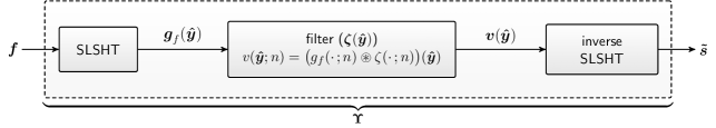
Figure 2: The spatio-spectral filtering framework: $\boldsymbol{f}$ is the spectral response of the signal $f(\boldsymbol{\hat{x}})$ on the 2-sphere, $\boldsymbol{g}_{f}(\boldsymbol{\hat{y}})$ is corresponding SLSHT distribution in the spatio-spectral domain, which convolves with the filter function $\boldsymbol{\zeta}(\boldsymbol{\hat{y}})$ to generate filtered distribution $\boldsymbol{v}(\boldsymbol{\hat{y}})$ and $\boldsymbol{\tilde{s}}$ is the spectral response of the estimated signal $\tilde{s}(\boldsymbol{\hat{x}})$, obtained using inverse SLSHT. The transformation between the spectral responses is linear and given by the spatio-spectral transformation matrix $\boldsymbol{\Upsilon}$.

5 Optimal Filtering in Spatio-Spectral Domain

We consider the spatio-spectral filtering framework presented in Section 3 to estimate the signal $s(\boldsymbol{\hat{x}})$ from $f(\boldsymbol{\hat{x}})$. As depicted in Fig. 2, let $f(\boldsymbol{\hat{x}})$, given in (18), be the input signal to the filtering framework, where the filter function $\boldsymbol{\zeta}(\boldsymbol{\hat{y}})$ convolves with the SLSHT distribution $\boldsymbol{g}_{f}(\boldsymbol{\hat{y}})$ of the input signal $f(\boldsymbol{\hat{x}})$, generating a filtered distribution $\boldsymbol{v}(\boldsymbol{\hat{y}})$ for which we obtain the signal estimate $\tilde{s}(\boldsymbol{\hat{x}})$ using inverse SLSHT. In this setting, the estimation problem formulated in the previous section reduces to determine such an optimal filter $\boldsymbol{\zeta}(\boldsymbol{\hat{y}})$ that minimizes the mean square error, given in (4), between the signal estimate ${\tilde{s}(\boldsymbol{\hat{x}})}$ and the uncontaminated signal signal $s(\boldsymbol{\hat{x}})$. This is equivalent to seeking an optimal filter which minimizes the MSE between the filtered distribution $\boldsymbol{v}(\boldsymbol{\hat{x}})$ and the SLSHT distribution $\boldsymbol{g}_{s}(\boldsymbol{\hat{y}})$ of the uncontaminated signal $s(\boldsymbol{\hat{x}})$. Define the spatio-spectral MSE $\mathcal{E}_{ss}$ as

$${\mathcal{E}_{ss}} =\operatorname{\mathbb{E}}\big{\{}\sum_{n=0}^{\infty}\big{\lVert}{v}(\boldsymbol{\hat{y}};n)-{g}_{s}(\boldsymbol{\hat{y}};n)\big{\rVert}^{2}\big{\}}$$

$$=\operatorname{\mathbb{E}}\big{\{}\sum_{n=0}^{\infty}\big{\lVert}\big{(}g_{f}(\cdot\,;n)\circledast\zeta(\cdot\,;n)\big{)}(\boldsymbol{\hat{y}})-{g}_{s}(\boldsymbol{\hat{y}};n)\big{\rVert}^{2}\big{\}}.$$ (20)

Now we derive an optimal filter $\boldsymbol{\zeta}(\boldsymbol{\hat{y}})$ which minimizes MSE ${\mathcal{E}_{ss}}$ given in (5) and present the result in the form of following theorem.

Theorem 5.1 (Optimal filter in the spatio-spectral domain).

Let $f(\boldsymbol{\hat{x}})=s(\boldsymbol{\hat{x}})+z(\boldsymbol{\hat{x}})$ be the sum of a desired signal $s(\boldsymbol{\hat{x}})$ and a noise $z(\boldsymbol{\hat{x}})$. Further, let $\mathbf{C}_{S}$ and $\mathbf{C}_{Z}$ be the covariance matrices as defined in (8) for signal and noise processes, respectively. For $f(\boldsymbol{\hat{x}})$ as an input to the spatio-spectral filtering framework presented in Section 3 (shown in Fig. 2) with filter function $\boldsymbol{\zeta}(\boldsymbol{\hat{y}})=\big{(}\zeta(\boldsymbol{\hat{y}};0),\,\zeta(\boldsymbol{\hat{y}};1),\,\zeta(\boldsymbol{\hat{y}};2),\,\dotsc\big{)}^{\prime}$, the spectral response, $({\zeta_{n}})_{r}=\big{\langle}\zeta(\cdot\,;n),Y_{r}\big{\rangle}$ with $0\leq r\leq(N_{h}=L_{h}^{2}+2L_{h})$, of the optimal filter which minimizes the mean-square error ${\mathcal{E}_{ss}}$, formulated in (5), between the filtered distribution $\boldsymbol{v}(\boldsymbol{\hat{y}})$ and the SLSHT distribution $\boldsymbol{g}_{s}(\boldsymbol{\hat{y}})$, is given by

$$({\zeta_{n}})_{r}=\frac{\sum\limits_{c=0}^{\infty}\sum\limits_{c^{\prime}=0}^{\infty}H(c;r;n)H(c^{\prime};r;n)\mathbf{C}_{S}^{cc^{\prime}}}{\sum\limits_{c=0}^{\infty}\sum\limits_{c^{\prime}=0}^{\infty}H(c;r;n)H(c^{\prime};r;n)(\mathbf{C}_{S}^{cc^{\prime}}+\mathbf{C}_{Z}^{cc^{\prime}})}$$ (21)

for $n$ and $r$ such that $\sum\limits_{c=0}^{\infty}\sum\limits_{c^{\prime}=0}^{\infty}H(c;r;n)H(c^{\prime};r;n)(\mathbf{C}_{S}^{cc^{\prime}}+\mathbf{C}_{Z}^{cc^{\prime}})>0$ and is zero otherwise. Here $H(c;r;n)$ is given by

$$H(c;r;n)=(-1)^{q}\sqrt{\frac{4\pi}{2p+1}}({h})_{p}^{0}\,T(c;p,-q;n),\quad(p,q)\leftrightarrow r.$$

Proof: We first define

$$G_{s}(r;n)=\big{\langle}g_{s}(\cdot\,;n),Y_{r}\big{\rangle},\quad V(r;n)=\big{\langle}v(\cdot\,;n),Y_{r}\big{\rangle},$$

where $0\leq r\leq(N_{h}=L^{2}+2L_{h})$, following Remark 2 and

$$H(c;r;n)=\big{\langle}\psi_{n,c}(\cdot\,),Y_{r}\big{\rangle},$$ (22)

following (13). We can express $G_{f}(r;n)$ and $G_{s}(r;n)$ using the formulation of ${g_{f}(\boldsymbol{\hat{y}};n)}$ given in (3) and (22) as

$$G_{f}(r;n) =\sum_{c=0}^{\infty}({f})_{c}H(c;r;n)=\sum_{c=0}^{\infty}\left(({s})_{c}+({z})_{c}\right)H(c;r;n),$$

$$G_{s}(r;n) =\sum_{c=0}^{\infty}({f})_{c}H(c;r;n)=\sum_{c=0}^{\infty}({s})_{c}H(c;r;n),$$

and noting the effect of convolution in the spectral domain given in (6), $V(r;n)$ can be written as

$$V(r;n) =G_{f}(r;n)({\zeta_{n}})_{r}.$$ (23)

Using these formulations, we write the MSE ${\mathcal{E}_{ss}}$ in (5) as

$${\mathcal{E}_{ss}} =\operatorname{\mathbb{E}}\bigg{\{}\sum_{n=0}^{\infty}\big{\lVert}\sum_{r=0}^{N_{h}}\left(V(r;n)-G_{s}(r;n)\right)Y_{r}(\boldsymbol{\hat{y}})\big{\rVert}^{2}\bigg{\}}$$

$$=\sum_{n=0}^{\infty}\sum_{r=0}^{N_{h}}\operatorname{\mathbb{E}}\Big{\{}\big{\lvert}V(r;n)-G_{s}(r;n)\big{\rvert}^{2}\Big{\}}$$

$$=\sum_{n=0}^{\infty}\sum_{r=0}^{N_{h}}\sum_{c=0}^{\infty}\sum_{c^{\prime}=0}^{\infty}H(c;r;n)H(c^{\prime};r;n)$$

$$\qquad\times\operatorname{\mathbb{E}}\bigg{\{}\Big{(}({\zeta_{n}})_{r}\big{(}({s})_{c}+({z})_{c}\big{)}-({s})_{c}\big{)}\Big{(}\overline{({\zeta_{n}})_{r}}\big{(}\overline{({s})_{c^{\prime}}}+\overline{({z})_{c^{\prime}}}\big{)}-\overline{({s})_{c^{\prime}}}\big{)}\bigg{\}}.$$ (24)

Here $\big{\lvert}(\cdot)\big{\rvert}^{2}\coloneqq(\cdot)\overline{(\cdot)}$. Now, noting the fact that the signal and noise are uncorrelated, that is $\operatorname{\mathbb{E}}\{({s})_{c}\overline{({z})_{c^{\prime}}}\}=0$ for all $c,\,c^{\prime}$, using $\operatorname{\mathbb{E}}\{({s})_{c}\overline{({s})_{c^{\prime}}}\}=\mathbf{C}_{S}^{cc^{\prime}}$ and $\operatorname{\mathbb{E}}\{({z})_{c}\overline{({z})_{c^{\prime}}}\}=\mathbf{C}_{Z}^{cc^{\prime}}$ and setting the derivative of MSE ${\mathcal{E}_{ss}}$ in (5), with respect to $\overline{({\zeta_{n}})_{r}}$, equal to zero, we obtain the result stated in (21) for spectral response of the optimal filter $\boldsymbol{\zeta}(\boldsymbol{\hat{y}})$.

∎

Remark 5.2.

For the case when signal distortions are less than acceptable, we might require an optimal filter which minimizes a weighted MSE. The weighted MSE is obtained by assigning weight $\alpha$ to the factor in the MSE given in (5) that is due to the noise, and assigning weight $(1-\alpha)$ to the remaining factor. This amounts to replacing $\mathbf{C}_{Z}$ by $\alpha\mathbf{C}_{Z}$ and $\mathbf{C}_{S}$ by $(1-\alpha)\mathbf{C}_{S}$ in the solution of the optimal filter in (21).

The optimal filter signal estimate $\tilde{s}(\boldsymbol{\hat{x}})$ can be recovered form the spectral domain signal $\boldsymbol{\tilde{s}}$ using the inverse SLSHT operation. Using (17), we obtain the estimate $({\tilde{s}})_{c}$ as

$$({\tilde{s}})_{c} =\sum_{n=0}^{\infty}\int_{\mathbb{S}^{2}}\overline{\psi_{c,n}}(\boldsymbol{\hat{y}})\,{v}(\boldsymbol{\hat{y}};n)\,ds(\boldsymbol{\hat{y}})$$

$$=\sum_{n=0}^{\infty}\sum_{c^{\prime}=0}^{\infty}\sum_{r=0}^{N_{h}}({f})_{c^{\prime}}({\zeta_{n}})_{r}\,H(c;r;n)\,H(c^{\prime};r;n).$$ (25)

By defining the matrix $\mathbf{\Upsilon}$ with entries

$$\mathbf{\Upsilon}^{c,c^{\prime}}=\sum_{n=0}^{\infty}\sum_{r=0}^{N_{h}}({\zeta_{n}})_{r}\,H(c;r;n)\,H(c^{\prime};r;n).$$ (26)

the overall process of finding the desired signal estimate $\tilde{s}(\boldsymbol{\hat{x}})$ with spectral response $\boldsymbol{\tilde{s}}$, from the signal $f(\boldsymbol{\hat{x}})$ with spectral response $\boldsymbol{f}$ can be expressed as following linear transformation as shown in Fig. 2, that is,

$$\boldsymbol{\tilde{s}}=\mathbf{\Upsilon}\boldsymbol{f}.$$ (27)

The optimal filter in the spatio-spectral domain, derived in Theorem 5.1, extends the spectral domain formulation of optimal isotropic symmetric filter [9], which is valid for isotropic processes, to the broader class of anisotropic processes. Since we have defined $G_{s}(r;n)=\big{\langle}g_{s}(\cdot\,;n),Y_{r}\big{\rangle}$, we note that the spatio-spectral domain can be parameterized by $n$ and $r$ (recalling $n,\,r\in\mathbb{Z}^{+})$. With this characterization of spatio-spectral domain at hand, the formulation of optimal filter in the spatio-spectral domain given in (21) has a simple and intuitively appealing interpretation. For the values of $n$ and $r$: 1) where only the contribution of signal is present, that is, $G_{z}(r;n)\approx 0$, the optimal filter is approximately one, thus allows the signal to pass through without distortion; 2) where only the noise contribution is present, that is, $G_{s}(r;n)\approx 0$, or contribution of both signal and noise are not present, that is, $G_{s}(r;n)\approx G_{z}(r;n)\approx 0$, the optimal filter is approximately zero and therefore it suppresses the noise; and 3) where the contribution of both noise and signal are present, the optimal filter performs a weighting that depends on the signal and noise contribution in the spatio-spectral domain at the respective values of $n$ and $r$.

Remark 5.3.

Since the SLSHT distribution as a spatio-spectral representation is obtained using a window function, the overall optimal filtering is dependent on the chosen window function, the choice of which entails a trade-off between its resolution in the spatial and spectral domains. In time-frequency analysis, the analogous problem is resolved by extending the use of multiple windows (a set of orthogonal windows), the concept originally introduced by Thompson [26], in obtaining the STFT representation for the filtering of non-stationary signal in the time-frequency domain [27]. The same multi-window concept is used for the estimation of power spectrum for signals on the 2-sphere from the observations available over some spatially limited region [3]. We anticipate that the similar concept can be employed to improve the performance of the proposed optimal filter. However, further exploration in this direction is a subject of future work.

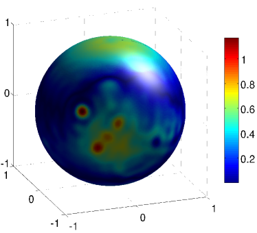
(a) Desired signal $s(\boldsymbol{\hat{x}})$

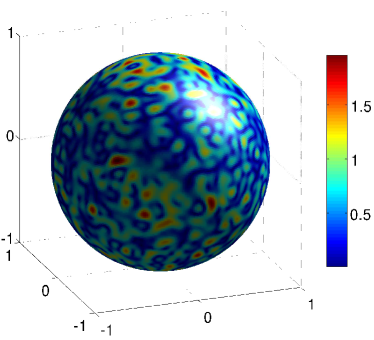
(b) Noise contaminated signal $f(\boldsymbol{\hat{x}})=s(\boldsymbol{\hat{x}})+z(\boldsymbol{\hat{x}})$

Figure 3: (a) The magnitude of the desired signal (Mars topographic map) $s(\boldsymbol{\hat{x}})$, band-limited with maximum spectral degree $L_{s}=36$ and (b) the magnitude of the noise contaminated signal $f(\boldsymbol{\hat{x}})=s(\boldsymbol{\hat{x}})+z(\boldsymbol{\hat{x}})$ with $\textrm{SNR}^{f}=-0.04$dB.

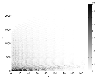
(a) ${\big{\lvert}G_{s}(r;n)\big{\rvert}}$

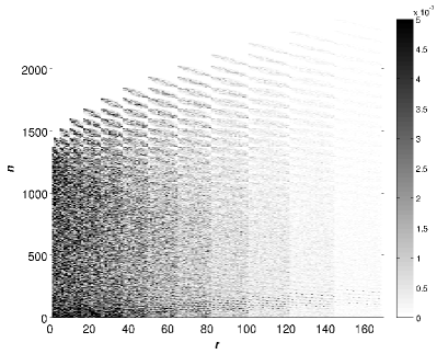
(b) ${\big{\lvert}G_{f}(r;n)\big{\rvert}}$

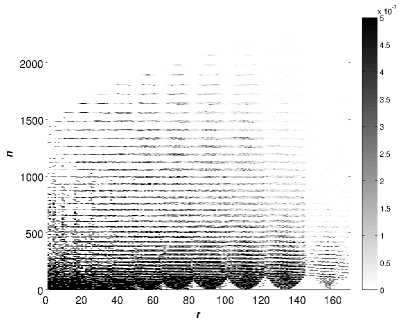
(c) ${\big{\lvert}({\zeta_{n}})_{r}\big{\rvert}}$

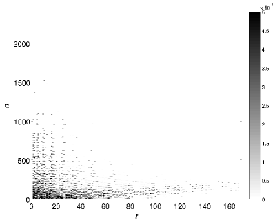
(d) ${\big{\lvert}V(r;n)\big{\rvert}}$

Figure 4: The SLSHT distributions $\boldsymbol{g}_{s}(\boldsymbol{\hat{y}})$ (for the desired signal) and $\boldsymbol{g}_{f}(\boldsymbol{\hat{y}})$ (for the noise contaminated signal) are shown in (a) $\lvert G_{s}(r;n)\rvert$ and (b) $\lvert G_{f}(r;n)\rvert$. The optimal filter $\boldsymbol{\zeta}(\boldsymbol{\hat{y}})$ derived in the spectral domain using the result in Theorem 5.1 is shown as (c) $\lvert({\zeta_{n}})_{r}\rvert$ and (d) the filtered distribution $\boldsymbol{v}(\boldsymbol{\hat{y}})$ is shown as $\lvert V(r;n)\rvert$. All of the plots are shown for $0\leq r\leq N_{h}$ and $0\leq n\leq N_{g}$.

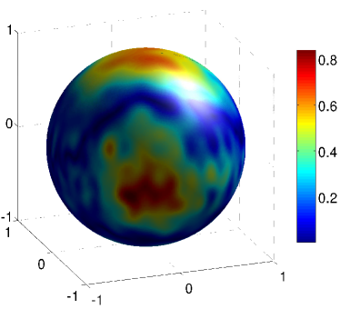
Figure 5: The magnitude of the estimated signal $\tilde{s}(\boldsymbol{\hat{x}})$, obtained from filtering the signal $f(\boldsymbol{\hat{x}})$ shown in Fig. 3(b) using the proposed optimal filter in the spatio-spectral domain. The SNR of the output signal is $\textrm{SNR}^{\tilde{s}}=24.7$dB.

6 Optimal Filter Design Example

We apply the proposed optimal filter in the spatio-spectral domain to enhance a signal that has been corrupted by anisotropic noise. The objective here is to demonstrate the performance of the proposed filter. We use signal-to-noise ratio (SNR) as a measure to quantify the performance of the optimal filter. If $s(\boldsymbol{\hat{x}})$ denotes the desired signal, we define the SNR for the signal $f(\boldsymbol{\hat{x}})$ as

$$\textrm{SNR}^{f}=20\log\frac{\big{\lVert}s(\boldsymbol{\hat{x}})\big{\rVert}}{\big{\lVert}f(\boldsymbol{\hat{x}})-s(\boldsymbol{\hat{x}})\big{\rVert}}.$$

in order to quantify the performance of the proposed optimal filter in the spatio-spectral domain. The implementation of optimal filtering framework is implemented in MATLAB, using the MATLAB interface of the SSHT package. The SLSHT distribution is computed using the efficient method proposed in literature[25].

We consider the Mars topographic map (height above geoid) as a desired signal $s(\boldsymbol{\hat{x}})$, which is synthesized using the spherical harmonic model of the topography of Mars. For convenience, the desired signal is made band-limited with band-limit $L_{s}=36$. We normalize the signal such that it has unit energy, that is, $\lVert s\rVert=1$. The desired signal $s(\boldsymbol{\hat{x}})$ is shown in Fig. 3(a). The noise is assumed to be a realization of zero mean, Gaussian, anisotropic, random process on the 2-sphere with known covariance matrix $\mathbf{C}_{Z}$. The covariance matrix is constructed as $\mathbf{C}_{Z}=\mathbf{A}\,\mathbf{A}^{H}$, where the entries of matrix $\mathbf{A}$ are complex with real and imaginary parts uniformly distributed in the interval $[0,1]$. The covariance matrix is then normalized such that the noise process has unit energy within the band-limit of the desired signal $L_{s}$, that is, $\sum_{n=0}^{L_{s}^{2}+2L_{s}}\mathbf{C}_{Z}^{rr}=1$. The noise $z(\boldsymbol{\hat{x}})$ is then generated in the spectral domain using the covariance matrix. It should be noted that the generated noise is complex valued.

The sum of the desired signal and the noise, that is, the noise contaminated signal $f(\boldsymbol{\hat{x}})=s(\boldsymbol{\hat{x}})+z(\boldsymbol{\hat{x}})$, is shown in Fig. 3(b). It is applied as an input to the spatio-spectral filtering framework shown in Fig. 2. The SLSHT distribution of the input signal is obtained using the azimuthally symmetric band-limited eigenfunction window [19] with band-limit $L_{h}=12$ and $99\%$ energy concentration in a polar cap region of central angle $\pi/6$. The SLSHT distributions $\boldsymbol{g}_{s}(\boldsymbol{\hat{y}})$ (desired) and $\boldsymbol{g}_{f}(\boldsymbol{\hat{y}})$ (input) are plotted as $G_{s}(r;n)$ and $G_{f}(r;n)$ in Fig. 4(a) and Fig. 4(b), respectively. Since both the desired signal and the window function are band-limited signals on the 2-sphere, both $G_{s}(r;n)$ and $G_{f}(r;n)$ are only defined for $0\leq r\leq N_{h}$ and $0\leq n\leq N_{g}$, where $N_{g}=(L_{f}+L_{h})^{2}+2(L_{f}+L_{h})$. The optimal filter $({\zeta_{n}})_{r}$, defined in Theorem 5.1, is shown in Fig. 4(c) for different values of $n$ and $r$. The optimal filter is applied to the SLSHT distribution $\boldsymbol{g}_{f}(\boldsymbol{\hat{y}};n)$ to yield the filtered distribution $\boldsymbol{v}(\boldsymbol{\hat{y}})$ shown in Fig. 4(d) as $V(r;n)$, which is then inverted, using (5), to obtain the estimated signal $\tilde{s}(\boldsymbol{\hat{x}})$ shown in Fig. 5.

Since both the desired signal and the noise process covariance matrix are normalized to contain unit energy within the band-limit $L_{s}$, then the expected SNR is $0$dB. For the realization in this example the actual input SNR is $\textrm{SNR}^{f}\approx-0.04$dB and the output SNR is $\textrm{SNR}^{\tilde{s}}=24.7$dB. We note that the proposed optimal filter, taking into account the signal and noise statistics, provides significant SNR improvement. We have provided example merely to demonstrate the capability of the proposed spatio-spectral optimal filtering framework. The more rigorous analysis of the performance of the filter and the application to real data such as Cosmological Microwave Background (CMB) maps [28] and Gravity Recovery and Climate Experiment (GRACE) gravity models are the subjects of future work.

7 Conclusions

We have developed an optimal filter for the estimation of signals on the 2-sphere corrupted by the noise, for the case when both the signal and noise are realizations of anisotropic processes on the sphere. The optimal filter is based on transformation in the spatio-spectral domain recently presented in the literature, and minimizes the mean-square error between the estimated signal and desired signal. The proposed optimal filter, unlike filters available in literature, takes into account the anisotropic properties of random processes on the 2-sphere. Finally, we provided an example to demonstrate the capability of proposed optimal filter. For future work we highlight two open problems: employing an analogy of the multiple window method [26] used in time frequency analysis [27] for the improvement of performance of the proposed optimal filter; and the application of the proposed optimal filter to the real data.

Appendix A Mathematical Background

A.1 Spherical Harmonics

The spherical harmonic function, $Y_{\ell}^{m}(\boldsymbol{\hat{x}})=Y_{\ell}^{m}(\theta,\phi)$, for degree ${\ell}\geq 0$ and order $|m|\leq{\ell}$ is defined as [20]

$$Y_{\ell}^{m}(\theta,\phi)=N_{\ell}^{m}P_{\ell}^{m}(\cos\theta)\,e^{im\phi},$$

where $N_{\ell}^{m}$ is the normalization factor given by

$$N_{\ell}^{m}\coloneqq\sqrt{\frac{2{\ell}+1}{4\pi}\frac{({\ell}-m)!}{({\ell}+m)!}},$$

such that $\big{\langle}Y_{\ell}^{m},Y_{p}^{q}\big{\rangle}=\delta_{\ell p}\delta_{mq}$, where $\delta_{mq}$ is the Kronecker delta function: $\delta_{mq}=1$ for $m=q$ and is zero otherwise. $P_{\ell}^{m}(x)$ is the associated Legendre function defined for degree $\ell$ and order $0\leq m\leq\ell$ as

$$P_{\ell}^{m}(x) =\frac{(-1)^{m}}{2^{\ell}{\ell}!}(1-x^{2})^{m/2}\frac{d^{{\ell}+m}}{dx^{{\ell}+m}}(x^{2}-1)^{\ell}$$

$$P_{\ell}^{-m}(x) ={(-1)^{m}}\frac{({\ell}-m)!}{({\ell}+m)!}P_{\ell}^{m}(x),$$

for $|x|\leq 1$.

A.2 Spherical Harmonics Triple Product

Using the Wigner-$3j$ symbols [20], the spherical harmonic triple product $T(u;r;n)$ can be written using the mappings $(a,b)\leftrightarrow c$, $(p,q)\leftrightarrow r$ and $(\ell,m)\leftrightarrow n$ as

$$T(c;r;n)=(-1)^{m}\,\sqrt{\frac{(2a+1)(2p+1)(2\ell+1)}{4\pi}}\,\begin{pmatrix}a&p&\ell\\ 0&0&0\end{pmatrix}\begin{pmatrix}a&p&\ell\\ b&q&-m\end{pmatrix}.$$

- [1] Chung, M. K., Worsley, K. J., Nacewicz, B. M., Dalton, K. M., and Davidson, R. J., “General multivariate linear modeling of surface shapes using SurfStat,” NeuroImage 53(2), 491–505 (2010).
- [2] Simons, M., Solomon, S. C., and Hager, B. H., “Localization of gravity and topography: constraints on the tectonics and mantle dynamics of Venus,” Geophys. J. Int. 131, 24–44 (Oct. 1997).
- [3] Wieczorek, M. A. and Simons, F. J., “Localized spectral analysis on the sphere,” Geophys. J. Int. 162, 655–675 (Sept. 2005).
- [4] Audet, P., “Directional wavelet analysis on the sphere: Application to gravity and topography of the terrestrial planets,” J. Geophys. Res. 116 (Feb. 2011).
- [5] McEwen, J. D., Vielva, P., Wiaux, Y., Barreiro, R. B., Cayón, L., Hobson, M. P., Lasenby, A. N., Martínez-González, E., and Sanz, J. L., “Cosmological applications of a wavelet analysis on the sphere,” J. Fourier Anal. Appl. 13, 495–510 (Aug. 2007).
- [6] Wiaux, Y., Jacques, L., and Vandergheynst, P., “Correspondence principle between spherical and Euclidean wavelets,” Astrophys. J. 632, 15–28 (Oct. 2005).
- [7] Ward, D. B., Kennedy, R. A., and Williamson, R. C., “Theory and design of broadband sensor arrays with frequency invariant far-field beam patterns,” J. Acoust. Soc. Am. 97, 1023–1034 (Feb. 1995).
- [8] Pollock, T. S., Abhayapala, T. D., and Kennedy, R. A., “Introducing space into MIMO capacity calculations,” J. Telecommun. Syst. 24, 415–436 (Oct. 2003).
- [9] Klees, R., Revtova, A., Gunter, B. C., Ditmar, P., Oudman, E., Winsemius, H. C., and Savenije, H. H. G., “The design of an optimal filter for monthly GRACE gravity models,” Geophys. J. Int. 175(2), 417–432 (2008).
- [10] McEwen, J. D., Hobson, M. P., and Lasenby, A. N., “Optimal filters on the sphere,” IEEE Trans. Signal Process. 56, 3813–3823 (Aug. 2008).
- [11] Wei, L. and Kennedy, R. A., “Zero-forcing and mmse filters design on the 2-sphere,” in [Proc. IEEE Int. Conf. Acoust., Speech, Signal Process., ICASSP’2011 ], 4360–4363 (2011).
- [12] McEwen, J. D. and Wiaux, Y., “A novel sampling theorem on the sphere,” IEEE Trans. Signal Process. 59, 5876–5887 (Dec. 2011).
- [13] Kennedy, R. A. and Sadeghi, P., [Hilbert Space Methods in Signal Processing ], Cambridge University Press, Cambridge, UK (Mar. 2013).
- [14] Arora, R. and Parthasarathy, H., “Optimal estimation and detection in homogeneous spaces,” IEEE Trans. Signal Process. 58, 2623–2635 (May 2010).
- [15] Khalid, Z., Sadeghi, P., Kennedy, R. A., and Durrani, S., “Spatially varying spectral filtering of signals on the unit sphere,” IEEE Trans. Signal Process. 61, 530–544 (Feb. 2013).
- [16] Kirchauer, H., Hlawatsch, F., and Kozek, W., “Time-frequency formulation and design of nonstationary wiener filters,” in [Proc. IEEE Int. Conf. Acoust., Speech, Signal Process., ICASSP’1995 ], 3, 1549–1552 (1995).
- [17] Mark, W. D., “Spectral analysis of the convolution and filtering of non-stationary stochastic processes,” J. Sound Vibr. 11, 19–63 (Jan. 1970).
- [18] Matz, G. and Hlawatsch, F., “Robust time-varying wiener filters: theory and time-frequency formulation,” in [Proc. IEEE-SP International Symposium on Time-Frequency and Time-Scale Analysis, 1998 ], 401–404 (1998).
- [19] Khalid, Z., Durrani, S., Sadeghi, P., and Kennedy, R. A., “Spatio-spectral analysis on the sphere using spatially localized spherical harmonics transform,” IEEE Trans. Signal Process. 60, 1487–1492 (Mar. 2012).
- [20] Sakurai, J. J., [Modern Quantum Mechanics ], Addison Wesley Publishing Company, Inc., Reading, MA, 2nd ed. (1994).
- [21] Yeo, B. T. T., Ou, W., and Golland, P., “On the construction of invertible filter banks on the 2-sphere,” IEEE Trans. Image Process. 17, 283–300 (Mar. 2008).
- [22] Kennedy, R. A., Lamahewa, T. A., and Wei, L., “On azimuthally symmetric 2-sphere convolution,” Digital Signal Processing 5, 660–666 (Sept. 2011).
- [23] Sadeghi, P., Kennedy, R. A., and Khalid, Z., “Commutative anisotropic convolution on the 2-sphere,” IEEE Trans. Signal Process. 60, 6697–6703 (Dec. 2012).
- [24] Hitczenko, M. and Stein, M. L., “Some theory for anisotropic processes on the sphere,” Statistical Methodology 9(1–2), 211 –227 (2012).
- [25] Khalid, Z., Kennedy, R. A., Durrani, S., Sadeghi, P., Wiaux, Y., and McEwen, J. D., “Fast directional spatially localized spherical harmonic transform,” IEEE Trans. Signal Process. 61(9), 2192–2203 (2013).
- [26] Thomson, D. J., “Spectrum estimation and harmonic analysis,” Proc. IEEE 70(9), 1055–1096 (1982).
- [27] Kozek, W., Feichtinger, H., and Scharinger, J., “Matched multiwindow methods for the estimation and filtering of nonstationary processes,” in [Proc. IEEE International Symposium on Circuits and Systems (ISCAS) ], 2, 509–512 (1996).
- [28] Planck Collaboration, “ESA Planck blue book,” Tech. Rep. ESA-SCI(2005)1, ESA (2005).