Local Average Consensus in Distributed Measurement of Spatial-Temporal Varying Parameters: 1D Case

Abstract

We study a new variant of consensus problems, termed ‘local average consensus’, in networks of agents. We consider the task of using sensor networks to perform distributed measurement of a parameter which has both spatial (in this paper 1D) and temporal variations. Our idea is to maintain potentially useful local information regarding spatial variation, as contrasted with reaching a single, global consensus, as well as to mitigate the effect of measurement errors. We employ two schemes for computation of local average consensus: exponential weighting and uniform finite window. In both schemes, we design local average consensus algorithms to address first the case where the measured parameter has spatial variation but is constant in time, and then the case where the measured parameter has both spatial and temporal variations. Our designed algorithms are distributed, in that information is exchanged only among neighbors. Moreover, we analyze both spatial and temporal frequency responses and noise propagation associated with the algorithms. The tradeoffs of using local consensus, as compared to standard global consensus, include higher memory requirement and degraded noise performance. Arbitrary updating weights and random spacing between sensors are analyzed in the proposed algorithms.

I Introduction

Consensus of multi-agent systems comes in many varieties (e.g. [1, 2, 3, 4, 5]), and in this paper, we focus on a particular variety, namely average consensus (e.g. [6, 7, 8, 9, 10]). This refers to an arrangement where each of a network of agents is associated with a value of a certain variable, and a process occurs which ends up with all agents learning the average value of the variable. Finding an average of a set of values is apparently conceptually trivial; what makes average consensus nontrivial is the fact that an imposed graphical structure limits the nature of the steps that can be part of the averaging algorithm, each agent only being allowed to exchange information with its neighbors, as defined by an overlaid graphical structure. Issues also arise of noise performance, transient performance, effect of time delay, agent/link loss, etc ([11, 12, 13, 14]).

Finding an average also throws away much information. In many situations, one might well envisage that a local average might be useful, retaining the characteristics of local information meanwhile mitigating the effect of measurement error. For instance, one thousand weather stations across a city, instead of giving a single air pollution reading, might validly be used to identify hotspots of pollution, i.e. localities with high pollution; thus, instead of a global average, a form of local averaging, still mitigating the effects of some noise, might be useful.

We term this variant ‘local (average) consensus’, and distinguish it from the normal sort of consensus, termed here by way of contrast ‘global (average) consensus’.

We consider two schemes for computation of local average consensus. One involves the use of exponential weights to reflect ‘closeness’ of the agents measured in both topological and geographical distance (viz. the further a neighbor is, the lesser its value will affect the agent’s computation of its ‘local average’). The other scheme employs a finite window to reduce computation burden; the bounds of the finite window will be case-dependent in applications. In both schemes, we design local consensus algorithms to address first the case where the measured variable has spatial variation but is constant in time, and then the case where the measured variable has both spatial and temporal variations. In this paper we consider spatial variation in 1D for simplicity. The designed local consensus algorithms are distributed, as their global consensus counterparts, in that information exchange is allowed only among neighbors. As we will see, these algorithms have higher memory requirement than that of a global consensus algorithm (the latter can be made memoryless).

We also seek to understand the properties of the designed local consensus algorithms. In particular, we analyze both spatial and temporal frequency responses and noise propagation associated with the algorithms. To obtain a fully analytical result we limit our study to a 1D sensor network, which can find its application in power line monitoring, canal/river monitoring, detection of border intrusions, structural monitoring of railways/bridges/pipelines, etc [15, 16, 17, 18, 19]. Moreover, we investigate two generalizations of the designed local consensus algorithms, one with arbitrary updating weights and the other with random spacing between sensors.

We note that [20] proposed a “consensus filter” which allows the nodes of sensor networks to track the average of their time-varying noisy measurements. This problem is called “dynamic average consensus”, which is later further studied in e.g. [21, 22], and also in [23, 24, 25] under a different name “coordinated average tracking”. These works, however, deal still with global average consensus, because all nodes are required to track the same time-varying average value. By contrast, our goal of local average consensus is to have each node track the time-varying average value only within its spatial neighborhood, thereby retaining characteristics of locally measured information.

The rest of the paper is organized as follows. Section II presents local average consensus algorithms for the case where the measured variable has spatial variation but is constant in time. Section III and Section IV investigate spatial frequency response and noise propagation of the designed algorithms. Section V studies arbitrary weights and random spacing in the proposed local averaging algorithms. Section VI presents local consensus algorithms for the case where the measured variable has both spatial and temporal variations. This allows the treatment of Section VII of the frequency response associated with time variations. Finally, Section VIII states our conclusions. An initial version of this paper has been submitted for IEEE Conference on Decision and Control 2013. This version differs from the conference predecessor through inclusion of proofs of results, development of material on the frequency response to time-variation in measured variables, and analysis of random spacing and arbitrary weights in the proposed algorithms.

II Distributed Local Consensus Algorithms

Consider a variable whose values vary in 1D space, and/or in addition vary in time. Suppose we have a (possibly infinite) chain of sensors to be placed (uniformly) along the 1D space. Each sensor $i$ has two variables: a measurement variable $x_{i}$ and a consensus variable $y_{i}$. At each time $k=0,1,2,...$ each sensor $i$ takes a measurement $x_{i}(k)$ (potentially noisy) of the variable. Our goal is to design distributed algorithms which update each sensor $i$’s consensus variable $y_{i}(k)$, based on $x_{i}(k)$ and information only from the two immediate neighbors $i-1$ and $i+1$, such that $y_{i}(k)$ converges to a value which reflects spatial-temporal variations of the variable (as we define below).

In this section, we focus on the case where all local measurements are time-invariant, i.e. $x_{i}(k)=x_{i}$ (a constant) for all $i,k$. The time-varying case will be addressed in Section VI, below. We consider two types of weighting schemes: exponential weighting and uniform finite window.

II-A Exponential Weighting

For computing a local average at sensor $i$, it is natural to assign larger weights to information that is spatially closer to $i$. One way of doing so is to assign an exponential weight $\rho^{j}$, $\rho\in(0,1)$ and $j$ a nonnegative integer, to a measurement taken at distance $j$ from $i$. For this scheme, we formulate the following problem, adopting the reasonable assumption that there is a bound $M<\infty$ such that measurement variables $|x_{i}|<M$ for all $i$.

Problem 1. Let $\rho\in(0,1)$. Design a distributed algorithm to update each sensor $i$’s consensus variable $y_{i}(k)$ such that

$$\lim_{k\rightarrow\infty}y_{i}(k)=\frac{1-\rho}{1+\rho}\left(x_{i}+\sum_{j=1}^{\infty}\rho^{j}(x_{i-j}+x_{i+j})\right).$$ (1)

Thus, exponentially decaying weights, at the rate $\rho$, are assigned to the information from both forward and backward directions. Note that the limit of $y_{i}(k)$ exists because all $x_{i}$ are assumed bounded. The scaling constant $(1-\rho)/(1+\rho)$ ensures that, if all $x_{i}$ are the same, $y_{i}(k)$ is in the limit equal to $x_{i}$.

We propose the following distributed algorithm to solve Problem 1. For all $i$,

$$y_{i}(0) =\frac{1-\rho}{1+\rho}x_{i}$$ (2a)

$$y_{i}(1) =y_{i}(0)+\rho(y_{i-1}(0)+y_{i+1}(0))$$ (2b)

$$y_{i}(2) =y_{i}(1)+\rho(y_{i-1}(1)-y_{i-1}(0))+$$ (2c)

$$\hskip 14.22636pt\rho(y_{i+1}(1)-y_{i+1}(0))-\rho^{2}2y_{i}(0)$$

$$y_{i}(k+1) =y_{i}(k)+\rho(y_{i-1}(k)-y_{i-1}(k-1))+$$ (2d)

$$\rho(y_{i+1}(k)-y_{i+1}(k-1))-\rho^{2}(y_{i}(k-1)-y_{i}(k-2)),\ k\geq 2.$$

Each sensor $i$ needs information only from its two immediate neighbors: $y_{i-1}(k)$ and $y_{i+1}(k)$, $k=0,1,...$. At each iteration $k\ (\geq 2)$, the quantities used to update $y_{i}(k)$ are $y_{i-1}(k)-y_{i-1}(k-1)$, $y_{i+1}(k)-y_{i+1}(k-1)$, and $y_{i}(k-1)-y_{i}(k-2)$. Thus more memory is required in this local consensus algorithm than in a global consensus algorithm, though the increase is obviously modest.

Theorem 1.

Algorithm (2) solves Problem 1.

Proof. We will show by induction on $k\geq 1$ that

$$y_{i}(k)=y_{i}(k-1)+\rho^{k}(y_{i-k}(0)+y_{i+k}(0)),\ \ \forall i.$$ (3)

This leads to

$$y_{i}(k) =y_{i}(0)+\sum_{j=1}^{k}\rho^{j}(y_{i-j}(0)+y_{i+j}(0))$$

$$=\frac{1-\rho}{1+\rho}\left(x_{i}+\sum_{j=1}^{k}\rho^{j}(x_{i-j}+x_{i+j})\right),\ \ \forall i.$$

The second equality above is due to (2a). Then taking the limit as $k\rightarrow\infty$ yields (1). That the limit exists follows from the fact that $|x_{i}|<M<\infty$ and $\rho\in(0,1)$.

First, it is easily verified from (2b), (2c) that (3) holds when $k=1,2$. Now let $k\geq 2$ and suppose (3) holds for all $k^{\prime}\in[1,k]$. According to (2d) we derive

$$\begin{split}y_{i}(k+1)&=y_{i}(k)+\rho(\rho^{k}(y_{i-k-1}(0)+y_{i+k-1}(0)))+\\ &\hskip 14.22636pt\rho(\rho^{k}(y_{i-k+1}(0)+y_{i+k+1}(0)))-\\ &\hskip 14.22636pt\rho^{2}(\rho^{k-1}(y_{i-k+1}(0)+y_{i+k-1}(0)))\\ &=y_{i}(k)+\rho^{k+1}(y_{i-k-1}(0)+y_{i+k+1}(0)).\end{split}$$ (4)

Therefore, (3) holds for all $k\geq 1$. $\blacksquare$

Note from the derivation in (4) that in the scheme (2d), $y_{i-1}(k)-y_{i-1}(k-1)$ produces new information $y_{i-k-1}(0)+y_{i+k-1}(0)$ (resp. $y_{i+1}(k)-y_{i+1}(k-1)$ produces $y_{i-k+1}(0)+y_{i+k+1}(0)$), and $y_{i}(k-1)-y_{i}(k-2)$ is a correction term which cancels the redundant information $y_{i-k+1}(0)+y_{i+k-1}(0)$.

Remark 1.

An extension of Algorithm (2) is immediate. Each sensor $i$ weights information from the backward direction differently from the forward direction, using exponential weights $\rho_{b}$ and $\rho_{f}\in(0,1)$, respectively. Then revise Algorithm (2) as follows:

$$y_{i}(0) =\frac{(1-\rho_{b})(1-\rho_{f})}{1-\rho_{b}\rho_{f}}x_{i}$$ (5a)

$$y_{i}(1) =y_{i}(0)+\rho_{b}y_{i-1}(0)+\rho_{f}y_{i+1}(0)$$ (5b)

$$y_{i}(2) =y_{i}(1)+\rho_{b}(y_{i-1}(1)-y_{i-1}(0))+$$ (5c)

$$\hskip 14.22636pt\rho_{f}(y_{i+1}(1)-y_{i+1}(0))-\rho_{b}\rho_{f}2y_{i}(0)$$

$$y_{i}(k+1) =y_{i}(k)+\rho_{b}(y_{i-1}(k)-y_{i-1}(k-1))+$$ (5d)

$$\rho_{f}(y_{i+1}(k)-y_{i+1}(k-1))-\rho_{b}\rho_{f}(y_{i}(k-1)-y_{i}(k-2)),$$

$$\hskip 176.407ptk\geq 2.$$

This revised algorithm yields

$$\lim_{k\rightarrow\infty}y_{i}(k)=\frac{(1-\rho_{b})(1-\rho_{f})}{1-\rho_{b}\rho_{f}}\left(x_{i}+\sum_{j=1}^{\infty}(\rho_{b}^{j}x_{i-j}+\rho_{f}^{j}x_{i+j})\right).$$ (6)

The proof of this claim is almost the same as that validating Algorithm (2).

II-B Uniform Finite Window

An alternative to exponential weighting is to have a finite window for each sensor such that every agent’s information within the window is weighted uniformly, and the information outside the window discarded. For time-invariant measurements, this is to compute the average of measurements within the window. We formulate the problem.

Problem 2. Let $L\geq 1$ be an integer, and $2L+1$ the length of the finite window of sensor $i$; i.e. sensor $i$ uses measurement information from $L$ neighbors in each direction. Suppose $i$ knows $L$. Design a distributed algorithm to update each $i$’s consensus variable $y_{i}(k)$ such that

$$\begin{split}y_{i}(L)&=\frac{1}{2L+1}\left(x_{i}+\sum_{j=1}^{L}(x_{i-j}+x_{i+j})\right).\end{split}$$ (7)

Thus it is required that the average of $2L+1$ measurements be computed in $L$ steps.

A variation of Algorithm (2) will solve Problem 2.

$$y_{i}(0) =\frac{1}{2L+1}x_{i}$$ (8a)

$$y_{i}(1) =y_{i}(0)+(y_{i-1}(0)+y_{i+1}(0))$$ (8b)

$$y_{i}(2) =y_{i}(1)+(y_{i-1}(1)-y_{i-1}(0))+$$ (8c)

$$\hskip 14.22636pt(y_{i+1}(1)-y_{i+1}(0))-2y_{i}(0)$$

$$y_{i}(k+1) =y_{i}(k)+(y_{i-1}(k)-y_{i-1}(k-1))+$$ (8d)

$$(y_{i+1}(k)-y_{i+1}(k-1))-(y_{i}(k-1)-y_{i}(k-2)),$$

$$\hskip 108.12054ptk\in[2,L-1].$$

The memory requirement of this algorithm is the same as Algorithm (2): i.e. $y_{i-1}(k)-y_{i-1}(k-1)$, $y_{i+1}(k)-y_{i+1}(k-1)$, and $y_{i}(k-1)-y_{i}(k-2)$ are needed to update $y_{i}(k)$ for $k\in[2,L-1]$. Note, however, that the present algorithm terminates after $L$ steps because of finite window as well as static measurements. When measurements are time-varying (see Section VI-B below), by contrast, the corresponding algorithm will need to keep track of temporal variations. Indeed, a significant variant on Algorithm (8) is needed, while the variation required for Algorithm 2 in comparison is minor.

Theorem 2.

Algorithm (8) solves Problem 2.

Proof. Similar to the proof of Theorem 1, we derive for $k\in[1,L]$ that

$$y_{i}(k)=y_{i}(k-1)+(y_{i-k}(0)+y_{i+k}(0)),\ \ \forall i.$$ (9)

This leads to

$$y_{i}(L) =y_{i}(0)+\sum_{j=1}^{L}(y_{i-j}(0)+y_{i+j}(0))$$

$$=\frac{1}{2L+1}\left(x_{i}+\sum_{j=1}^{L}(x_{i-j}+x_{i+j})\right),\ \ \forall i.$$

The second equality above is due to (8a). $\blacksquare$

Remark 2.

Individual sensors may have different window lengths, $L_{i}\geq 1$. In this case, we impose the condition that the neighboring lengths may differ no more than one, i.e.

$$|L_{i}-L_{i+1}|\leq 1,\ \ \ |L_{i}-L_{i-1}|\leq 1,\ \ \ \forall i$$ (10)

and replace $L$ by $L_{i}$ throughout Algorithm (8). Then from (8d) and when $k=L_{i}-1$ (the final update), we have

$$y_{i}(L_{i}) =y_{i}(L_{i}-1)+(y_{i-1}(L_{i}-1)-y_{i-1}(L_{i}-2))+$$

$$(y_{i+1}(L_{i}-1)-y_{i+1}(L_{i}-2))-(y_{i}(L_{i}-2)-y_{i}(L_{i}-3)).$$

Condition (10) ensures that both $y_{i-1}(L_{i}-1)$ and $y_{i+1}(L_{i}-1)$ exist. Hence the same argument as that validating Algorithm (8) proves that the revised algorithm with $L_{i}$ computes

$$y_{i}(L_{i})=\frac{1}{2L_{i}+1}x_{i}+\sum_{j=1}^{L_{i}}(\frac{1}{2L_{i-j}+1}x_{i-j}+\frac{1}{2L_{i+j}+1}x_{i+j}).$$

III Spatial Frequency Response

The whole concept of local consensus is based on the precept that global consensus may suppress too much information that might be of interest. In effect, global (average) consensus applies a filter to spatial information which leaves the DC component intact, and completely suppresses all other frequencies. Our task in this section is to study the extent to which local consensus in contrast does not destroy all information regarding spatial variation, and the tool we use to do this is to look at a spatial frequency response. Further, there is a trade-off in using local consensus, apart from additional computational complexity as noted in Section II: there is less mitigation–obviously–of the effect of noise. We also consider this point in the next section.

We associate with the measured variable and consensus variable sequences $\{x_{i},-\infty<i<\infty\}$ and $\{y_{i},-\infty<i<\infty\}$ their spatial $Z$-transforms $\mathcal{X}(Z),\mathcal{Y}(Z)$ defined by

$$\mathcal{X}(Z)=\sum_{-\infty}^{\infty}x_{i}Z^{-i}\ \ \ \ \mathcal{Y}(Z)=\sum_{-\infty}^{\infty}y_{i}Z^{-i}$$ (11)

Spatial $Z$-transforms capture spatial frequency content, and are a potentially useful tool for analysing the relationship between measured variables and consensus variables.

Our aim is to understand how, when the measured variable sequence has spatially sinusoidal variation at frequency $\omega$, the steady state values of the consensus variables $y_{i}$ depend on $\rho$ and $\omega$. Of course, in a practical situation spatial variation may not necessarily be sinusoidal. The benefit of the sinusoidal analysis is that it leads to a transfer function and hence to a concept of bandwidth for the average consensus algorithm, i.e. a notion of a spatial frequency below which variations can be reasonably tracked even when the algorithm is operating, while spatially faster variations will be suppressed or filtered out in deriving the local average consensus. We shall first consider local consensus with exponential weighting, and then local consensus with a uniform finite window.

III-A Exponential Weighting

The calculation using $Z$-transforms proceeds as follows. Starting with the steady state equation (cf. (1))

$$y_{i}=\frac{1-\rho}{1+\rho}(x_{i}+\rho x_{i-1}+\rho^{2}x_{i-2}+\cdots$$ (12)

$$+\rho x_{i+1}+\rho^{2}x_{i+2}+\cdots)$$

one has

$$\begin{split}Z^{-i}y_{i}=&\frac{1-\rho}{1+\rho}[x_{i}Z^{-i}+Z^{-1}\rho x_{i-1}Z^{-(i-1)}+Z^{-2}\rho^{2}x_{i-2}Z^{-(i-2)}\\ &+\cdots+Z\rho x_{i+1}Z^{-(i+1)}+Z^{2}\rho^{2}x_{i+2}Z^{-(i+2)}+\cdots]\end{split}$$ (13)

Summing from $i=-\infty$ to $\infty$ yields

$$\mathcal{Y}(Z)=\frac{1-\rho}{1+\rho}[1+Z^{-1}\rho+Z^{-2}\rho^{2}+\cdots+Z\rho+Z^{2}\rho^{2}+\cdots]\mathcal{X}(Z)$$

$$=\frac{1-\rho}{1+\rho}[1+\frac{\rho Z^{-1}}{1-\rho Z^{-1}}+\frac{\rho Z}{1-\rho Z}]\mathcal{X}(Z)$$

or

$$\mathcal{Y}(Z)=\frac{(1-\rho)^{2}}{(1-\rho Z^{-1})(1-\rho Z)}\mathcal{X}(Z)$$ (14)

For future reference, define the transfer function

$$\mathcal{H}(Z)=\frac{(1-\rho)^{2}}{(1-\rho Z^{-1})(1-\rho Z)}$$ (15)

For $Z=\exp(j\omega)$, the transfer function is real and positive. However, for arbitrary $Z$ in general its value is complex. It has two poles which are mirror images through the unit circle of each other.

Now suppose that the measured variable sequence $x_{i}$ is sinusoidal, thus $x_{i}=\exp(ji\omega_{0})$, where $j=\sqrt{-1}$. The associated $Z$-transform $\mathcal{X}(Z)$ is formally given by $\sum_{i=-\infty}^{\infty}x_{i}Z^{-i}$. When $Z=\exp(j\omega)$, there holds

$$\mathcal{X}(\exp(j\omega))=\sum_{i=-\infty}^{\infty}\exp(ji(\omega-\omega_{0}))=2\pi\delta(\omega-\omega_{0})$$ (16)

where we are appealing to the fact that the delta function $\delta(x)$ is the limit of a multiple of the Dirichlet kernel

$$D_{N}(x)=\sum_{i=-N}^{N}\exp(jix)=\frac{\sin((N+\frac{1}{2})x)}{\sin(x/2)}$$ (17)

i.e.

$$\delta(x)=\frac{1}{2\pi}\lim_{N\rightarrow\infty}D_{N}(x)=\frac{1}{2\pi}\sum_{i=-\infty}^{\infty}\exp(jix)$$ (18)

In formal terms, it follows from (14) and (15) that the associated $Z$-transform of the consensus variable, i.e. $\mathcal{Y}(Z)$, is given by

$$\mathcal{Y}(\exp(j\omega))=\mathcal{H}(\exp(j\omega))2\pi\delta(\omega-\omega_{0})$$ (19)

Equivalently, the consensus variable is also sinusoidal at frequency $\omega_{0}$ and with phase shift and amplitude defined by $\mathcal{H}(\exp(j\omega_{0}))$. The phase shift is easily checked to be zero for all $\omega_{0}$, and the amplitude is in fact the value of $\mathcal{H}$ itself, viz.

$$\mathcal{H}(\exp(j\omega_{0}))=\frac{(1-\rho)^{2}}{1+\rho^{2}-2\rho\cos\omega_{0}}$$ (20)

Observe that if $\omega_{0}=0$, i.e. the measured variable is a constant or spatially invariant, then $\mathcal{H}(1)=1$ irrespective of $\rho$, i.e. the consensus variable is the same constant – as we would expect. Observe further that for fixed $\omega_{0}\neq 0$, as $\rho\rightarrow 1$, $\mathcal{H}(\exp(j\omega_{0}))\rightarrow 0$, which is consistent with the fact that with $\rho=1$, the average value of the measured variable, viz. 0, will propagate through to be the value everywhere of the consensus variable.

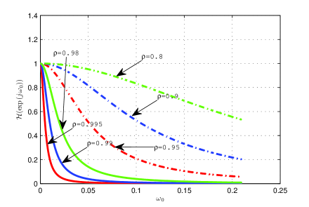
Figure 1: Plot of $\mathcal{H}(\exp(j\omega_{0}))$ in (20) near origin for different values of $\rho$

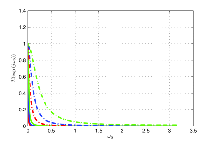
Figure 2: Plot of $\mathcal{H}(\exp(j\omega_{0}))$ in (20) over $[0,\pi]$ for different values of $\rho$. The colour coding is as for Figure 1.

Observe that if $\rho$ is close to 1, i.e. $1-\rho$ is small, a straightforward calculation shows that with $\omega_{0}=1-\rho$, the value of $\mathcal{H}$ is approximately $1/2$. Thus crudely, $\rho$ (for values close to 1) determines the bandwidth as $O(1-\rho)$. More generally, we observe from the Figures 1 and 2 (which show behaviour near the origin and over $[0,\pi]$), that

1. For any $\rho$, $\mathcal{H}(\exp(j\omega_{0}))$ is monotonic decreasing in $\omega_{0}$, from a value of 1 at $\omega_{0}=0$ to a value of $\frac{(1-\rho)^{2}}{(1+\rho)^{2}}$ at $\omega_{0}=\pi$.

2. For values of $1-\rho$ between zero and at least 0.2, $\mathcal{H}(\exp(j\omega_{0}))$ takes a value of about $\frac{1}{2}$ when $\omega_{0}=1-\rho$.

The above calculations assume that there are an infinite number of measuring agents. When the number is finite, it is clear that the results will undergo some variation. When the hop distance to the array boundary, call it $d$, from a particular agent, is such that $\rho^{d}$ is very small, the error will obviously be minor. In the vicinity of the boundary, the errors will be greater, and a kind of end effect will be observed. The results for an infinite number of agents are accordingly indicative of the results for a finite number.

III-B Uniform Finite Window

From (7), the steady-state equation in this case is

$$y_{i}=\frac{1}{2{L}+1}\sum_{k=-{L}}^{L}x_{i+k}$$ (21)

and it is straightforward to establish that

$$\mathcal{Y}(Z)=\frac{1}{2{L}+1}\sum_{k=-{L}}^{L}Z^{k}\mathcal{X}(Z)$$ (22)

The transfer function $\mathcal{H}(Z)$ is simply $\frac{1}{2{L}+1}\sum_{k=-{L}}^{L}Z^{k}$ so that

$$\mathcal{H}(\exp(j\omega))=\frac{1}{2{L}+1}\frac{\sin(({L}+\frac{1}{2})\omega)}{\sin(\omega/2)}$$ (23)

The shape of the Dirichlet kernel is well known; $\mathcal{H}$ assumes its maximum value of 1 at $\omega=0$, and the bandwidth is roughly $\frac{1.7}{L+1/2}$. Evidently, the bandwidths in the exponential weighted case and the uniform finite window case are of the same order when

$$1-\rho=\frac{1.7}{L+1/2}.$$ (24)

Put another way, and roughly speaking, a window length of $2L+1$ allows spatial variation of a bandwidth $\Omega$ to pass through the averaging process when $L\Omega$ is about $1.7$.

IV Noise Propagation

As mentioned already, the noise performance when local consensus is used will be worse than that when global consensus is used. To fix ideas, suppose that for each $i$, measurement agent $i$ has its measurement contaminated by additive noise $\epsilon_{i}$ of zero mean and variance $\sigma^{2}$, with the noise at any two agents being independent.

Then if there are $N$ agents, the error in the average will be $(1/N)\sum_{i=1}^{N}\epsilon_{i}$, which has variance $\frac{\sigma^{2}}{N}$. Obviously this goes to zero as $N\rightarrow\infty$.

When the uniform finite window of length $2{L_{i}}+1$ is used, this same thinking shows that the error variance is $\frac{\sigma^{2}}{2{L_{i}}+1}$.

Now suppose that exponential weighting is used. In local average consensus the error will be

$$\frac{1-\rho}{1+\rho}[\epsilon_{i}+\rho\epsilon_{i-1}+\rho^{2}\epsilon_{i-2}+\dots+\rho\epsilon_{i+1}+\rho^{2}\epsilon_{i+2}+\dots]$$ (25)

and the variance is given by

$$\big{(}\frac{1-\rho}{1+\rho}\big{)}^{2}[1+2\rho^{2}+2\rho^{4}+\dots]\sigma^{2}$$ (26)

$$~{}~{}=\big{(}\frac{1-\rho}{1+\rho}\big{)}^{2}[\frac{2}{1-\rho^{2}}-1]\sigma^{2}$$

$$=(1-\rho)\frac{1+\rho^{2}}{(1+\rho)^{3}}\sigma^{2}$$

This lies in the interval $(\frac{1}{4}(1-\rho),1-\rho))$, and for $\rho$ close to 1, the error is approximately equal to the lower bound. Indeed, the closer $\rho$ is to 1, the less is the error variance. It is not hard to verify that a uniform finite window of length $2{L_{i}}+1$ and an exponential weighting of $\rho=\frac{2{L_{i}}-3}{2{L_{i}}+1}$ yield the same variance. Equivalently, this condition is $1-\rho=\frac{2}{{L_{i}}+1/2}$, which means that exponential weighting and uniform finite window weighting, if they achieve the same bandwidth (cf. (24)), also have approximately the same noise performance. The same condition incidentally says that $\rho^{L_{i}}\approx e^{-1}$, implying that the finite window width with uniform weighting has width determined by the number of steps over which the exponential weighting dies off by a factor of $e$. These observations also mean, unsurprisingly, that when ${L_{i}}$ or $\rho$ are adjusted, noise variance is proportional to bandwidth.

V Generalizations

V-A Arbitrary Weighting

To this point, we have considered two types of weights. It is at least of academic interest to consider what might happen with essentially arbitrary weights. These might for example reflect known and nonuniform spacings between agents. We adopt the following assumption.

Assumption 1.

Let $a_{ij}\neq 0$ for all $i,j$. For every $i$, the following sum

$$a_{ii}x_{i}+\sum_{j=1}^{\infty}(a_{i,i-j}x_{i-j}+a_{i,i+j}x_{i+j})$$ (27)

is finite, and

$$K:=a_{ii}+\sum_{j=1}^{\infty}(a_{i,i-j}+a_{i,i+j}).$$ (28)

Problem 3. Design a distributed algorithm to update each sensor $i$’s consensus variable $y_{i}(k)$ such that

$$\lim_{k\rightarrow\infty}y_{i}(k)=\frac{1}{K}\left(a_{ii}x_{i}+\sum_{j=1}^{\infty}(a_{i,i-j}x_{i-j}+a_{i,i+j}x_{i+j})\right).$$ (29)

The constant $1/K$ ensures again that, if all $x_{i}$ are the same, $y_{i}(k)$ is in the limit equal to $x_{i}$.

To solve Problem 3, we consider a modified approach: Let each sensor $i$ have two additional consensus variables, $y^{F}_{i}(k)$ and $y^{B}_{i}(k)$; $y^{F}_{i}(k)$ (resp. $y^{B}_{i}(k)$) is updated based on $x_{i}$ and information from the forward neighbor $i+1$ (resp. the backward neighbor $i-1$). This approach separates the updates of consensus variables between the forward and the backward directions. As we will see, the separation effectively avoids term cancelations needed in the algorithms in Section II, which we find difficult in the case of arbitrary weights.

Now using the two consensus variables $y^{F}_{i}(k)$ and $y^{B}_{i}(k)$, we present the following distributed algorithm. For all $i$,

$$y^{F}_{i}(0) =y^{B}_{i}(0)=\frac{1}{K}a_{ii}x_{i}$$ (30a)

$$y^{F}_{i}(1) =y^{F}_{i}(0)+\frac{a_{i,i+1}}{a_{i+1,i+1}}y^{F}_{i+1}(0)$$ (30b)

$$y^{B}_{i}(1) =y^{B}_{i}(0)+\frac{a_{i,i-1}}{a_{i-1,i-1}}y^{B}_{i-1}(0)$$

$$y^{F}_{i}(2) =y^{F}_{i}(1)+\frac{a_{i,i+2}}{a_{i+1,i+2}}(y^{F}_{i+1}(1)-y^{F}_{i+1}(0))$$ (30c)

$$y^{B}_{i}(2) =y^{B}_{i}(1)+\frac{a_{i,i-2}}{a_{i-1,i-2}}(y^{B}_{i-1}(1)-y^{B}_{i-1}(0))$$

$$y^{F}_{i}(k+1) =y^{F}_{i}(k)+\frac{a_{i,i+k+1}}{a_{i+1,i+k+1}}(y^{F}_{i+1}(k)-y^{F}_{i+1}(k-1))$$ (30d)

$$y^{B}_{i}(k+1) =y^{B}_{i}(k)+\frac{a_{i,i-k-1}}{a_{i-1,i-k-1}}(y^{B}_{i-1}(k)-y^{B}_{i-1}(k-1)),\ k\geq 2.$$

In the above algorithm, each sensor $i$ requires two consensus variables and needs to know the weights used by its two neighbors, in addition to the memory requirement of the algorithms in Section II. Finally, values of $y^{F}_{i}(k)$ and $y^{B}_{i}(k)$ are glued together to produce $y_{i}(k)$ as follows:

$$y_{i}(k)=y^{F}_{i}(k)+y^{B}_{i}(k)-\frac{1}{K}a_{ii}x_{i},\ \forall k\geq 0.$$ (31)

The last term above serves to correct that the initial $(1/K)a_{ii}x_{i}$ value in (30a) is added twice

Theorem 3.

Let Assumption 1 hold. Then Algorithm (30)-(31) solves Problem 3.

Proof. First, we show by induction on $k\geq 1$ that for all $i$,

$$y^{F}_{i}(k)=y^{F}_{i}(k-1)+\frac{1}{K}a_{i,i+k}x_{i+k}.$$ (32)

It is easily verified from (30b), (30c) that (32) holds when $k=1,2$. Now let $k\geq 2$ and suppose (32) holds for $k$. According to (30d) we derive

$$y^{F}_{i}(k+1)=y^{F}_{i}(k)+\frac{a_{i,i+k+1}}{a_{i+1,i+k+1}}\frac{1}{K}a_{i+1,i+k+1}x_{i+k+1}$$

$$=y^{F}_{i}(k)+\frac{1}{K}a_{i,i+k+1}x_{i+k+1}.$$

Therefore, (32) holds for all $k\geq 1$, and leads to

$$y^{F}_{i}(k) =y^{F}_{i}(0)+\frac{1}{K}\sum_{j=1}^{k}a_{i,i+j}x_{i+j}$$

$$=\frac{1}{K}\left(a_{ii}x_{i}+\sum_{j=1}^{k}a_{i,i+j}x_{i+j}\right),\ \ \forall i.$$

The second equality above is due to (30a). Similarly, for $y^{B}_{i}(k)$, we derive

$$y^{B}_{i}(k)=\frac{1}{K}\left(a_{ii}x_{i}+\sum_{j=1}^{k}a_{i,i-j}x_{i-j}\right),\ \ \forall i.$$

Now by (31),

$$y_{i}(k)=\frac{1}{K}\left(a_{ii}x_{i}+\sum_{j=1}^{k}(a_{i,i-j}x_{i-j}+a_{i,i+j}x_{i+j})\right),\ \ \forall i.$$

Then taking the limit as $k\rightarrow\infty$ yields (29). That the limit exists follows from Assumption 1. $\blacksquare$

V-B Random Spacing

If the arbitrary weights studied in the previous subsection reflect nonuniform distances between successive sensors, we may assume that these distances are random, in accordance with some probability law. Two different possibilities are that (a) they are Poisson distributed, let us say with intensity 1 (assumed for convenience), or (b) the inter sensor distances are uniformly distributed in an interval $[1-\eta,1+\eta]$ where $\eta$ is known. Different physical mechanisms could typically lead to these two situations. In the first case, sensor distances are independent. In the second case, we make the explicit assumption that inter sensor distances are independent random variables.

Based on the treatment already derived for the case corresponding to uniform spacing in Section II-A, where a weighting of $\rho^{d}$ applies at a given sensor to the measurement passed to it and made at a sensor $d$ units away, we suggest that the relevant weighting to apply to the measurement collected at sensor $j$ and used at sensor $i<j$ is, with $d_{i,i+j}$ denoting the distance between sensors $i$ and $i+j$,

$$\rho^{d_{i,i+1}+d_{i+1,i+2}+\dots+d_{j-1,j}}=\rho^{d_{ij}}$$

The full expression for the average consensus variable at node $i$ is then

$$y_{i}=K[x_{i}+\sum_{j=1}^{\infty}\rho^{d_{i,i+j}}x_{i+j}+\sum_{j=1}^{\infty}\rho^{d_{i,i-j}}x_{i-j}]$$ (33)

Here $K$ is a normalization constant. In the sequel, we determine $K$.

In the deterministic case (Section II-A), the normalisation constant ($\frac{1-\rho}{1+\rho}$) was chosen to ensure that if all measured variables had the same value, $a$ say, then the average consensus variable also took the value $a$. In the random case, we can seek this requirement. But it turns out that we can only assure that $E[y_{i}]=a$. It would then be relevant to consider the question of the variance in $y_{i}$. This is also covered below.

Let us now assume $a=1$ for convenience. Then

$$y_{i}=K[1+\sum_{j=1}^{\infty}\rho^{d_{i,i+j}}+\sum_{j=1}^{\infty}\rho^{d_{i,i-j}}]$$ (34)

Define two random variables

$$u=\sum_{j=0}^{\infty}\rho^{d_{i,i+j}},\;\;v=\sum_{j=0}^{\infty}\rho^{d_{i,i-j}}$$ (35)

(Take $d_{i,i}=0$, so that the first summand in each case is $1$.) Then $u,v$ have the same distribution and are independent. It is obvious that

$$y_{i}=K[u+v-1]$$ (36)

This equation makes clear that $y_{i}$ is indeed a random variable, so that $K$ can only be chosen to ensure that $E[y_{i}]=1$. Now observe further that

$$u=1+\rho^{d_{i,i+1}}\sum_{j=1}^{\infty}\rho^{d_{i+1,i+j}}=1+\rho^{d_{i,i+1}}w$$ (37)

where, crucially, $w$ evidently has the same distribution as $u$, but is independent of the random variable $\rho^{d_{i,i+1}}$. Hence there holds

$$E[u]=1+E[\rho^{d_{i,i+1}}]E[u]$$ (38)

whence $E[u]=(1-E[\rho^{d_{i,i+1}}])^{-1}$ and then to assure $E[y_{i}]=1$, equation (36) implies that we need

$$K=\frac{1-E[\rho^{d_{i,i+1}}]}{1+E[\rho^{d_{i,i+1}}]}$$ (39)

Now suppose the distribution of $d_{i,i+1}$ is Poisson with intensity 1, for which the probability density is $e^{-d}$. The expected value of $\rho^{d_{i,i+1}}$ is then easily computed to be $[1-\log\rho]^{-1}$, so that

$$K=\frac{{\color[rgb]{0,0,1}-}\log\rho}{2-\log\rho}$$ (40)

We remark that when $1-\rho$ is small, both $K$ and the expression applicable in the deterministic case, viz. $\frac{1-\rho}{1+\rho}$, are approximately $\frac{1}{2}(1-\rho)$.

If the distribution of $d_{i,i+1}$ is uniform in $[1-\eta,1+\eta]$, then the expected value of $\rho^{d_{i,i+1}}$ is $\frac{1}{2\eta\log\rho}[\rho^{1+\eta}-\rho^{1-\eta}]$, (the limit of which is $\rho$ when $\eta\rightarrow 0$, as expected). The value of $K$ in this case is

$$K=\frac{2\eta\log\rho-(\rho^{1+\eta}-\rho^{1-\eta})}{2\eta\log\rho+\rho^{1+\eta}-\rho^{1-\eta}}.$$ (41)

Once again, one can verify that when $1-\rho$ is small, the expression is approximately $\frac{1}{2}(1-\rho)$.

Now since we can only assure in the event all $x_{i}$ assume the value that $E[y_{i}]$ takes that value, rather than $y_{i}$ itself, it is of interest to consider what the error might be. Guidance as to the error follows from the variance $E(y_{i}-E[y_{i}])^{2}$. We can work out the variance also, in the following way. From (36) and the fact that $u,v$ are independent but with the same distribution, there follows, in obvious notation

$$\sigma_{y}^{2}=2K^{2}\sigma_{u}^{2}$$ (42)

Now if $x,y$ are two independent random variables with $z=xy$, there holds $\sigma_{z}^{2}=\sigma_{x}^{2}\sigma_{y}^{2}+\sigma_{x}^{2}E[y]^{2}+E[x]^{2}\sigma_{y}^{2}$, and using this it follows from (37) and the fact that $\xi:=\rho^{d_{i,i+1}}$ and $w$ are independent, $w$ having the same distribution as $u$, that

$$\sigma_{u}^{2}=\sigma_{\xi}^{2}\sigma_{u}^{2}+\sigma_{\xi}^{2}E[u]^{2}+E[\xi]^{2}\sigma_{u}^{2}$$ (43)

or

$$\sigma_{u}^{2}=\frac{\sigma_{\xi}^{2}E[u]^{2}}{1-\sigma_{\xi}^{2}-E[\xi]^{2}}=\frac{\sigma_{\xi}^{2}E[u]^{2}}{1-E[\xi^{2}]}$$ (44)

It is straightforward to check that

$$E[\xi^{2}] = \frac{1}{1-2\log\rho}$$ (45)

$$\sigma_{\xi}^{2} = \frac{1}{1-2\log\rho}-\frac{1}{(1-\log\rho)^{2}}$$

$$\sigma_{u}^{2} = -\frac{1}{2\log\rho}$$

$$\sigma_{y}^{2} = 2K^{2}\sigma_{u}^{2}=-\frac{\log\rho}{(2-\log\rho)^{2}}$$

which is of the order of $-\log\rho$. When $x:=1-\rho$, this is approximately $x$. Comparing this variance with the error variance arising in $y_{i}$ with deterministic spacing but error variance $\sigma^{2}=1$ of additive noise perturbing each measured variable, we see that the error is of a similar magnitude.

VI Local Consensus with Time-Varying Measurements

We have so far considered time-invariant local measurements. In practice, however, most measured variables are time-varying: e.g. temperature, pollution, and current/voltage in power lines. In this section, we consider that each measurement variable $x_{i}(k)$ is time-varying, i.e. a function of time $k$, and design distributed algorithms to track temporal variations of measurements, in addition to spatial variations.

Note that in typical studies of global average consensus, it is not common to postulate that local variables change over time. Nevertheless, convergence rates are often considered, being identified as exponential, and there are numerous results that seek to identify such rates (see e.g. [26, 5]). The rates themselves are indicative of the bandwidth of variation of measured variables whose average can be tracked by the global consensus algorithms.

In the sequel, we will again consider the two schemes: first exponential weighting, and then uniform finite window.

VI-A Exponential Weighting

Henceforth, we shall assume as is reasonable that there is a bound $M<\infty$ such that measured variables $|x_{i}(k)|<M$ for all $i,k$.

Problem 3. Let $\rho\in(0,1)$. Design a distributed algorithm to update each sensor $i$’s consensus variable $y_{i}(k)$ such that

$$y_{i}(k)=\frac{1-\rho}{1+\rho}\Big{(}x_{i}(k)+\sum_{j=1}^{k}\rho^{j}(x_{i-j}(k-j)+x_{i+j}(k-j))\Big{)}.$$ (46)

Here an exponential weight $\rho^{j}$ is applied to measurements from $j$ steps away sensors in both directions with $j$ time delay. In this way temporal changes of $x_{i}$ are taken into account.

Extending Algorithm (2), we propose the following distributed algorithm, which differs from (2) by inclusion of additional terms reflecting temporal changes in local measurement values.

$$y_{i}(0) =\lambda x_{i}(0),\ \ \lambda:=\frac{1-\rho}{1+\rho}$$ (47a)

$$y_{i}(1) =y_{i}(0)+\rho(y_{i-1}(0)+y_{i+1}(0))+\lambda(x_{i}(1)-x_{i}(0))$$ (47b)

$$y_{i}(2) =y_{i}(1)+\rho(y_{i-1}(1)-y_{i-1}(0))+$$ (47c)

$$\rho(y_{i+1}(1)-y_{i+1}(0))-\rho^{2}2y_{i}(0)+\lambda(x_{i}(2)-x_{i}(1))$$

$$y_{i}(k+1) =y_{i}(k)+\rho(y_{i-1}(k)-y_{i-1}(k-1))+$$ (47d)

$$\rho(y_{i+1}(k)-y_{i+1}(k-1))-\rho^{2}(y_{i}(k-1)-y_{i}(k-2))+$$

$$\lambda(x_{i}(k+1)-x_{i}(k))-\rho^{2}\lambda(x_{i}(k-1)-x_{i}(k-2)),\ k\geq 2.$$

Each sensor $i$ needs information only from its two immediate neighbors: $y_{i-1}(k)$ and $y_{i+1}(k)$, $k=0,1,...$. Note that sensor $i$ does not need its neighbors’ measurement variables $x_{i-1}(k)$ and $x_{i+1}(k)$. Compared to Algorithm (2), two additional quantities (requiring further modest increase in local memory) are used to update $y_{i}(k)$: $x_{i}(k+1)-x_{i}(k)$ and $x_{i}(k-1)-x_{i}(k-2)$; both represent changes in local measurements at different times. As we will see below, $x_{i}(k+1)-x_{i}(k)$ provides new information, while $x_{i}(k-1)-x_{i}(k-2)$ is used as a correction term.

Theorem 4.

Algorithm (47) solves Problem 3.

Proof. It is easily verified from (47b) that $y_{i}(1)=\lambda(x_{i}(1)+\rho(x_{i-1}(0)+x_{i+1}(0)))$ and from (47c) that

$$y_{i}(2) =y_{i}(1)+\rho^{2}(y_{i-2}(0)+y_{i+2}(0))+\lambda\Big{[}(x_{i}(2)-x_{i}(1))$$

$$+\rho\big{(}(x_{i-1}(1)-x_{i-1}(0))+(x_{i+1}(1)-x_{i+1}(0))\big{)}\Big{]}$$ (48a)

$$=\lambda\Big{(}x_{i}(2)+\rho(x_{i-1}(1)+x_{i+1}(1))$$

$$\hskip 19.91684pt+\rho^{2}(x_{i-2}(0)+x_{i+2}(0))\Big{)}$$ (48b)

By (VI-A) we obtain the expressions of $y_{i-1}(2)-y_{i-1}(1)$ and $y_{i+1}(2)-y_{i+1}(1)$; also by (47b) we have $y_{i}(1)-y_{i}(0)$. Substituting these three terms into (47d) yields

$$\begin{split}y_{i}(3)&=y_{i}(2)+\rho^{3}(y_{i-3}(0)+y_{i+1}(0))+\rho^{2}\lambda((x_{i-2}(1)-\\ &x_{i-2}(0))+(x_{i}(1)-x_{i}(0)))+\rho\lambda(x_{i-1}(2)-x_{i-1}(1))+\\ &\rho^{3}(y_{i-1}(0)+y_{i+3}(0))+\rho^{2}\lambda((x_{i}(1)-x_{i}(0))+\\ &(x_{i+2}(1)-x_{i+2}(0)))+\rho\lambda(x_{i+1}(2)-x_{i+1}(1))-\\ &(\rho^{3}((y_{i-1}(0)+y_{i+1}(0)))+\rho^{2}\lambda(x_{i}(1)-x_{i}(0)))+\\ &\lambda(x_{i}(3)-x_{i}(2))-\rho^{2}\lambda(x_{i}(1)-x_{i}(0))\\ &=y_{i}(2)+\rho^{3}(y_{i-3}(0)+y_{i+3}(0))+\lambda\Big{[}(x_{i}(3)-x_{i}(2))\\ &+\rho\big{(}(x_{i-1}(2)-x_{i-1}(1))+(x_{i+1}(2)-x_{i+1}(1))\big{)}+\\ &\rho^{2}\big{(}(x_{i-2}(1)-x_{i-2}(0))+(x_{i+2}(1)-x_{i+2}(0))\big{)}\Big{]}.\end{split}$$ (49)

In deriving the second equality above, the terms $\rho^{3}((y_{i-1}(0)+y_{i+1}(0)))$ and $2\rho^{2}\lambda(x_{i}(1)-x_{i}(0))$ are canceled. Now substituting the expression (48b) of $y_{i}(2)$ into (49), and canceling the terms $\lambda x_{i}(2)$, $\rho\lambda(x_{i-1}(1)+x_{i+1}(1))$, and $\rho^{2}\lambda(x_{i-2}(0)+x_{i+2}(0))$, we derive

$$y_{i}(3)=\lambda\Big{(}x_{i}(3)+\rho(x_{i-1}(2)+x_{i+1}(2))+$$

$$\rho^{2}(x_{i-2}(1)+x_{i+2}(1))+\rho^{3}(x_{i-3}(0)+x_{i+3}(0))\Big{)}.$$

By the same procedure, inductively we can derive $y_{i}(k)$ for $k=4,5,...$, and conclude that (46) holds for all $k$. $\blacksquare$

As commented in Remark 1 for Algorithm (2), we may similarly extend Algorithm (47) to the case where sensors assign different exponential weights to information from the backward and the forward directions, using $\rho_{b},\rho_{f}\in(0,1)$.

VI-B Uniform Finite Window

The finite window case with time-varying measurements is challenging, because all information outside the window has to be discarded, and temporal variations of information within the window have to be tracked. We state the problem formally.

Problem 4. Let $L\geq 1$ be an integer, and $2L+1$ the length of the finite window of sensor $i$; i.e. sensor $i$ uses measurement information from $L$ neighbors in each direction. Suppose $i$ knows $L$. Design a distributed algorithm to update each $i$’s consensus variable $y_{i}(k)$ such that

$$\begin{split}y_{i}(k)&=\frac{1}{2L+1}\left(x_{i}(k)+\sum_{j=1}^{k}(x_{i-j}(k-j)+x_{i+j}(k-j))\right)\\ &\hskip 142.26378pt\mbox{if $k\leq L$;}\\ y_{i}(k)&=\frac{1}{2L+1}\left(x_{i}(k)+\sum_{j=1}^{L}(x_{i-j}(k-j)+x_{i+j}(k-j))\right)\\ &\hskip 142.26378pt\mbox{if $k>L$.}\end{split}$$ (50)

The explanation for the time arguments associated with $x_{i-j}$ and $x_{i+j}$ on the right of (50) is as follows. At each time step, values can be ‘passed’ by exactly one hop. Hence, it takes $j$ time instances for a measured variable at sensor $i-j$ to be perceived at sensor $j$. Therefore the consensus variable $y_{i}(k)$ can depend on $x_{i-j}(k-j)$ (resp. $x_{i+j}(k-j)$ but no later value of $x_{i-j}(k-j)$ (resp. $x_{i+j}(k-j)$).

The distributed algorithm we design to solve Problem 4 has several features. First, it needs an additional vector of variables $z_{i}=[z_{i0}\ z_{i1}\ \cdots\ z_{i(L)}]^{T}$ of $L+1$ components for each sensor $i$, and $z_{i}$ needs to be updated along with consensus variable $y_{i}$ and communicated to the two immediate neighbors $i-1$ and $i+1$. Second, the scheme for each component of $z_{i}$ is similar to Algorithm (8). Finally, we will see that the $j$th component $z_{ij}$, $j\in[0,L]$, contributes to tracking all local measurements $x_{l}(k)$, $l\in[i-L,i+L]$, in the finite window for time $k=j\ (\mbox{mod }L+1)$.

We first present the update scheme for vector $z_{i}$ (c.f. Algorithm (8)). For every $j\in[0,L]$, if $k<j$,

$$z_{ij}(k)=0;$$ (51)

if $k\geq j$ and $k=j\ (\mbox{mod }L+1)$,

$$z_{ij}(k) =\frac{1}{2L+1}x_{i}(k),$$ (52a)

$$z_{ij}(k+1) =z_{ij}(k)+(z_{(i-1)j}(k)+z_{(i+1)j}(k))$$ (52b)

$$z_{ij}(k+2) =z_{ij}(k+1)+(z_{(i-1)j}(k+1)-z_{(i-1)j}(k))$$ (52c)

$$\hskip 8.5359pt+(z_{(i+1)j}(k+1)-z_{(i+1)j}(k))-2z_{ij}(k)$$

$$z_{ij}(k+3) =z_{ij}(k+2)+(z_{(i-1)j}(k+2)-z_{(i-1)j}(k+1))$$ (52d)

$$+(z_{(i+1)j}(k+2)-z_{(i+1)j}(k+1))-(z_{ij}(k+1)-z_{ij}(k))$$

$$\ \ \vdots$$ (52e)

$$z_{ij}(k+L) =z_{ij}(k+L-1)+$$ (52f)

$$(z_{(i-1)j}(k+L-1)-z_{(i-1)j}(k+L-2))+$$

$$(z_{(i+1)j}(k+L-1)-z_{(i+1)j}(k+L-2))-$$

$$(z_{ij}(k+L-2)-z_{ij}(k+L-3))$$

The update of each component $z_{ij}$, $j\in[0,L]$, is periodic with period $L+1$ for $k\geq j$. The following is the update scheme for consensus variable $y_{i}$.

$$\begin{split}y_{i}(k)&=z_{ij}(k)+\sum_{l=0,l\neq j}^{L}(z_{il}(k)-z_{il}(k-1)),\\ &\hskip 99.58464ptj=k\ (\mbox{mod }L+1).\end{split}$$ (53)

Example. We provide an example to explain the above algorithm. Let $L=2$. Then the vector $z_{i}=[z_{i0}\ z_{i1}\ z_{i2}]^{T}$, for all $i$. At $k=0$, the first variable $z_{i0}$ is used to record the current measurement $x_{i}(0)$:

$$z_{i0}(0) =\frac{1}{2L+1}x_{i}(0)\ \ \ \mbox{by (\ref{alg_var_winza})}$$

$$z_{i1}(0) =z_{i2}(0)=0\ \ \ \mbox{by (\ref{alg_var_win_init})}$$

$$y_{i}(0) =z_{i0}(0)=\frac{1}{2L+1}x_{i}(0)\ \ \ \mbox{by (\ref{alg_var_win_y})}$$

At $k=1$, $z_{i0}$ fetches measurements at $k=0$ from 1-hop neighbors, and meanwhile the second variable $z_{i1}$ is used to record the current measurement $x_{i}(1)$:

$$z_{i0}(1) =z_{i0}(0)+(z_{(i-1)0}(0)+z_{(i+1)0}(0))\ \ \ \mbox{by (\ref{alg_var_winzb})}$$

$$=z_{i0}(0)+\frac{1}{2L+1}(x_{i-1}(0)+x_{i+1}(0))$$

$$z_{i1}(1) =\frac{1}{2L+1}x_{i}(1)\ \ \ \mbox{by (\ref{alg_var_winza})}$$

$$z_{i2}(0) =0\ \ \ \mbox{by (\ref{alg_var_win_init})}$$

$$y_{i}(1) =z_{i1}(1)+(z_{i0}(1)-z_{i0}(0))\ \ \ \mbox{by (\ref{alg_var_win_y})}$$

$$=\frac{1}{2L+1}\left(x_{i}(1)+(x_{i-1}(0)+x_{i+1}(0))\right)$$

At $k=2$, $z_{i0}$ fetches measurements at $k=0$ from 2-hop neighbors, $z_{i1}$ fetches measurements at $k=1$ from 1-hop neighbors, and meanwhile the third variable $z_{i2}$ is used to record the current measurement $x_{i}(2)$:

$$z_{i0}(2) =z_{i0}(1)+(z_{(i-1)0}(1)-z_{(i-1)0}(0))+$$

$$\hskip 11.38092pt(z_{(i+1)0}(1)-z_{(i+1)0}(0))-2z_{i0}(0)\ \ \ \mbox{by (\ref{alg_var_winzc})}$$

$$=z_{i0}(1)+(z_{(i-2)0}(0)+z_{(i+2)0}(0))$$

$$=z_{i0}(1)+\frac{1}{2L+1}(x_{i-2}(0)+x_{i+2}(0))$$

$$z_{i1}(2) =z_{i1}(1)+(z_{(i-1)1}(1)+z_{(i+1)1}(1))\ \ \ \mbox{by (\ref{alg_var_winzb})}$$

$$=z_{i1}(1)+\frac{1}{2L+1}(x_{i-1}(1)+x_{i+1}(1))$$

$$z_{i2}(2) =\frac{1}{2L+1}x_{i}(2)\ \ \ \mbox{by (\ref{alg_var_winza})}$$

$$y_{i}(2) =z_{i2}(2)+(z_{i1}(2)-z_{i1}(1))+(z_{i0}(2)-z_{i0}(1))\ \ \ \mbox{by (\ref{alg_var_win_y})}$$

$$=\frac{1}{2L+1}(x_{i}(2)+(x_{i-1}(1)+x_{i+1}(1))+$$

$$\hskip 42.67912pt(x_{i-2}(0)+x_{i+2}(0)))$$

Since $L=2$, information is discarded beyond 2-hop neighbors that are outside of the finite window. Therefore the first variable $z_{i0}$ has completed its first update cycle for measurements made at $k=0$. Now at $k=3$, a new measurement $x_{i}(3)$ is made, and $z_{i0}$ is set to record this current value. The second variable $z_{i1}$ continues to fetch measurements at $k=1$ from 2-hop neighbors, and $z_{i2}$ fetches measurements at $k=2$ from 1-hop neighbors:

$$z_{i0}(3) =\frac{1}{2L+1}x_{i}(3)\ \ \ \mbox{by (\ref{alg_var_winza})}$$

$$z_{i1}(3) =z_{i1}(2)+(z_{(i-1)1}(2)-z_{(i-1)1}(1))+$$

$$\hskip 11.38092pt(z_{(i+1)1}(2)-z_{(i+1)1}(1))-2z_{i1}(1)\ \ \ \mbox{by (\ref{alg_var_winzc})}$$

$$=z_{i1}(2)+(z_{(i-2)1}(1)+z_{(i+2)1}(1))$$

$$=z_{i1}(2)+\frac{1}{2L+1}(x_{i-2}(1)+x_{i+2}(1))$$

$$z_{i2}(3) =z_{i2}(2)+(z_{(i-1)2}(2)+z_{(i+1)2}(2))\ \ \ \mbox{by (\ref{alg_var_winzb})}$$

$$=z_{i2}(2)+\frac{1}{2L+1}(x_{i-1}(2)+x_{i+1}(2))$$

$$y_{i}(3) =z_{i0}(3)+(z_{i2}(3)-z_{i2}(2))+(z_{i1}(3)-z_{i1}(2))\ \ \ \mbox{by (\ref{alg_var_win_y})}$$

$$=\frac{1}{2L+1}(x_{i}(3)+(x_{i-1}(2)+x_{i+1}(2))+$$

$$\hskip 42.67912pt(x_{i-2}(1)+x_{i+2}(1)))$$

The updates continue in the fashion that each of the three variables $z_{i0},z_{i1},z_{i2}$ executes Algorithm (8) once in each period of $3\ (=L+1)$ time instants:

$$z_{i0}:\ \ k\in[0,2],\ [3,5],\ [6,8],\ \cdots$$

$$z_{i1}:\ \ k\in[1,3],\ [4,6],\ [7,9],\ \cdots$$

$$z_{i2}:\ \ k\in[2,4],\ [5,7],\ [8,10],\ \cdots$$

These update cycles are so aligned that each measurement made at a time is taken care by exactly one variable. Note that the updates of each variable is independent, in the sense that the value of one variable does not affect the update of another variable.

We now state the main result of this subsection.

Theorem 5.

Algorithm (51)-(53) solves Problem 4.

Proof. First, at $k=0$, we have from (51), (52a) that $z_{i0}(0)=(1/(2L+1))x_{i}(0)$ and $z_{ij}(0)=0$, $j=1,...,L$. So by (53) $y_{i}(0)=z_{i0}(0)=(1/(2L+1))x_{i}(0)$.

Let $k\geq 1$ and fix $j=k\ (\mbox{mod }L+1)$. Similar to the proof of Theorem 2, in particular Equation (9), we derive

$$z_{ij}(k) =\frac{1}{2L+1}x_{i}(k)\ \ \ \ \ (\mbox{again by (\ref{alg_var_winza})})$$

$$z_{i(j-1)}(k) =z_{i(j-1)}(k-1)+(z_{(i-1)(j-1)}(k-1)+$$

$$\hskip 79.6678ptz_{(i+1)(j-1)}(k-1))$$

$$=z_{i(j-1)}(k-1)+\frac{1}{2L+1}(x_{i-1}(k-1)+x_{i+1}(k-1))$$

$$z_{i(j-2)}(k) =z_{i(j-2)}(k-1)+(z_{(i-2)(j-2)}(k-2)+$$

$$\hskip 79.6678ptz_{(i+2)(j-2)}(k-2))$$

$$=z_{i(j-2)}(k-1)+\frac{1}{2L+1}(x_{i-2}(k-2)+x_{i+2}(k-2))$$

$$\ \ \vdots$$

$$z_{i0}(k) =z_{i0}(k-1)+(z_{(i-j)0}(k-j)+z_{(i+j)0}(k-j))$$

$$=z_{i0}(k-1)+\frac{1}{2L+1}(x_{i-j}(k-j)+x_{i+j}(k-j)).$$

Now if $k\leq L$ (thus $j=k$), then by (51) $z_{i(j+1)}(k)=\cdots=z_{i(L)}(k)=0$. Therefore by (53),

$$y_{i}(k) =z_{ij}(k)+\sum_{l=0}^{j-1}(z_{il}(k)-z_{il}(k-1))$$

$$=\frac{1}{2L+1}\left(x_{i}(k)+\sum_{j=1}^{k}(x_{i-j}(k-j)+x_{i+j}(k-j))\right).$$

This is the first part of (50).

If $k>L$, then again similar to Equation (9) we derive

$$z_{i(L)}(k) =z_{i(L)}(k-1)+(z_{(i-j-1)(L)}(k-j-1)+$$

$$\hskip 76.82234ptz_{(i+j+1)(L)}(k-j-1))$$

$$=z_{i(L)}(k-1)+\frac{1}{2L+1}(x_{i-j-1}(k-j-1)+$$

$$\hskip 108.12054ptx_{i+j+1}(k-j-1))$$

$$\ \ \vdots$$

$$z_{i(j+1)}(k) =z_{i(j+1)}(k-1)+(z_{(i-L)(j+1)}(k-L)+$$

$$\hskip 82.51282ptz_{(i+L)(j+1)}(k-L))$$

$$=z_{i(j+1)}(k-1)+\frac{1}{2L+1}(x_{i-L}(k-L)+$$

$$\hskip 113.81102ptx_{i+L}(k-L)).$$

Therefore by (53),

$$y_{i}(k) =z_{ij}(k)+\sum_{l=0,l\neq j}^{L}(z_{il}(k)-z_{il}(k-1))$$

$$=\frac{1}{2L+1}\left(x_{i}(k)+\sum_{j=1}^{L}(x_{i-j}(k-j)+x_{i+j}(k-j))\right).$$

This is the second part of (50), and thus completes the proof.

$\blacksquare$

In the next section, we analyze the frequency response for the two local consensus algorithms designed in this section, with respect to both spatial and temporal variations.

VII Temporal Frequency Response

In this section, we consider the question of how changes in the measured variables propagate to become changes in the consensus variables. Specifically, we consider how sinusoidal variations in measured variables reflects through, as a function of frequency, to time-variation of the local consensus variables. As with the case of spatial variation, we are interested in understanding what speed of variations might be trackable by the local average consensus algorithm, through the identification of a transfer function and its associated bandwidth. This question is rather understudied for global consensus.

We shall first consider a special situation, viz. one where there is no spatial variation, but merely sinusoidal time-variation, i.e. for all $i$, there holds $x_{i}(k)=e^{j\omega_{0}k}$. Recall that in studying spatial variation, we considered the special case where there was no time-variation. Studying these special situations allow clearer examination of the separate effects of time-variation and spatial variation.

Now when values are independent of the spatial index $i$, equation (47d) yields

$$y_{i}(k+1) =(1+2\rho)y_{i}(k)-(2\rho+\rho^{2})y_{i}(k-1)+\rho^{2}y_{i}(k-2)$$

$$+\frac{1-\rho}{1+\rho}[x_{i}(k+1)-x_{i}(k)+-\rho^{2}(x_{i}(k-1)-x_{i}(k-2))]$$ (54)

The transfer function linking the measured to consensus variables is then

$$\mathcal{K}(e^{j\omega}) =\frac{\frac{1-\rho}{1+\rho}[1-e^{-j\omega}-\rho^{2}(e^{2j\omega}-e^{3j\omega})]}{1-(1+2\rho)e^{-j\omega}+(2\rho+\rho^{2})e^{-2j\omega}-\rho^{2}e^{-3j\omega}}$$

$$=\frac{\frac{1-\rho}{1+\rho}[1-\rho^{2}e^{-2j\omega}]}{1-2\rho e^{-j\omega}+\rho^{2}e^{-2j\omega}}$$

$$=\frac{\frac{1-\rho}{1+\rho}[1-\rho^{2}e^{-2j\omega}]}{(1-\rho e^{-j\omega})^{2}}$$ (55)

Evidently, the transfer functions $\mathcal{K}(e^{j\omega})$ and $\mathcal{H}(e^{j\omega})$ in (20) are not that different in terms of the way their magnitude depends on $\omega$ and $\rho$. Indeed, once again one can verify that if $1-\rho$ is small and $\omega=1-\rho$, then $\mathcal{K}$ is approximately $1/2$. So the spatial and temporal bandwidths are about the same. This appears consistent with the assumption that a spatial progression of one hop occurs in each time update, i.e. values propagate with effectively unit velocity. Of course, the poles and zeros for the spatial transfer function lie symmetrically inside and outside the unit circle, in contrast to the time-based frequency response. We display the behaviour of $\mathcal{K}(e^{j\omega})$ near the origin and over $[0,\pi]$ respectively in Figures 3 and 4.

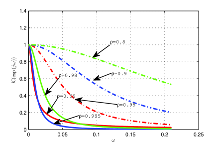
Figure 3: Plot of $\mathcal{K}(\exp(j\omega))$ in (VII) near origin for different values of $\rho$

Figure 4: Plot of $\mathcal{K}(\exp(j\omega))$ in (VII) over $[0,\pi]$ for different values of $\rho$. The colour coding is as for Figure 3.

The treatment of time variation when the uniform finite window approach is being used is also simple. Analogously to (VII), we can obtain for

$$\mathcal{K}^{\prime}(e^{j\omega})=\frac{1}{2L+1}[1+2(e^{-j\omega}+e^{-2j\omega}+\cdots+e^{-Lj\omega})]$$ (56)

Figure 5 shows plots of this expression for different values of $L$. When $\frac{2}{L+1/2}$ is small (this corresponds to the condition $1-\rho$ is small for the exponential weighting case), we can see that the frequency at which $|\mathcal{K}^{\prime}(e^{j\omega})|$ assumes the value $1/2$ is approximately $\frac{4}{L+1/2}$.

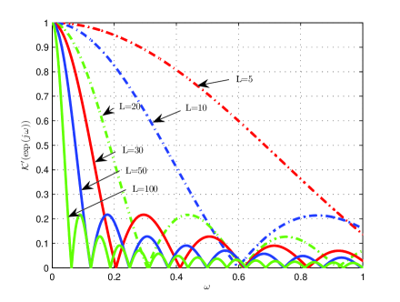
Figure 5: Plot of $\mathcal{K}^{\prime}(\exp(j\omega))$ in (56) for different values of $L$.

Finally, we remark that the considerations applicable to spatial variation without temporal variation or to temporal variation without spatial variation will apply (because of the linearity of the whole system) to a situation where both types of variation are present in the measured variables. Thus if the measured variable variation places them in the spatial bandwidth and outside the temporal bandwidth, or the reverse, the consensus averaging process will attenuate or suppress the variation.

VIII Conclusions

We have studied local average consensus in distributed measurement of a variable using 1D sensor networks. Distributed local consensus algorithms have been designed to address first the case where the measured variable has spatial variation but is constant in time, and then the case where the measured variable has both spatial and temporal variations. Two schemes for local average computation have been employed: exponential weighting and uniform finite window. Further, we have analyzed temporal-spatial frequency response and noise propagation associated to the algorithms. Arbitrary updating weights and random spacing between sensors have been analyzed in the proposed algorithms.

In work which has yet to be submitted for publication, we have studied two dimensional arrays. With a uniform grid, results rather like those with fixed $\rho$ and $L$ can be obtained, but for a general two dimensional array, a theory appears needed and is currently under development.

IX ACKNOWLEDGMENTS

This research is supported by ARC Discovery projects DP110100538 and DP120102030. National ICT Australia (NICTA) is funded by the Australian Government as represented by the Department of Broadband, Communications and the Digital Economy and the Australian Research Council through the ICT Centre of Excellence program.

References

- [1] D. P. Bertsekas and J. N. Tsitsiklis, Parallel and Distributed Computation: Numerical Methods. Prentice Hall, 1989.
- [2] A. Jadbabaie, J. Lin, and A. S. Morse, “Coordination of groups of mobile autonomous agents sing nearest neighbor rules,” IEEE Trans. Autom. Control, vol. 48, no. 6, pp. 988–1001, 2003.
- [3] L. Moreau, “Stability of multi-agent systems with time dependent communication links,” IEEE Trans. Autom. Control, vol. 50, no. 2, pp. 169–182, 2005.
- [4] W. Ren, R. W. Beard, and E. M. Atkins, “Information consensus in multivehicle cooperative control,” IEEE Control Systems Magazine, vol. 27, no. 2, pp. 71–82, 2007.
- [5] R. Olfati-Saber, J. A. Fax, and R. M. Murray, “Consensus and cooperation in networked multi-agent systems,” Proc. IEEE, vol. 95, no. 1, pp. 215–233, 2007.
- [6] R. Olfati-Saber and R. M. Murray, “Consensus problems in networks of agents with switching topology and time-delays,” IEEE Trans. Autom. Control, vol. 49, no. 9, pp. 1520–1533, 2004.
- [7] S. Boyd, A. Ghosh, B. Prabhakar, and D. Shah, “Randomized gossip algorithms,” IEEE Trans. Inform. Theory, vol. 52, no. 6, pp. 2508–2530, 2006.
- [8] L. Xiao, S. Boyd, and S.-J. Kim, “Distributed average consensus with least-mean-square deviation,” J. of Parallel and Distributed Computing, vol. 67, no. 1, pp. 33–46, 2007.
- [9] K. Cai and H. Ishii, “Average consensus on general strongly connected digraphs,” Automatica, vol. 48, no. 11, pp. 2750–2761, 2012.
- [10] K. Topley and V. Krishnamurthy, “Average-consensus in a deterministic framework–part I: strong connectivity,” IEEE Trans. Sig. Processing, vol. 60, no. 12, pp. 6590–6603, 2012.
- [11] S. Kar and J. Moura, “Distributed consensus algorithms in sensor networks with imperfect communication: link failures and channel noise,” IEEE Trans. Sig. Processing, vol. 57, no. 1, pp. 355–369, 2009.
- [12] S. Lovisari and S. Zampieri, “Performance metrics in the consensus problem: a survey,” in Proc. 4th IFAC Symp. on System, Structure and Control, 2010, pp. 324–335.
- [13] X. Liu, W. Lu, and T. Chen, “Consensus of multi-agent systems with unbounded time-varying delays,” IEEE Trans. Autom. Control, vol. 55, no. 10, pp. 2396–2401, 2010.
- [14] Y. Zhang and Y. Tian, “Maximum allowable loss probability for consensus of multi-agent systems over random weighted lossy networks,” IEEE Trans. Autom. Control, vol. 57, no. 8, pp. 2127–2132, 2012.
- [15] H. Gharavi and S. K. G. Editors), “Special issue on sensor networks and applications,” Proc. IEEE, vol. 91, no. 8, 2003.
- [16] Y. Chen and J. Hwang, “A power-line-based sensor network for proactive electrical fire precaution and early discovery,” IEEE Trans. Power Delivery, vol. 23, no. 2, pp. 633–639, 2008.
- [17] B. Huang, C. Yu, and B. Anderson, “Analyzing localization errors in one-dimensional sensor networks,” Sig. Processing, vol. 92, no. 2, p. 427 438, 2012.
- [18] M. Arik and O. B. Akan, “Collaborative mobile target imaging in UWB wireless radar sensor networks,” IEEE J. Selected Areas in Communications, vol. 28, no. 6, pp. 950–961, 2010.
- [19] S. Yoon, W. Ye, J. Heidemann, B. Littlefield, and C. Shahabi, “Swats: wireless sensor networks for steamflood and waterflood pipeline monitoring,” IEEE Trans. Sig. Processing, vol. 55, no. 2, pp. 684–696, 2007.
- [20] R. Olfati-Saber and J. S. Shamma, “Consensus filters for sensor networks and distributed sensor fusion,” in Proc. 44th IEEE Conf. on Decision and Control and Eur. Control Conf., Seville, Spain, 2005, pp. 6698–6703.
- [21] R. A. Freeman, P. Yang, and K. M. Lynch, “Stability and convergence properties of dynamic average consensus estimators,” in Proc. 45th IEEE Conf. Decision and Control, San Diego, CA, 2006, pp. 338–343.
- [22] H. Bai, R. A. Freeman, and K. M. Lynch, “Robust dynamic average consensus of time-varying inputs,” in Proc. 49th IEEE Conf. Decision and Control, Atlanta, GA, 2010, pp. 3104–3109.
- [23] Y. Hong, J. Hu, and L. Gao, “Tracking control for multi-agent consensus with an active leader and variable topology,” Automatica, vol. 42, no. 7, pp. 1177–1182, 2006.
- [24] Y. Cao, W. Ren, and Y. Li, “Distributed discrete-time coordinated tracking with a time-varying reference state and limited communication,” Automatica, vol. 45, no. 5, pp. 1299–1305, 2009.
- [25] H. Bai, M. Arcak, and J. T. Wen, “Adaptive motion coordination: using relative velocity feedback to track a reference velocity,” Automatica, vol. 45, no. 4, pp. 1020–1025, 2009.
- [26] L. Xiao and S. Boyd, “Fast linear iterations for distributed averaging,” Systems & Control Letters, vol. 53, no. 1, pp. 65–78, 2004.