A volume-of-fluid formulation for the study of co-flowing fluids governed by the Hele-Shaw equations

Abstract

We present a computational framework to address the flow of two immiscible viscous liquids which co-flow into a shallow rectangular container at one side, and flow out into a holding container at the opposite side. Assumptions based on the shallow depth of the domain are used to reduce the governing equations to one of Hele-Shaw type. The distinctive feature of the numerical method is the accurate modeling of the capillary effects. A continuum approach coupled with a volume-of-fluid formulation for computing the interface motion and for modeling the interfacial tension in Hele-Shaw flows are formulated and implemented. The interface is reconstructed with a height-function algorithm. The combination of these algorithms is a novel development for the investigation of Hele-Shaw flows. The order of accuracy and convergence properties of the method are discussed with benchmark simulations. A microfluidic flow of a ribbon of fluid which co-flows with a second liquid is simulated. We show that for small capillary numbers of O(0.01), there is an abrupt change in interface curvature and focusing occurs close to the exit.

I Introduction

Microfluidic devices for droplet production are often based on forcing a jet of one liquid sandwiched in another liquid through a series of channels Anna, Bontoux, and Stone (2003); De Menech (2006); Rotem et al. (2012); Seemann et al. (2012). The investigation of the transition between a stable jet and its breakup into a stream of droplets is a model paradigm for the much needed control of co-flowing systems, ubiquitous in current technological applications. Regimes for stable jets and unstable dripping jets are being studied experimentally, with theoretical models, and numerical simulations Guillot et al. (2007); Utada et al. (2007); Couture et al. (2011); Lei and Wang (2011). The breakup of a liquid jet into ever smaller and more complex droplets includes the experimental investigation of the effects of relative sizes of the channels, as well as channel geometry. An attractive experimental technique is recently addressed for a channel which is shallow compared to its width and length, emptying into a larger channel. The shallow area forces the jet to become a ribbon rather than a cylinder, and the ribbon remains stable until it flows into a holding tank. In this light, the suppression of instabilities in multiphase flow by geometric confinement is studied in Ref. Humphry et al., 2009, where the experimental work on decreasing the depth of the channel and simplified estimates are compared to conclude that when the depth is sufficiently shallow, the ribbon is stabilized. This idea is used for a single step emulsification Priest, Herminghaus, and Seemann (2006); Malloggi et al. (2010).

In Ref. Malloggi et al., 2010, experimental data for step emulsification are compared with a model for the size of the drops that emerge at the step where the ribbon flows into a deeper tank, where the cylindrical necking takes place. Although this is proving to be one of the simplest methods to rapidly produce droplets with controllable sizes and morphologies Shui, van den Berg, and Eijkel (2011); Adams et al. (2012), the optimal operating conditions are not entirely understood.

The numerical simulation of a ribbon or jet sheathed in another liquid, pressure-driven and co-flowing through a shallow channel, is a time-dependent simulation because of the kinematic free surface condition, and the solution quickly reaches a steady state. A first step toward understanding the main features is to take advantage of the smallness of the depth of the channel compared with the other dimensions. Thus, the original governing equations are reduced to the Hele-Shaw equations. The key assumptions are given in Sec. II. Our volume-of-fluid (VoF) formulation uses the balanced-force height-function (HF) formulation of Ref. Afkhami and Bussmann, 2008. The accuracy for modeling the capillary effects is highlighted in this reference. Our implementation is developed for a more general class of Hele-Shaw flows of two immiscible viscous liquids than that considered in this paper, and is novel for the particular regime where the interfacial tension force is dominant. The quad-tree adaptive mesh refinementPopinet (2003); Afkhami and Bussmann (2008, 2009) is enforced in regions where much of the important dynamics takes place. The balanced-force HF method has the feature of reaching an equilibrium solution without spurious solutions Renardy and Renardy (2002); Francois et al. (2006); Afkhami and Bussmann (2009). For an overview of methods for surface-tension dominated multiphase flows, and recent developments, including the phase-field method and the level-set method, the reader is referred to recent publications Hou, Lowengrub, and Shelley (2001); Tryggvason, Scardovelli, and Zaleski (2011); Khatri and Tornberg (2011).

In Sec. III, we present our numerical methodology. Benchmark computations are given in Sec. IV. These results form a baseline and a standard for numerical accuracy. This is followed in Sec. V with numerical simulations for the experimental conditions of Ref. Malloggi et al., 2010. This reference derives a formula for the size of the neck at the outlet, as a first step toward understanding the mechanism of capillary focusing. However, this is not a closed formula, and requires empirical input, because certain assumptions were made to arrive at a tractable model. Basically, the model reflects inflow and outflow flux balances. We perform numerical simulations in order to investigate whether the flowfield satisfies those assumptions.

II Governing equations for a volume-of-fluid formulation

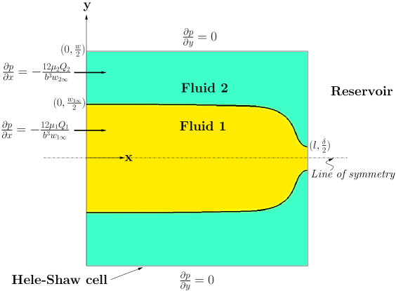
Figure 1: Schematic of the flow domain for the Hele-Shaw model. The depth is small compared to the width $w$ in the $y$-direction and the length of the domain $\ell$ in the $x$-direction. At $x=0$, Fluid 1 occupies $|y|\leq\frac{w_{1\infty}}{2}$ and Fluid 2 occupies $\frac{w_{1\infty}}{2}\leq|y|\leq\frac{w}{2}$; $w_{2\infty}=w-w_{1\infty}$. The flow is driven by $\frac{\partial p}{\partial x}$, which is related to the flow rates $Q_{i}$ for Fluid $i$, $i=1,2$. The fluids exit at $x=\ell$, where the width $\delta$ of Fluid 1 must be determined as part of the solution. The domain is bounded by walls at $|y|=\frac{w}{2}$.

Figure 1 is a schematic of the flow domain, $0\leq x\leq\ell$, $|y|\leq\frac{w}{2}$. The depth $b$ in the z-direction is small compared with the width $w$ and the length $\ell$. The jet and surrounding liquid are separated by a wall for $x<0$, and pumped under pressure through the boundary at $x=0$. At the exit $x=\ell$, the width of the jet is unknown and is denoted by $\delta$. The exit boundary condition is constant pressure $P_{0}$, which is a first approximation for the outflow into a reservoir. Capillary effects are expected to decrease the jet width across the domain. The governing equations prior to a Hele-Shaw approximation are the 3D Stokes equations and incompressibility

$${\bf 0}=-\nabla p(x,y,z,t)+\mu\nabla^{2}{\bf v}(x,y,z,t)+{\bf F}_{ST},\quad\nabla\cdot{\bf v}(x,y,z,t)=0,$$ (1)

where ${\bf v}=(v_{1},v_{2},v_{3})$, ${\bf F}_{ST}$ denotes the body force with the continuum surface tension formulation Brackbill, Kothe, and Zemach (1992), and the viscosity of Fluid $i$ is $\mu=\mu_{i}$, $i=1,2$. Fluid 1 occupies $\Omega_{1}=\{(x,y,z):0\leq x\leq\ell,|y|\leq h(x,t)<\frac{w}{2},0\leq z\leq b\}$. Fluid 2 occupies $\Omega_{2}=\{(x,y,z):0\leq x\leq\ell,h(x,t)\leq|y|<\frac{w}{2},0\leq z\leq b\}$. We denote $\Omega_{1}\cup\Omega_{2}=\Omega\subset\mathbb{R}^{3}$.

The volume-of-fluid formulation identifies each fluid by assigning a VoF function,

$$\tilde{f}(x,y,z,t) = \left\{\begin{array}[]{ll}1&\mbox{in Fluid 1}\\ 0&\mbox{in Fluid 2}.\end{array}\right.$$ (4)

The interface is calculated by reconstructing the curve where the step discontinuity takes place.

The sign convention of ${\bf F}_{ST}$ stems from our equilibrium state for (1) where Fluid 1 (the jet) bulges into Fluid 2. Since the pressure in Fluid 1 is higher than in Fluid 2, $\nabla p$ points into Fluid 1. The unit normal ${\bf n}=\nabla\tilde{f}/|\nabla\tilde{f}|$ also points into Fluid 1. Therefore,

$${\bf F}_{ST}=\gamma\kappa\delta_{S}{\bf n},$$ (5)

where $\delta_{S}(x,y,z)$ $=|\nabla\tilde{f}(x,y,z,t)|$ at the interface $S$ in the distribution sense Renardy and Rogers (2004). The curvature is

$$\kappa=-\nabla\cdot{\bf n},$$ (6)

where $\nabla\cdot{\bf n}<0$ if the interface bulges into the direction $-{\bf n}$ (into Fluid 2), and $>0$ otherwise. The fluids are advected by the velocity field;

$$\frac{\partial\tilde{f}(x,y,z,t)}{\partial t}+({\bf v}\cdot\nabla)\tilde{f}(x,y,z,t)=0.$$ (7)

II.1 The 2D Hele-Shaw approximation

Although the 2D Hele-Shaw equations are well known Ockendon and Ockendon (1995), we remind the reader of the key ideas in the context of a two-fluid flow.

1. In the momentum equation for the $x$-$y$ plane, $\rho\frac{D{\bf v}}{Dt}$ is assumed to be negligible compared with $\nabla p$ and $\nabla^{2}{\bf v}$. The assumption is that $b$ is small, so that $\nabla^{2}\sim\frac{\partial^{2}}{\partial z^{2}}=O(\frac{1}{b^{2}})$. This means $p=O(\frac{1}{b^{2}})$. Thus, $\rho\frac{D{\bf v}}{Dt}$ in the $x$-$y$ plane is assumed to be smaller order than $O(\frac{1}{b^{2}})$.

2. The vertical depth between the walls, $b$, is assumed small compared with the length of the walls in the $x$-direction, $\ell$, and the width $w$ in the $y$-direction: $\frac{b}{w}\ll 1,\frac{b}{\ell}\ll 1$. The components of the velocity have magnitudes $v_{1}=O(1)$, $v_{2}=O(1)$, $v_{3}=O(b)$. We define an in-plane depth-averaged velocity field ${\bf V}=(V_{1}(x,y,t),V_{2}(x,y,t))$,

   $${\mathbf{V}}(x,y,t)=\frac{1}{b}\int_{0}^{b}(v_{1}(x,y,z,t),v_{2}(x,y,z,t))dz.$$ (8)

3. The out-of-plane interface shape is assumed to be semi-circular, with contact angle 180^o at the walls, and radius $b/2$. Thus, the out-of-plane curvature is $2/b$ and contributes $-\gamma\frac{2}{b}\nabla\tilde{f}$ to the surface tension force. From here, we replace $\kappa$ in (5) by $\frac{2}{b}+\kappa(x,y,t)$;

   $${\bf F}_{ST}=\gamma\left(\frac{2}{b}+\kappa(x,y,t)\right)\nabla\tilde{f}.$$ (9)

4. We integrate (7) with respect to $z$. We have $({\bf v}\cdot\nabla)\tilde{f}(x,y,z,t)=\nabla\cdot({\bf v}\tilde{f}(x,y,z,t))$ since $\nabla\cdot{\bf v}=0$. Thus,

   $$\int_{0}^{b}\left[\frac{\partial\tilde{f}(x,y,z,t)}{\partial t}+\nabla\cdot\left({\bf v}\tilde{f}(x,y,z,t)\right)\right]dz=0.$$ (10)

   The first term is $\frac{\partial}{\partial t}\int_{0}^{b}\tilde{f}(x,y,z,t)dz$. The second term is $\frac{\partial}{\partial x}\left[\int_{0}^{b}v_{1}\tilde{f}(x,y,z,t)dz\right]$ $+\frac{\partial}{\partial y}\int_{0}^{b}\left[v_{2}\tilde{f}(x,y,z,t)dz\right]+\int_{0}^{b}\frac{\partial}{\partial z}\left[v_{3}\tilde{f}(x,y,z,t)\right]dz$. We define a depth-averaged VoF function $f(x,y,t)$,

   $$f(x,y,t)=\frac{1}{b}\int_{0}^{b}\tilde{f}(x,y,z,t)dz.$$ (11)

   The first integral becomes $b\frac{\partial}{\partial t}{f}(x,y,t)$. The last integral vanishes because $\tilde{f}$ is bounded, and $v_{3}(x,y,0,t)=v_{3}(x,y,b,t)=0$ due to zero penetration at the walls. The interface occupies approximately a tubular volume with length $O(1)$ in the $x$-$y$ plane and cross-sectional area of $O(b^{2})$, so that the volume is $O(b^{2})$. The projection in the $x$-$y$ plane has area $O(b)$, which shrinks to 0 as $b\to 0$. We replace $\int_{0}^{b}\left[v_{1}\tilde{f}(x,y,z,t)\right]dz$ with ${f}(x,y,t)\left[\int_{0}^{b}v_{1}dz\right]$, and we define an error $E(x,y,t)$ in $L_{\infty}$ by

   $$E(x,y,t)=\frac{1}{b}\left|\int_{0}^{b}v_{1}\left(\tilde{f}(x,y,z,t)-{f}(x,y,t)\right)dz\right|.$$ (12)

   We see from (11) that $\tilde{f}-f$ is bounded in the interfacial region, and vanishes away from it. The $L_{1}$ norm of this error is $\int_{\Omega}E(x,y,t)dxdy\sim b$, which goes to 0 as $b\to 0$. Therefore, we can approximate (10) by $\frac{\partial}{\partial t}{f(x,y,t)}+\frac{1}{b}\frac{\partial}{\partial x}\left[{f}(x,y,t)\int_{0}^{b}v_{1}dz\right]+\frac{1}{b}\frac{\partial}{\partial y}\left[{f}(x,y,t)\int_{0}^{b}v_{2}dz\right]=0$ in the $L^{1}$ norm. In terms of the depth-averaged velocity,

   $$\frac{\partial}{\partial t}{f}(x,y,t)+\frac{\partial}{\partial x}\left[{f}(x,y,t)V_{1}(x,y,t)\right]+\frac{\partial}{\partial y}\left[{f}(x,y,t)V_{2}(x,y,t)\right]=0.$$ (13)

   Integration of the incompressibility condition, $\int_{0}^{b}(\nabla\cdot{\bf v})dz=0$, yields $\nabla_{plane}\cdot{\bf V}=0$, where $\nabla_{plane}\equiv(\frac{d}{dx},\frac{d}{dy})$. Therefore, $\nabla_{plane}(f{\bf V})=({\bf V}\cdot\nabla_{plane})f$, which means the advection equation (13) becomes

   $$\frac{\partial}{\partial t}{f}(x,y,t)+({\bf V}\cdot\nabla_{plane}){f}(x,y,t)=0.$$ (14)

   Note that ${\bf V}$, as defined in (16), depends on the curvature, which involves the second derivatives of $\tilde{f}$. Therefore, (14) is not linear in $f$, and the Courant–Friedrichs–Lewy (CFL) stability condition does not guarantee stability. The stability condition is complicated by the estimates for ${\bf V}$, which require estimates on the singular contributions of $p$ and $\nabla\tilde{f}$ at the interface (see Sec. III.7).

5. We return to (1), and define, for convenience, $p^{*}(x,y,z,t)=p(x,y,z,t)+\frac{2\gamma}{b}\tilde{f}(x,y,z,t)$. The classical Hele-Shaw approximation is $v_{3}=O(b)$, $\frac{\partial}{\partial z}=O(\frac{1}{b})$, $\nabla^{2}\sim\frac{\partial^{2}}{\partial z^{2}}=O(\frac{1}{b^{2}})$, as $b\to 0$. The z-component of (1) is $\frac{\partial p^{*}}{\partial z}=\mu\frac{\partial^{2}v_{3}}{\partial z^{2}}-\gamma\kappa(x,y,t)\frac{\partial\tilde{f}}{\partial z}$. We assume that the coefficients, $\mu,\gamma,\kappa$, are of $O(1)$. We see that $\frac{\partial p^{*}}{\partial z}$ dominates over the other terms if $p^{*}=O(\frac{1}{b})$. With $\frac{\partial p^{*}}{\partial z}\sim 0$, we conclude that $p^{*}$ is independent of z. Upon consideration of the rest of (1), $\frac{\partial p^{*}(x,y,t)}{\partial x}\sim\mu\frac{\partial^{2}v_{1}}{\partial z^{2}}-\gamma\kappa(x,y,t)\frac{\partial\tilde{f}}{\partial x}$, and $\frac{\partial p^{*}(x,y,t)}{\partial y}\sim\mu\frac{\partial^{2}v_{2}}{\partial z^{2}}-\gamma\kappa(x,y,t)\frac{\partial\tilde{f}}{\partial y}$, we obtain $\frac{\partial p^{*}(x,y,t)}{\partial x}+\gamma\kappa(x,y,t)\frac{\partial\tilde{f}}{\partial x}=O(\frac{1}{b^{2}})$. Hence, the z-dependence disappears and we have

   $$p^{*}(x,y,t)=p(x,y,t)+\frac{2\gamma}{b}{f}(x,y,t).$$ (15)

   Away from the interface, $\tilde{f}$ is a constant, and (1) reduces to the classical Hele-Shaw equation. The $\nabla_{plane}p^{*}$ terms and $\nabla\tilde{f}$ terms drive the Poiseuille flow. Also, we find that $p^{*}=O(\frac{1}{b^{2}})$. Together with $v_{1}=v_{2}=v_{3}=0$ at $z=0,b$, we find $v_{1}=\frac{1}{2\mu}\left(\frac{\partial p^{*}(x,y,t)}{\partial x}+\gamma\kappa(x,y,t)\frac{\partial f}{\partial x}\right)(z^{2}-bz)$, $v_{2}=\frac{1}{2\mu}\left(\frac{\partial p^{*}(x,y,t)}{\partial y}+\gamma\kappa(x,y,t)\frac{\partial f}{\partial y}\right)(z^{2}-bz)$, and $v_{3}=0$. The depth-averaged velocities are

   $$V_{1}(x,y,t)=-\frac{b^{2}}{12\mu}\left(\frac{\partial p^{*}(x,y,t)}{\partial x}+\gamma\kappa(x,y,t)\frac{\partial f}{\partial x}\right),$$

   $$V_{2}(x,y,t)=-\frac{b^{2}}{12\mu}\left(\frac{\partial p^{*}(x,y,t)}{\partial y}+\gamma\kappa(x,y,t)\frac{\partial f}{\partial y}\right).$$ (16)

   In vector form, the Hele-Shaw equations are

   $$\frac{12\mu}{b^{2}}{\mathbf{V}}=-\nabla p^{*}+{\mathbf{F}}_{ST},\ 0\leq x\leq\ell,\ |y|\leq\frac{w}{2},\ t\geq 0.$$ (17)

6. In the interface region, the flow does not satisfy the assumption that $\nabla_{plane}p^{*}+\gamma\kappa\nabla_{plane}\tilde{f}$ is a constant with respect to z. However, even though (16) does not hold pointwise near the interface, the Hele-Shaw limit is correctly obtained in the sense of distributions (for details, see Ref. Renardy and Rogers, 2004). This implicitly enforces the normal stress balance at the interface, which is the continuity of

   $$p^{*}+\gamma\kappa{f}.$$ (18)

   If this is violated, then the velocity normal to the interface contains a Delta function, which contradicts incompressibility.

III Numerical methodology

We implement an iterative procedure toward a unique solution, detailed in this section. In brief, the initial interface position determines the pressure. With the pressure and interface position known, the velocity is found from (16). The velocity field advects the interface to a new position, and the process repeats until a steady-state solution is obtained. The basis for our in-house numerical model is an early version of Gerris code Popinet (2003).

III.1 Finite volume discretization

The computational domain (2D) is initially discretized into square cells with uniform width $\Delta$, aligned to the $x$-$y$ coordinates. During the course of a computation, a quadtree adaptive mesh method Khokhlov (1998) halves $\Delta$ repeatedly in certain parts of the domain. The criteria for adaptive mesh refinement are based on the pressure gradient, as well as the location of the interface for the adaptively refined solutions. The procedure for the spatial mesh refinement is detailed in Ref. Popinet, 2003 and is not repeated here.

The equation for $p^{*}$ is formulated from (17), using $\nabla\cdot{\bf V}=0$,

$$\nabla\cdot\left(\frac{b^{2}}{12\mu}\nabla p^{*}(x,y)\right)=\nabla\cdot\left(\frac{b^{2}}{12\mu}{\mathbf{F}}_{ST}\right).$$ (19)

The weak formulation over cell $(i,j)$ of volume $\Omega_{i,j}$ and bounding surface $S_{i,j}$ is

$$\int_{S_{i,j}}\frac{b^{2}}{12\mu}\nabla p^{*}\cdot\hat{\bf n}\,dS=\int_{\Omega_{i,j}}\nabla\cdot(\frac{b^{2}}{12\mu}{\mathbf{F}}_{ST})\,d\Omega,$$ (20)

where $\hat{\bf n}$ is the outward unit normal of $S_{i,j}$. The finite volume method for the simplest case of uniform grid size $\Delta$ yields

$$\sum_{m}\frac{b^{2}}{12\mu_{m}}\hat{\bf m}\cdot\nabla p^{*}\Delta^{2}=\mathcal{D}\Delta^{3},$$ (21)

for each cell. The summation over $m$ consists of the four cell faces, and $\hat{\bf m}$ denotes the outward normal at a face. $\mathcal{D}$ is the non-zero finite-volume divergence of the vector field $\frac{b^{2}}{12\mu}{\mathbf{F}}_{ST}$ defined as

$$\mathcal{D}=\sum_{m}\frac{b^{2}}{12\mu_{m}}\frac{{F}^{m}_{ST}}{\Delta},$$ (22)

where ${F}^{m}_{ST}$ is the component of the surface tension force at the center of the face in the direction of its normal $\hat{\bf m}$. The computation of $\mu_{m}$ for interface cells is discussed in Sec. III.5.

III.2 Calculation of curvature

Within the VoF-based sharp surface tension representation, $\delta_{S}\hat{\bf n}$ in (5) is equivalent to $\nabla f$

$${\mathbf{F}}_{ST}=\gamma\kappa\nabla f.$$ (23)

The curvature is computed at cell centers with the second-order HF method described in detail in Refs. Afkhami and Bussmann, 2008, 2009, and is not repeated here. This is currently one of the most accurate techniques Francois and Swartz (2010); Bornia et al. (2011), and contributes to reduce the overall computational cost. At the cell face, the curvature is interpolated from cell-center values.

III.3 Boundary conditions

Solid wall

At a solid wall, the boundary condition for the pressure is a second-order discretization of $\nabla p\cdot\hat{\bf n}_{solid}=0$, i.e. ${\mathbf{V}}\cdot\hat{\bf n}_{solid}=0$, where $\hat{\bf n}_{solid}$ is the unit normal vector to the solid wall. The boundary condition for the volume fraction function at the top and bottom walls is that $f=0$.

Inflow

With respect to our application in Sec. V, the two fluids are separated by a wall up to inflow, so that the inflow boundary condition is $(U_{i\infty},0)$ for Fluid $i$, where $i=1,2$. The parallel flow at inflow is equivalent to prescribed pressure gradients for both fluids,

$$\frac{\partial p_{i}}{\partial x}=-\frac{12\mu_{i}Q_{i}}{b^{3}w_{i\infty}},\quad i=1,2,$$ (24)

where subscripts refer to Fluid $i$, $w_{i\infty}$ is the width occupied by Fluid $i$ at the inlet, and $Q_{i}$ is the inflow rate. The boundary condition for $f$ at the inlet is that it is $1$ for $|y|\leq w_{1\infty}$ and 0 otherwise.

Outflow

At outflow, the pressure is set equal to a reference pressure in the tank adjoining the Hele-Shaw cell: $p=0$. The boundary condition for $f$ is that the interface has zero slope: $\nabla f\cdot{\bf n}=\frac{\partial f}{\partial x}=0$.

III.4 Pressure calculation

A multigrid V-cycle Poisson solver, accelerated with point relaxation (using Jacobi iterations), is used to compute the solution of the system of equations generated from (19). The adaptive multilevel solver is described in detail in Ref. Popinet, 2003; in particular, (19) is solved on a multilevel basis, in which boundary conditions are interpolated from a previous coarser level solution to capture the boundary conditions across the multigrid hierarchy. The criterion for terminating the iterative solution procedure is that the maximum of the relative residual be smaller than a specified threshold which is set equal to $10^{-6}$ here. The Jacobi pre-smoother with six relaxations per level is used. It is known that the convergence of the multigrid method is independent of the grid size. It is also known that the standard multigrid convergence can be degraded in the case of elliptic equations with discontinuous coefficients and/or source terms (the condition number of the discretization matrix for (19) increases as the ratio of the discontinuous coefficients grows). Since we do not encounter large viscosity ratios, this degradation does not arise in our application.

III.5 Velocity at a cell face

Consider a small discretized cell with volume $v_{cell}$ which is cut by the interface into a portion $v_{cell_{1}}$ occupied by Fluid 1 and $v_{cell_{2}}$ occupied by Fluid 2. In the cell, (17) is satisfied, and $\mu$ is discontinuous at the interface. In the full Navier-Stokes equations, the velocity is assumed to be mostly tangential to the interface, and the Hele-Shaw approximation picks up the dominant terms in the governing equations for this case; for instance, at inflow, this is true, and the in-plane curvature $\kappa$ is small. The regions where this approximation breaks down are small areas such as near the exit, which do not propagate into the bulk of the flow and we check this a posteriori.

By projecting (17) in the direction normal to the interface, we see that $\frac{\partial p^{*}}{\partial n}$ is small and $p^{*}$ is a constant in the cell. In the direction tangent to the interface, $p^{*}$ is continuous, and so is $\nabla p^{*}\cdot{\bf t}$ where ${\bf t}$ denotes a tangent vector to the interface. Therefore, the left hand side of (17) contains $\mu$ and ${\mathbf{V}}$ which are both discontinuous, and the right hand side contains the continuous $p^{*}$. We formulate this balance by first dividing by $\mu$, so that both sides have the same singularities. Since ${v_{cell}}$ is small, and $\nabla p^{*}$ is continuous, the right hand side is approximated by the linearization and we obtain

$$\int\int_{v_{cell}}{\frac{12}{b^{2}}\mathbf{V}}dxdy=(-\nabla p^{*}+{\bf F}_{ST})\int\int_{v_{cell}}\frac{1}{\mu}dxdy.$$ (25)

Let us isolate the integral term on the right hand side

$$\int\int_{v_{cell}}\frac{1}{\mu}dxdy=\int\int_{v_{cell_{1}}}\frac{1}{\mu_{1}}dxdy+\int\int_{v_{cell_{2}}}\frac{1}{\mu_{2}}dxdy$$

$$=\frac{1}{\mu_{1}}v_{cell_{1}}+\frac{1}{\mu_{2}}v_{cell_{2}}=\left(\frac{f}{\mu_{1}}+\frac{1-f}{\mu_{2}}\right)v_{cell}.$$ (26)

Therefore, (17) gives the average of the velocity over the volume

$$\frac{1}{v_{cell}}\int\int_{v_{cell}}{\mathbf{V}}dxdy=\frac{b^{2}}{12}(-\nabla p^{*}+{\bf F}_{ST})(\frac{f}{\mu_{1}}+\frac{1-f}{\mu_{2}}).$$ (27)

The last bracketed term shows that the viscosity for a mixed cell with index ${i,j}$ is calculated from the weighted harmonic average

$$\frac{1}{\mu_{i,j}}=\frac{(1-f_{i,j})}{\mu_{2}}+\frac{f_{i,j}}{\mu_{1}}.$$ (28)

Thus, the velocity at the center of a cell face is denoted

$$\hat{{\mathbf{V}}}=\left\{\frac{b^{2}}{12\mu}\left(-\nabla p^{*}+{\mathbf{F}}_{ST}\right)\right\}_{fc},$$ (29)

where the subscript ‘$fc$’ denotes the face-centered quantities.

The harmonic mean of the viscosities of adjacent cells, say at $(i,j)$ and $(i+1,j)$, are interpolated to compute the viscosity at the cell face $(i+1/2,j)$

$$\frac{1}{\mu_{i+1/2,j}}=\frac{1}{2}(\frac{1}{\mu_{i,j}}+\frac{1}{\mu_{i+1,j}}).$$ (30)

This viscosity calculation gives a computed nodal velocity that is closer to the true average (27) than a simple average of the viscosities. This property is demonstrated for the benchmark computation in Sec. IV.1.

III.6 Advection of the VoF function

The nonlinear advection equation (14) presents a challenge in terms of spatial and temporal discretization. An alternative expression is used;

$$\frac{\partial f}{\partial t}+\nabla_{plane}\cdot({\mathbf{V}}f)=0.$$ (31)

The normal component of the face-centered velocity $\hat{{\mathbf{V}}}$ is used to advect the VoF function $f$ by solving (31). This defines new domains for each fluid, and hence a new position of the interface. A piecewise linear interface calculation is used for the interface reconstruction Gueyffier et al. (1999) and the Eulerian implicit-explicit scheme described in detail in Ref. Tryggvason, Scardovelli, and Zaleski, 2011 is used for the discretization of (31).

III.7 Stability conditions

It is well known that the explicit formulation of the surface tension force as a body force is restricted by numerical stability if the governing equations are the Euler equations Brackbill, Kothe, and Zemach (1992); Hou, Lowengrub, and Shelley (1994); Beale et al. (1994). The constraint on the time step is $\Delta t\sim(\Delta x)^{3/2}$, and this ensures that capillary waves are not amplified at the interface. The constraint for the viscous Navier-Stokes equations is found in Ref. Galusinski and Vigneaux, 2008 to be

$$\Delta t\sim(\frac{c_{2}\mu}{\gamma}\Delta x\Delta t+\frac{c_{1}\rho}{\gamma}\Delta x^{3})^{1/2},$$ (32)

where $c_{i}$ are positive constants.

In this section, we clarify the time constraint for the Hele-Shaw equations because it differs from the aforementioned estimates. A trivial base solution to the two-fluid Hele-Shaw problem is that of a flat interface with zero velocity field. Consider the effect of small perturbations on the length scale of a grid cell, localized at the interface, for instance with compact support. The corresponding perturbed solution for the interface position and velocity is found from linearizing the governing equations about the base solution. The kinematic condition is $\frac{D}{Dt}(y-h(x,t))=0$ where $h$ represents the perturbed interface position: $y_{t}=h_{t}$ or

$$v=h_{t},$$ (33)

where the vertical velocity is $y_{t}=v$. The Young-Laplace equation is

$$-\gamma h_{xx}=[[p^{*}]],$$ (34)

where $[[\ ]]$ denotes the jump across the interface. We perform a normal mode analysis, and seek solutions proportional to $e^{i\alpha x}$ where $2\pi/\alpha$ is the wavelength, resolved to the length scale $\Delta x$ of the discretized cell. Consider the simplest case, with matched viscosities, so that the steady-state stress balance is $[[\nabla p^{*}\cdot{\mathbf{n}}]]=0$. Let the variable $y$ be shifted to equal 0 at the interface; in this notation, $[[\frac{\partial p^{*}}{\partial y}]]=0$.

In each fluid, the governing equation for the pressure is the Laplace equation. The solution which decays away from the interface is

$$p^{*}=\begin{cases}(\alpha^{2}/2)\exp(i\alpha x)\exp(\alpha y),&\text{if}\quad y<0,\\ -(\alpha^{2}/2)\exp(i\alpha x)\exp(-\alpha y),&\text{if}\quad y>0,\end{cases}$$ (35)

where, for the investigation of stability, we focus on large $\alpha$. The vertical velocity at the interface is, up to a constant factor,

$$v=-\frac{b^{2}}{12\mu}{\frac{\partial p^{*}}{\partial y}}=-\frac{\alpha^{3}b^{2}}{24\mu}\exp(i\alpha x).$$ (36)

This equals $h_{t}$ by (33). Substitution of (35) into (34) gives $-\gamma h_{xx}=\alpha^{2}\exp(i\alpha x)$. Hence, $h_{t}=-\frac{\alpha^{3}b^{2}}{24\mu}\exp(i\alpha x)=\frac{\gamma b^{2}\alpha}{24\mu}h_{xx}$. Next, $h_{xx}=-\alpha^{2}h$, which gives

$$h_{t}=-\frac{\gamma b^{2}}{24\mu}{\alpha^{3}h},$$ (37)

up to a constant factor. Thus, the solution is proportional to $e^{-\frac{\gamma b^{2}}{24\mu}\alpha^{3}t}$ which is approximated in a first-order Euler scheme with the Taylor series $1-\frac{\gamma b^{2}}{24\mu}\alpha^{3}t+\dots$. For a time step $\Delta t$, this truncation is correct if $\frac{\gamma b^{2}}{24\mu}\alpha^{3}\Delta t\ll 1$. Otherwise, the explicit scheme is unstable. The largest wavenumber $\alpha$ which can be numerically resolved is of order $1/\Delta x$; therefore, the stability condition is

$$\Delta t\ll\frac{24\mu}{\gamma b^{2}}(\Delta x)^{3}.$$ (38)

Both this condition and (32) must be satisfied for stability of the explicit scheme for the viscous time-dependent Hele-Shaw equation; our numerical results meet these criteria.

IV Benchmark computations

Three benchmark computations are presented. The first clearly shows the need for the implementation of the weighted harmonic mean (28)-(30) for computing the viscosity in a mixed cell. The second highlights the accuracy of the implemented balanced-force HF method and the calculation of the curvature. Spatial convergence is demonstrated by refining the mesh, and tabulating the errors. The third concerns the accurate implementation of the advection of the VoF function. The stability conditions of Sec. III.7 are enforced to obtain the simulation results.

IV.1 Two-phase parallel flow driven by a pressure difference: planar interface, zero surface tension

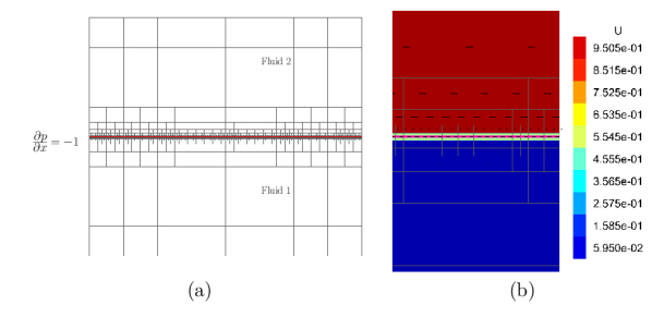
Figure 2: (a) Computational domain for the benchmark problem of Sec. IV.1 for parallel flow of Fluid 2 over Fluid 1 with a flat interface shown with a solid (red) line. The domain is 1$\times$1. The boundary conditions are prescribed pressures at inlet and outlet, and zero vertical pressure gradient at the top and bottom walls of computational domain. The interface is adaptively refined, with the smallest mesh size $\Delta=1/256$. (b) Computed velocities in Fluid 1, bottom, and Fluid 2, top; the viscosity ratio $\lambda=100$.

Consider two fluids of different viscosities in parallel flow. The Hele-Shaw equations (17)-(31) are solved for $\gamma=0$. The boundary conditions are: (i) prescribe pressures $p_{\text{in}}$ at the inlet and $p_{\text{out}}$ at the outlet such that a constant pressure difference $\Delta p=p_{\text{in}}-p_{\text{out}}$ is maintained; (ii) zero pressure gradient $\frac{\partial p}{\partial y}=0$ in the direction normal to the top and bottom boundaries; (iii) prescribe $f$ at the inlet, and zero gradient normal to the outlet $\frac{\partial f}{\partial x}=0$, to maintain parallel flow at the outlet (see Figure 2(a)).

The exact solution is a planar horizontal interface, with horizontal velocities

$$U_{i}=\frac{b^{2}}{12\mu_{i}}\frac{\Delta p}{L}.$$ (39)

The computations are performed for the following values: $\Delta p/\ell=1$, and the viscosity ratio $\lambda=\mu_{1}/\mu_{2}=100$, where subscripts 1 and 2 refer to the lower and upper fluids, respectively. Figure 2(b) shows the computed velocities. The solid (magenta) line shows the location of the interface, defined to be where the volume fraction of cells cut by the interface is 0.5. The computed velocities are shown in Figure 2(b), and agree with the exact solution in each fluid. At the interface, the exact slip velocity is

$$U_{1}-U_{2}=\frac{\mu_{2}-\mu_{1}}{\mu_{1}\mu_{2}}\frac{b^{2}}{12}\frac{\Delta p}{L}.$$ (40)

The computed slip velocity in cells that are cut by the interface is

$$U_{2}+f(U_{1}-U_{2}).$$ (41)

Note that the implementation of the weighted harmonic average for the viscosity, (28) and (30), achieves this exact slip velocity. On the other hand, if a naive ‘weighted mean’ average of the two viscosities is used to compute the viscosity of a mixed cell, and a simple average of cell center viscosities is used to interpolate the viscosity to the face of the cell, then the slip velocity of the mixed cell would be strongly shifted towards the more viscous fluid (Fluid 1 in this example). We avoid this inaccuracy.

IV.2 Circular interface in equilibrium: non-zero surface tension

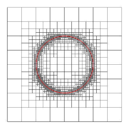
Figure 3: Benchmark computation from Sec. IV.2. Fluid 1 occupies the interior of the circle, and Fluid 2 occupies the exterior. The circular interface is shown as a solid (red ) line with radius 0.25, at the center of a 1$\times$1 computational domain. The interface is adaptively refined; here, the smallest mesh size $\Delta=1/128$.

Consider a circular drop placed at the center of a square computational domain that is initially at rest, as shown in Figure 3. The inflow and outflow boundary conditions are zero normal pressure gradients. The numerical simulation presented here is a test for the accuracy of the computation of the interfacial tension force. The initial configuration is a solution of (19) and satisfies the Young-Laplace condition, $[[p]]=\gamma\kappa$.

Table 1: Convergence results for the benchmark problem for Sec. IV.2. The norms $L_{1}$, $L_{2}$, and $L_{\infty}$ of the velocity, and the pressure jump across the interface are shown as a function of mesh refinement.

	$\Delta$=1/32	$\Delta$=1/64	$\Delta$=1/128
$L_{1}$	3.416e-06	5.686e-07	1.326e-07
$L_{2}$	5.234e-06	8.882e-07	2.083e-07
$L_{\infty}$	1.680e-05	2.879e-06	6.461e-07
$p_{1}-p_{2}$	4.03114	4.00750	4.00179

The computations are started at the discretized equilibrium solution, with zero velocity and a circular interface of radius $r=0.25$. The viscosity ratio is chosen as $\lambda=1$, the interfacial tension is $\gamma=1$, and the time step is $\Delta t=10^{-6}$. Table 1 presents the spatial convergence based on the $L_{1}$, $L_{2}$, and $L_{\infty}$ norms of the velocity field, and the pressure jump across the interface at the 5000th time step. ($p_{1}$ is the averaged pressure for cells with $r<0.25$ and $p_{2}$ is the averaged pressure for cells with $r>0.25$). It is clear that the velocity field decreases to zero with the mesh size ($\Delta=\frac{1}{32},\frac{1}{64},\frac{1}{128}$). At the 5000th time step, the computed velocity is not zero because the numerically computed interface shape has not reached an equilibrium. At each mesh resolution, there is a difference between the exact circular shape and the numerically computed interface shape; however, after a sufficient number of time steps, our balanced-force HF method has the feature of reaching the equilibrium velocity of zero to machine precision Afkhami and Bussmann (2009). At a fixed time step, the non-zero velocity diminishes at a second-order rate with mesh refinement. Additionally, the pressure jump across the interface approaches the exact value with second-order accuracy. Hence, Table 1 demonstrates that our numerical methodology for the interfacial tension force yields converged solutions.

IV.3 Translation of a viscous droplet in an unbounded Hele-Shaw flow

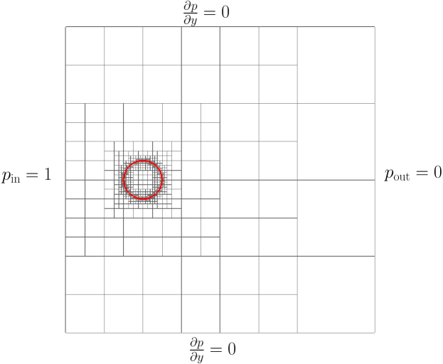
Figure 4: A droplet of Fluid 1, with a circular interface of radius 0.0625, is placed in a 1$\times$1 computational domain. The interface is shown as a solid (red) line. The domain is adaptively refined while the droplet translates in response to the flow of the surrounding Fluid 2.

Here we consider translational motion of a highly viscous droplet with high interfacial tension in an unbounded Hele-Shaw cell with an imposed uniform flow far from the droplet. The exact solution is the translation of the droplet. The fluid within the droplet moves as a rigid body with no recirculation. The boundary conditions for the pressure are: (i) at the upper and lower boundaries, the pressure gradient $\partial p/\partial y=0$; (ii) The pressure at the inlet is prescribed by the constant $p_{\text{in}}$ and at the outlet by the constant $p_{\text{out}}$ so that sufficiently far away from the drop, $\frac{\partial p}{\partial x}<0$. The boundary conditions for the VoF function are; (i) $f$ is prescribed to be Fluid 2 at the inlet and top and bottom walls, and $df/dx=0$ at the outlet. Computationally, the droplet must be much smaller than the cell to guarantee a constant pressure gradient far from the droplet.

We check the velocity of droplet translation. In this case it can be shown that a circle is an exact solution for the steady shape of the translating droplet of an arbitrary surface tensionGupta et al. (1999); Leshansky (2012) with the corresponding pressure distribution given in polar coordinates ($r,\theta$) by

$$p_{\text{drop}}=\left(\frac{2}{b}+\frac{1}{a}\right)\gamma+\frac{2\mu_{1}}{\mu_{1}+\mu_{2}}\frac{-\Delta p}{L}r\cos\theta,$$ (42)

$$p_{\text{matrix}}=\left(1+\frac{a^{2}}{r^{2}}\frac{\mu_{1}-\mu_{2}}{\mu_{1}+\mu_{2}}\right)\frac{-\Delta p}{L}r\cos\theta,$$ (43)

where $a$ is the droplet radius, $\theta$ is measured from the direction of the applied pressure gradient, and $r$ represents the radial distance from the center of the drop. The steady (rigid body) translational velocity of the circular drop is

$$U=\frac{b^{2}}{12\mu_{1}}\frac{2\mu_{1}}{\mu_{1}+\mu_{2}}\frac{\Delta p}{L}.$$ (44)

Table 2: The steady translational velocity of the circular drop for different viscosity ratios compared with the predicted velocity by (44).

	$\lambda=0.1$	$\lambda=1$	$\lambda=5$
$U_{\text{computed}}$	1.90	1.005	0.41
$U_{\text{theory}}$	1.82	1.0	0.33

Here we consider a drop of radius $0.0625$ placed in a 1$\times$1 computational domain. We check that the radius of the drop is small enough so that it will not affect the far field pressure distribution (Figure 4). We set $\gamma=1$, $\Delta p/\ell=1$, and vary the viscosity ratio $\lambda$ from $0.1$ to $5$. The comparison between the numerically computed steady translational velocity of the drop and (44) is shown in Table 2. We observe that the comparison is improved with better resolution of the flowfield. Figure 5 shows the snapshots of the numerical simulations for viscosity ratios of $0.1$, $1$, and $5$. More detail about the velocity and pressure fields follow.

First, it is evident that the initially circular drop (solid white line) remains in equilibrium for all cases. We also note that the translational velocity (44) does not depend on the interfacial tension; this is confirmed with numerical simulations at $\gamma=0.1$, $0.01$.

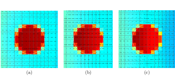
Figure 5: Linear pressure distribution and the velocity field for $\lambda=0.1$ (a), $1$ (b), and $5$ (c). Contours show the pressure field distribution with a maximum value colored in dark (red) and a minimum value colored in light (blue).

Secondly, Figure 5 shows the pressure distribution inside the drop (color contours). For $\lambda=1$, the pressure gradient inside the drop is simply $\partial p/\partial x=-\Delta p/\ell=-1$, in agreement with the theoretical value (42). This is the pressure gradient imposed at the far field. According to (42) for $\lambda=0.1$, the pressure gradient inside the drop is smaller and for $\lambda=5$, the pressure gradient inside the drop is larger than the imposed far field pressure gradient $\Delta p/\ell=1$. Figures 5(a)-5(c) support this prediction. It is also noted that the pressure distribution inside the drop for $\lambda=0.1$ is approximately a constant because it should be close to the pressure distribution of an inviscid drop ($\lambda\to 0$) in a Hele-Shaw cell which is known to have a steady translational velocity of 2. Thirdly, Figure 5 shows the velocity field inside and outside the drop. Clearly, each drop undergoes a rigid body translation with a steady velocity that is predicted by (44), i.e. the velocity inside the drop is a zero velocity field in a frame of reference moving with the drop steady-state velocity.

V Pressure driven flow of a co-flowing ribbon

We turn to the pressure-driven flow of a jet or ribbon of one fluid co-flowing with a second fluid which is shown in Figure 1, through a channel that is much wider than it is deep. For this flow, it is possible to make the jet form a tongue at the exit boundary, where the width of the tongue is extremely small. The production of small droplets, on the order of the depth of the channel, ensues in the reservoir, and is known as capillary focusing. Of practical importance is a simple estimate for the jet width $\delta$ at the exit; Ref. Malloggi et al., 2010 is a first attempt to estimate $\delta$ and compare with the experimental data. However, capillary focusing occurs at small capillary numbers, and the comparison appears to suffer in this regime, while the comparison for O(1) capillary number is satisfactory. Questions arise about the assumptions that are built into their estimate. This section clarifies this issue by directly interrogating the flow with numerical simulations.

V.1 A rough estimate for jet width at exit

A summary of the main assumptions in the prior estimateMalloggi et al. (2010) follows:

1. The $x$-component of the Hele-Shaw equation without the presence of the interface Ockendon and Ockendon (1995) is $\frac{12\mu}{b^{2}}V_{1}(x)=-\frac{\partial P(x,y)}{\partial x}$. This equation is integrated along two streamlines from the inflow to the outflow. Together with the outflow condition $P_{1}(0)=P_{2}(0)$, the result is $-P_{i}(-\infty)+P(0)=\frac{12\mu}{b^{2}}\int_{-\infty}^{0}V_{1}(x,y)dx$. The two streamlines are (i) along the centerline $y=0$ (Fluid 1), and (ii) at the wall $y=\frac{w}{2}$ (Fluid 2). Subtraction of one equation from the other yields

   $$-P_{2}(-\infty)+P_{1}(-\infty)=\frac{12}{b^{2}}\int_{-\infty}^{0}D(x)dx,$$

   $$D(x)=\mu_{2}U_{2}(x,\frac{w}{2})-\mu_{1}U_{1}(x,0).$$ (45)

   This relates the quantities at outflow to the prescribed inflow quantities, but in order to simplify this further, a decay property is imposed on $D(x)$.

2. At the interface between the fluids, the jump in the normal stress is balanced by surface tension effects. Here, because the depth $b$ is small, the in-plane curvature is neglected in comparison with the out-of-plane ($y$-$z$) value $\frac{2}{b}$, which originates from the semi-circular diameter. Hence, at inflow,

   $$\frac{2\gamma}{b}=P_{2}(-\infty)-P_{1}(-\infty).$$ (46)

   Substitution into (45) yields $\int_{-\infty}^{0}D(x)dx=\frac{-\gamma b}{6}$. Thus, the left hand side is a convergent improper integral. Therefore, the integrand must decay sufficiently fast to 0 at the lower end of the integration. This is taken one step further with the assumption that there is a decay length $\ell_{0}$, defined by $\int_{-\infty}^{0}D(x)dx=\ell_{0}D(0)$. This leads to a tractable expression

   $$\ell_{0}D(0)=\frac{-\gamma b}{6},\quad D(0)=\mu_{2}U_{2}(0)-\mu_{1}U_{1}(0).$$ (47)

   This and (45) are equations that link inflow (prescribed) and outflow (unknown) quantities.

3. Since the interior flow is not known a priori, a flux conservation is imposed

   $$U_{1\infty}w_{1\infty}=U_{1}(0)\delta,\quad U_{2\infty}w_{2\infty}=U_{2}(0)(w-\delta).$$ (48)

   Since $w_{i\infty}$ denotes the width of Fluid $i$ at inflow, we have $w_{1\infty}+w_{2\infty}=w$. Combined with (47), the unknown outflow velocities are eliminated and we have $D(0)$ in terms of the inflow data. Substitution in (46) gives the estimate for $\delta$. The final equation is $z^{2}\beta-z(1+Ca_{M})+Ca_{M}=0$, where

   $$\beta=\frac{w_{1\infty}}{w},\quad z=\frac{\delta}{w_{1\infty}}=\frac{\delta}{w\beta},$$ (49)

   and

   $$Ca_{M}=\mu_{2}\frac{6U_{2\infty}\ell_{0}}{b\gamma}=\mu_{1}\frac{6U_{1\infty}\ell_{0}}{b\gamma}.$$ (50)

   The equivalence of the two formulas follows from $D(-\infty)=0$. The usefulness of $Ca_{M}$ is limited because it depends on the unknown decay factor $\ell_{0}$. The estimate becomes

   $$z=\frac{(1+Ca_{M})}{2\beta}\left(1-\sqrt{1-\frac{4Ca_{M}\beta}{(1+Ca_{M})^{2}}}\right).$$ (51)

4. Some observations: (i) If the interfacial tension is large enough, then $Ca_{M}\ll 1$, and (51) predicts that $\delta$ decreases at the rate $z\sim Ca_{M}$. (ii) If the interfacial tension is small, then $Ca_{M}\gg 1$ and (51) predicts that $\delta$ is the same as the inflow width: $z\sim 1$. Indeed, any reasonable estimate must predict that the interface becomes flatter through the domain with increasing $Ca_{M}$. (iii) The free parameter $\ell_{0}$, set to $w/2$, is found to be a good fit to experimental data in Figure 2(c) of Ref. Malloggi et al., 2010.

V.2 Numerical simulations

Figure 6: The width of the jet $\delta$ upon exit scaled with $w_{1\infty}$ as a function of the capillary number $Ca$. $w/b=10$, $k=1$, and $w_{1\infty}/b=5$. Numerical results ($\small{\bullet}$) and an apparent fit (–) using (51) with $\ell_{0}/w=0.125$.

The flow conditions of Ref. Malloggi et al., 2010 are numerically simulated with $\mu_{1}=\mu_{2}$, and $dp_{1}/dx=dp_{2}/dx$ at the inflow. The exact solution which provides the inflow conditions is $w_{1\infty}/w=1/(1+k)$ where $k=(Q_{2\infty}\mu_{2})/(Q_{1\infty}\mu_{1})$, and the flow rates $Q_{i\infty}$ for $i=1$, $2$ are defined in (24). Our capillary number is defined by

$$Ca=\frac{\mu_{1}U_{1\infty}}{\gamma},$$ (52)

and is not $Ca_{M}$ in (50). The channel aspect ratio $w/b$ is assumed large, and the Hele-Shaw approximation is expected to be more accurate as $w/b$ increases. Figure 6 reports the results of the numerical simulations ($\small{\bullet}$) for $\delta$ as a function of the capillary number $Ca$ for $w/b=10$, $k=1$, and $w_{1\infty}/b=5$, together with an apparent fit (–) using (51), with $\ell_{0}/w=0.125$. Note that the interface remains straight when the interfacial tension is small; this accounts for $\delta/w_{1\infty}\approx 1$ when $Ca$ is large. This is also found in Figure 2(c) of Ref. Malloggi et al., 2010, where the trend at $Ca=O(1)$ is used to choose $\ell_{0}/w$. The problem with this method is that on the scale of the figure, the results for $Ca\ll 1$ are too small to be discerned. The line in Figure 6 represents the estimate (51) with a choice of $\ell_{0}/w=0.125$, and shows an apparent fit. However, the jet forms a tongue only if $Ca\ll 1$, and we next focus on this regime.

Figure 7: Steady-state jet solution for $Ca=0.01$, $0.025$, $0.05$, $0.1$, and $0.2$ (small to large $\delta$), for $w/b=10$, $k=1$, and $w_{1\infty}/b=5$. The curvature at the outlet is $\kappa=2/b$.

Figure 7 shows the numerically computed steady-state shapes of the jet for $w/b=10$, $k=1$, and $w_{1\infty}/b=5$. The capillary number is varied from $0.01$ to $0.2$ in order to show the same trend as in the available experimental data: the jet narrows more at the outlet as the capillary number decreases Priest, Herminghaus, and Seemann (2006); Malloggi et al. (2010).

Figure 8: Relative error $E(z)$ of (51) as a function of $Ca$ for $\ell_{0}/w=0.5$ ($\bullet$) and $0.125$ ($\small{\blacktriangle}$).

It is informative to present the relative error of the model $z_{m}$ (51) with respect to the exact computed values $z_{c}$, defined by

$$E(z)=\frac{z_{c}-z_{m}}{z_{c}}.$$

Figure 8 shows $E(z)$ as a function of $Ca$. If $Ca$ increases past $0.1$, then the interfacial tension is weak and the interface tends to stay undeformed; $\delta/w_{1\infty}$ naturally approaches 1, no matter the choice of $\ell_{0}/w=0.5$ ($\bullet$) and 0.125 ($\small{\blacktriangle}$). However, if $Ca$ is small, then Figure 8 shows that the relative errors are large no matter what value of $\ell_{0}/w$ is picked. Therefore, the assumption in Sec. V.1 that the decay length $\ell_{0}$ is comparable to the channel width $w$ is not correct. With hindsight, we see that the assumption of such a large decay region is incompatible with the assumption in Sec. V.1 that the velocity is uniform in each fluid along $x=$ constant, and also with the assumption that the $y$-component of velocity has no role in the derivation of (51). The numerical simulations also confirm the expectation that there is a significant $y$-component of velocity in a much smaller ‘decay region’ very close to the exit.

Figure 9: (a) $U_{1}(0)$ and (b) $U_{2}(0)$, normalized by $U_{1\infty}$ and $U_{2\infty}$, respectively, along the outflow boundary $x=0$. $Ca=0.05$, $w_{1\infty}/b=5$, and $w/b=10$. $\mu_{1}/\mu_{2}=1$. $k=1$.

Figure 9 confirms that the flux does not satisfy the assumption (48), which feeds into (51). The figure shows numerically computed velocities $U_{1}(0)$ and $U_{2}(0)$ (here we use $x=0$ to denote the outflow position and $x=-\infty$ for inflow), normalized by $U_{1\infty}$ and $U_{2\infty}$, respectively, along the outflow boundary. The numerical results show a complex non-uniform velocity field at outflow, which is ignored if only the inflow and outflow flux conditions are used in the theoretical analysis. An interesting feature of the velocity distribution in Figure 9 is a strong slip between the inner and outer fluids. There is more than an order of magnitude difference between the inner phase and outer phase velocity at the Fluid 1-Fluid 2 interface. The corresponding velocity field is shown in Figure 10. The square cells depicted in Fluid 1 illustrate the spatial discretization for the adaptive mesh refinement. The shading indicates the pressure distribution. The numerical results of Figures 9 and 10 are for $Ca=0.05$ where the flow focusing is moderate compared with the stronger focusing at smaller values of $Ca$ shown in Figure 7. On the other hand, if $Ca$ is larger than 0.1, we find that the assumption of gentle flow variation from inflow to outflow, which was used to obtain (51), is reasonable.

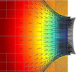
Figure 10: Flow field and the pressure distribution in the focusing region for $Ca=0.05$, $w_{1\infty}/b=5$, and $w/b=10$; $\mu_{1}/\mu_{2}=1$ and $k=1$. The pressure contours show that at the outflow boundary, the pressures in both phases equilibrate.

Figure 11 shows the numerical results of the steady-state shapes of the interface at three values of the capillary number, and confirms that the focusing effect is stronger for smaller capillary numbers. The significant focusing is evident at $Ca=0.016$ (Figure 11(a)); i.e. high surface tension yields improved self-focusing. Figure 11 also shows an important feature that by decreasing the channel depth, the narrow jet develops a sharp tip at the outflow boundary. The pressure distributions are shown in Figure 11 for varying $Ca$ and $w/b$.

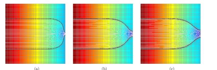
Figure 11: Effect of surface tension and channel depth on self-focusing. Contours depict the pressure field distribution with a maximum value colored in dark (red) and a minimum value colored in light (blue). The adaptive mesh and the streamlines in the inner stream are also shown. (a) $Ca=0.016$, $w_{1\infty}/b=10$, and $w/b=20$. (b) $Ca=0.033$, $w_{1\infty}/b=5$, and $w/b=10$. (c) $Ca=0.052$, $w_{1\infty}/b=3.33$, and $w/b$=6.66. $\mu_{1}/\mu_{2}=1$ and $k=1$.

Figure 12: Interface profiles. (a) $w_{1\infty}/b=10$, 5, and 3.33 (top to bottom profiles); $Ca=0.033$. (b) $Ca$=0.05, 0.033, and 0.025 (top to bottom profiles); $w_{1\infty}/b=5$, and $w/b=10$. $\mu_{1}/\mu_{2}=1$ and $k=1$. Only half of the computational domain is shown.

To show the effect of the flow rate of the inner phase on the narrowing of the tip, interface profiles are shown in Figure 12(a) when varying $w_{1\infty}/b$. The main feature is that increasing the flow rate of the inner phase results in an abrupt change in the interface curvature, i.e. the length over which the deformation of the interface takes place decreases. If the flow rate of the inner phase is small, then the change in the interface curvature is more gentle. However, in this scenario, the Hele-Shaw approximation breaks down because $\delta<b$. This may be the contributing factor for the different breakup mechanisms reported in Ref. Priest, Herminghaus, and Seemann, 2006 when changing the flow rate of the inner phase from low to high.

In Figure 12(b), $w_{1\infty}/b$ and $w/b$ are kept constant while varying $Ca$. Figure 12(b) shows that the characteristic length over which the abrupt change of the interface curvature occurs is weakly dependent on $Ca$ once the capillary number is below a critical value.

To demonstrate the local change of the interface shape in the focusing region, the computed interface curvature is shown in Figure 13 for $Ca=0.03$, $0.1$, and $0.3$. This shows the abrupt change in the narrowing region, where the curvature changes sign from being $-2/b$ at the outflow to zero at inflow. (Note that with $p=0$ at the outflow boundary, we arrive at $\kappa=-2/b$ at the outlet $x=0$.) As shown, the increase in the capillary number results in the decrease of the length scale over which the curvature changes sign.

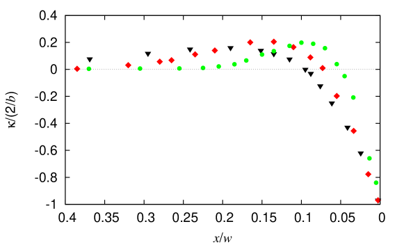
Figure 13: Computed interface curvature normalized by $2/b$, the magnitude of the curvature at the outflow ($x=0$), as a function of $x/w$ for $Ca=0.03$ ($\blacktriangledown$), $0.1$ ($\blacklozenge$), and $0.3$ ($\bullet$); the dashed line, $\kappa=0$, is only plotted to guide the eye. $w_{1\infty}/b=5$, and $w/b=10$; $\mu_{1}/\mu_{2}=1$ and $k=1$.

VI Conclusions

The formulation and implementation of a robust volume-of-fluid height-function numerical algorithm for the Hele-Shaw equations with two immiscible liquids are presented. The components of the numerical scheme are validated with benchmark computations. The simulation of a ribbon of fluid which co-flows with a second liquid through a Hele-Shaw cell is carried out to give a critical assessment of the theory of Ref. Malloggi et al., 2010 for an estimate of the jet width at exit. The parameters in the numerical simulations are taken from the controlled experiments in the literature Priest, Herminghaus, and Seemann (2006); Malloggi et al. (2010). The results show that when the capillary number is small, there is a region just short of the exit where the flowfield changes in a complex manner, and which is not captured by simply looking at the inflow and outflow fluxes. An example is the sign reversal in curvature at the exit, which is clearly seen in the numerical simulations. We also find that the effect of increasing the jet phase flow rate is to encourage the abrupt change in the interface curvature.