Searching for the core variables in principal components analysis

Abstract

In this article, we introduce a procedure for selecting variables in principal components analysis. It is developed to identify a small subset of the original variables that best explain the principal components through nonparametric relationships. There are usually some noisy uninformative variables in a dataset, and some variables that are strongly related to one another because of their general dependence. The procedure is designed to be used following the satisfactory initial principal components analysis with all variables, and its aim is to help to interpret the underlying structures. We analyze the asymptotic behavior of the method and provide some examples.

arXiv:1308.6626

, and

a]Universidad de San Andrés and CONICET

1 Introduction

Principal components analysis (PCA) is the best known dimensional reduction procedure for multivariate data. An important drawback of PCA is that it sometimes provides poor quality interpretation of data for practical problems, because the final output is a linear combination of the original variables. The aim of the present study is to identify a small subset of the original variables in a dataset, whilst retaining most of the information related to the first $k$ principal components.

There is a large body of literature that focuses on trying to interpret principal components. Jolliffe (1995) has introduced rotation techniques. Vines (2000) proposed to restrict the value of the loadings for PCA to a small set of allowable integers such as {-1, 0, 1}. McCabe (1984) presented a different strategy that aims to select a subset of the original variables with a similar criterion to PCA.

A few years later a whole literature of variable selection appeared, inspired by the LASSO (least absolute shrinkage and selection operator). This technique was introduced by Tibshirani (1996). The way the LASSO works was described thus: “ It shrinks some coefficients and sets others to 0, and hence tries to retain the good features of both subset selection and ridge regression… The ‘LASSO’ minimizes the residual sum of squares subject to the sum of the absolute value of the coefficients being less than a constant. Because of the nature of this constraint it tends to produce some coefficients that are exactly 0 and hence gives interpretable models.”

Jolliffe et al. (2003) proposed SCoTLASS that imposes a bound on the sum of the absolute values of the loadings in the component, using a similar idea to the one that LASSO used in regression. Zou et al. (2006) presented SPCA (sparse PCA) that extends the “elastic net” of Zou & Hastie (2005) that was a generalization of the LASSO. As they mentioned “SPCA is built on the fact that PCA can be written as a regression-type optimization problem, with quadratic penalty; the LASSO penalty (via the elastic net) can then be directly integrated into the regression criterion, leading to a modified PCA with sparse loadings.”

Luss & d’Aspremont (2010) studied the application of sparse PCA to clustering and problems of feature selection. Sparse PCA seeks sparse factors, or linear combinations of variables in the dataset, to explain as much variance in the data as possible while limiting the number of nonzero coefficients as far as possible. The authors applied their results to some classic biological clustering and feature selection problems.

Recently, Witten & Tibshirani (2008) introduced the notion of Lassoed principal components for identifying differentially-expressed genes, and considered the problem of testing the significance of features in high dimensional data.

Our approach is rather different and is designed to be used after satisfactory PCA has been achieved rather than, as in other methods, to produce principal components with particular characteristics (e.g., some coefficients that are zero) so that only interpretable principal components are produced. We first perform classical PCA and then look for a small subset of the original variables that contain almost all the relevant information to explain the principal components. However, our method can also be used after performing any sparse PCA method as those described previously.

To develop our method, we borrowed some ideas for selecting variables from Fraiman et al. (2008), who introduced two procedures for selecting variables in cluster analysis, and classification rules. Both of these procedures are based on the idea of “blinding” unnecessary variables. To cancel the effect of a variable, they substituted all its values with the marginal mean (in the first procedure) or with the conditional mean (in the second). The marginal mean approach was mainly intended to identify “noisy” uninformative variables, but the conditional mean approach could also deal with dependence. We adapted the idea behind the second procedure to PCA.

In Section 2, we introduce the main definitions, a population version of our proposed method, and the empirical version; we also present our main results. In Section 3, a simulation study is conducted, where the results are compared with other well-known PCA variable selection procedures. Finally, in Section 4, we study a real data example. Proofs are given in the Appendix.

2 Our method: Definitions and properties

We begin by defining our notation and stating the problem in terms of the underlying distribution of the random vector $\mathbf{X}$. Then we give our estimates based on the sample data, via the empirical distribution.

2.1 Population version

We define $\mathbf{X}\in\mathbb{R}^{p}$ as a random vector with distribution $\mathbb{P}$. The coordinates of the vector $\mathbf{X}$ are defined as $X[i],\ \ i=1,\ldots,p$. The covariance matrix of $\mathbf{X}$ is denoted $\Sigma$.

For a given random vector $\mathbf{\tilde{X}}$, we say that it satisfy the Assumption H1 if:

• $\mathbb{E}(\|\mathbf{\tilde{X}}\|^{2})<\infty$;

• The covariance matrix of $\mathbf{\tilde{X}}$ is positive definite.

• All the eigenvalues of the covariance matrix are different.

Throughout the manuscript, $\mathbf{X}$ fulfills Assumption H1.

As is well known, the first principal component associated with the vector $\mathbf{X}$ is defined as

$$\alpha^{1}(\mathbb{P}):=\alpha^{1} = \underset{\left\|\alpha\right\|=1}{arg\ max}\ Var\left(\mathbf{\alpha^{\prime}}\mathbf{X}\right)$$

$$= \underset{\left\|\mathbf{\alpha}\right\|=1}{arg\ max}\ \mathbf{\alpha}^{\prime}\Sigma\mathbf{\alpha},$$

and the next principal components are defined as

$$\alpha^{k}(\mathbb{P}):=\alpha^{k} = \underset{\left\|\mathbf{\alpha}\right\|=1,\ \mathbf{\alpha}\bot[\alpha^{1},\ldots,\alpha^{k-1}]}{arg\ max}\ Var\left(\mathbf{\alpha}^{\prime}\mathbf{X}\right)$$

$$= \underset{\left\|\mathbf{\alpha}\right\|=1,\ \mathbf{\alpha}\bot[\alpha^{1},\ldots,\alpha^{k-1}]}{arg\ max}\ \mathbf{\alpha}^{\prime}\Sigma\mathbf{\alpha}\ \ \forall\ 2\leq k\leq p,$$

where $[\alpha^{1},\ldots,\alpha^{k-1}]$ is the subspace generated by the vectors $\{\alpha^{1},\ldots,\alpha^{k-1}\}$.

From the spectral theorem, it follows that, if $\lambda^{1}>\lambda^{2}>\ldots>\lambda^{p}$ are the $\Sigma$ eigenvalues, the solutions to the PCA are the corresponding eigenvectors, $\alpha^{k},\ \ k=1,\ldots,p$.

Given a subset of indices $I\subset\{1,\ldots,p\}$ with cardinality $d\leq p$, we define $\mathbf{X}[I]$ as the subset of random variables $\{X[i],i\in I\}$. With a slight abuse of notation, if $I=\{i_{1}<\ldots<i_{d}\}$, we can also denote $\mathbf{X}[I]$ to the vector $(X[i_{1}],\ldots,X[i_{d}])$, and define the vector $\mathbf{Y}^{I}:=(Y^{I}[1],\ldots,Y^{I}[p])$, where

$$Y^{I}[i]=\left\{\begin{array}[]{ccc}X[i]&&\text{ if }i\in I\\ \mathbb{E}(X[i]|\mathbf{X}[I])&&\text{ if }i\notin I.\end{array}\right.$$

$\mathbf{Y}^{I}\in\mathbb{R}^{p}$ depends only on the $\{X[i],i\in I\}$ variables and then the principal components associated with the vector $\mathbf{Y}^{I}$ depend only on the variables in $\mathbf{X}[I]$. The distribution of $\mathbf{Y}^{I}$ is denoted $\mathbb{P}_{\mathbf{Y}^{I}}$, the covariance matrix is $\Sigma_{\mathbf{Y}^{I}}$ and $g^{i}(z)=\mathbb{E}(X[i]|\mathbf{X}[I]=z)$ for $i\notin I$ is the regression function.

In what follows we assume that $\mathbf{Y}^{I}$ fulfills the Assumption H1.

Remark: This assumptions will not hold if there is a variable $X[i]$ such that $g^{i}(z)$ is a linear combination of the variables in $I$. For instance, if $\mathbf{X}$ is gaussian or $X[i]$ is independent of the variables in $I$. In practice we will see how this problem can be tackled in the example 2 of section 3.

We are looking for a subset $I$ of small cardinality that minimizes the distance between the original principal components and the principal components that are function of the variables in the subset $I$. This can be done following two different approaches.

Local approach

We define the objective function $h^{1}(I)$ as

$$h^{1}(I,\mathbb{P},\mathbb{P}_{\mathbf{Y}^{I}}):=h^{1}(I,\mathbb{P}):=h^{1}(I)=\|\alpha^{1}(\mathbb{P})-\alpha^{1}(\mathbb{P}_{\mathbf{Y}^{I}})\|^{2},$$ (2.1)

which measures the squared distance between the first original principal component and the first principal component that is a function of the variables in the subset $I$.

Given a fixed integer $d$, $1\leq d<<p$, $\mathcal{I}_{d}$ is the family of all subsets of $\{1,\ldots,p\}$ with cardinality $d$ and $\mathcal{I}_{1,0}\subset\mathcal{I}_{d}$ is the family of subsets in which the minimum $h^{1}(I)$ is attained for $I\in\mathcal{I}_{d}$, i.e.,

$$\mathcal{I}_{1,0}=argmin_{I\in\mathcal{I}_{d}}h^{1}(I),$$

or, equivalently,

$$h^{1}(I_{1})=min_{I\in\mathcal{I}_{d}}h^{1}(I)\text{ for all }I_{1}\in\mathcal{I}_{1,0}.$$ (2.2)

Analogously, we define

$$h^{k}(I,\mathbb{P},\mathbb{P}_{\mathbf{Y}^{I}}):=h^{k}(I,\mathbb{P}):=h^{k}(I)=\|\alpha^{k}(\mathbb{P})-\alpha^{k}(\mathbb{P}_{\mathbf{Y}^{I}})\|^{2},$$ (2.3)

and

$$\mathcal{I}_{k,0}=argmin_{I\in\mathcal{I}_{d}}h^{k}(I),$$

for $k=2,\ldots,p$.

For $k=1,\ldots,p$ (2.3) measures the squared distance between the $k$-th original principal component and the $k$-th principal component that is a function of the variables in the subset $I$.

Principal components may, in some cases, be rather difficult to interpret, which is an important issue in practice. If we can find a small cardinal subset $I$, for which the objective function (2.3) is small enough, then the $k$-th principal component will be well explained by a subset of the original variables.

Global approach

In this case, the objective function is

$$h(I):=\sum_{k=1}^{q}p_{k}h^{k}(I),$$ (2.4)

with $p_{k}\geq 0,\ \sum_{k=1}^{q}p_{k}=1,\ 2\leq q<p$,
and we define

$$\tilde{\mathcal{I}}_{q,0}=argmin_{I\in\mathcal{I}_{d}}h(I).$$

This time the objective function (2.4) deals with finding a unique subset $I$ to explain the first $q$ principal components at once. If we think that the $q$ components are equally important then we choose $p_{k}=\frac{1}{q}$. Otherwise, if some components are more important than others then we can put different weights. As a default we suggest choosing weights proportional to the variance that each component is explaining, i.e. $p_{k}=\lambda^{k}/\sum_{k=1}^{q}\lambda^{k}$.

On the Local approach, we consider a different subset for each principal component, using the objective function (2.3) for each $k$. On the Global approach, we seek a unique subset for all the first $q$ principal components using (2.4). In practice, we can choose $q$, so that the first $q$ principal components explain a high percent of the total variance and consider a subset for this principal components.

These subsets tell us which are the original variables that “best explain” the first $q$ principal components. In what follows we refer to this method as the Blinding Procedure (BP).

An important issue is how to choose $d$, the cardinality of the set $I$. On the one hand we have that the objective function (2.3) decreases when $d$ increases for every $k$. On the other hand we look for a subset $I$ with small cardinality, so we have a constant tug of war. Since the components have unitary norms there is a direct relationship between (2.3) and the angle between the two vectors. It is clear that the smaller the angle is the closer the components are.

Hence, for the $k$-th component we propose to fix an angle, $\gamma$, and choose $d$ as the smallest value for which $\mathcal{I}_{k,0}(d)$ makes the angle between the blinding and the original component smaller than $\gamma$.

If we want “to explain” the first $q$ principal components at once, we propose to fix an angle, $\gamma$, and choose $d$ as the smallest value for which $\tilde{\mathcal{I}}_{q,0}(d)$ makes the largest of the $q$ angles smaller than $\gamma$. In both cases, the angle $\gamma$ must be chosen by the user. As default, we propose to fix an angle not larger than 25 degrees.

2.2 Empirical version. Consistent estimates of the optimal subset

We aimed to consistently estimate the sets $I_{1},\ldots,I_{q}$ from a sample $\textbf{X}_{1},\ldots,\mathbf{X}_{n}$ of i.i.d. random vectors with distribution $\mathbb{P}$.

Given a subset $I\in\mathcal{I}_{d}$, the first step is to build a sample $\mathbf{Y}_{1}^{I},\ldots,\mathbf{Y}_{n}^{I}$ of random vectors in $\mathbb{R}^{p}$, which only depends on $\mathbf{X}[I]$, using nonparametric estimates of the conditional expectation (the regression function). Below, we assume that

Assumption H2 For all $i\notin I$, $g^{i}_{n}(z)$ is a strongly consistent estimate of $g^{i}(z)$ uniformly in $z$. Conditions under which H2 holds can be found in Hansen (2008).

First, we define the empirical version of the blinded observations. As an example, we consider the nearest neighbours estimator. We therefore set an integer value $r$ (the number of nearest neighbours that we are going to use) with respect to an appropriate metric (typically Euclidean or Mahalanobis distance), only considering the coordinates on $I$.

More precisely, for each $j\in\{1,\ldots,n\}$, we find the set of indices $C_{j}=:C_{j}(X_{j}[I])$ of the $r$-nearest neighbours of $\mathbf{X}_{j}[I]$ among $\{\mathbf{X}_{1}[I],\ldots,\mathbf{X}_{n}[I]\}$, where $\mathbf{X}_{j}[I]=\{X_{j}[i],i\in I\}$.

Next, we define the random vectors $\mathbf{Y}_{j}^{I},1\leq j\leq n$, verifying:

$$Y_{j}^{I}[i]=\left\{\begin{array}[]{ccc}X_{j}[i]&&\text{ if }i\in I\\ \frac{1}{r}\sum_{m\in C_{j}}X_{m}[i]&&\text{ otherwise,}\end{array}\right.$$ (2.7)

where $X_{j}[i]$ stands for the ith-coordinate of the vector $\mathbf{X}_{j}$.

This corresponds to use for $i\notin I$ the nonparametric estimate

$$g^{i}_{n}(z)=g^{i}_{n}(z[I])=\frac{1}{r}\sum_{m\in C_{j}(z[I])}X_{m}[i],$$

since $g^{i}_{n}(z)$ is a strongly consistent estimate of $g^{i}(z)$, where $g^{i}(z)=\mathbb{E}(X[i]|\mathbf{X}[I]=z)$. Moreover, observe that the notation $z[I]$ is to emphasize that the function depends on the coordinates indicated by the subset $I$.

$\mathbb{P}_{n}$ stands for the empirical distribution associated with $\{\mathbf{X}_{j},1\leq j\leq n\}$ and $\mathbb{P}_{n,\mathbf{Y}^{I}}$ stands for the empirical distribution of $\{\mathbf{Y}_{j}^{I},1\leq j\leq n\}$.

In our examples to consistently estimate the optimal number of nearest neighbours we use the generalized cross validation procedure proposed by Li & Gong (1987), i.e.

$$\widehat{r}_{opt}(i,I)=\arg\min_{r}\frac{\frac{1}{n}\sum_{j=1}^{n}\left(X_{j}[i]-Y_{j}[i]\right)^{2}}{\left(1-\frac{1}{r}\right)^{2}},\quad i\notin I.$$

When $d$ is large, nonparametric estimators perform poorly due to the curse of dimensionality. In this case, a semi-parametric approach should be used like that proposed by He & Shi (1996). Also a recent proposal by Biau et al. (2013) called COBRA can be used to avoid the curse of dimensionality. The consistency result given in the following theorem will still be valid as long as the semi-parametric estimates verify the consistency assumptions required for the purely nonparametric estimates.

We will be mainly interested in cases where $d$ is small. In our experience a good idea is to start the search with some genetic algorithm which provides an initial solution with a few variables ($d$ small) and then improve the result working with $card(I)\leq d$. Also a forward-backward algorithm as the one proposed in Fraiman et al. (2008) can be used.

Finally, we define, for each $I\in\mathcal{I}_{d}$, the corresponding empirical versions

$$\hat{\mathbf{\alpha}}^{k}_{n}(I):=\alpha^{k}(\mathbb{P}_{n,\mathbf{Y}^{I}}),\hat{h}^{k}_{n}(I)=h^{k}(I,\mathbb{P}_{n},\mathbb{P}_{n,\mathbf{Y}^{I}}),\hat{I}_{kn}=argmin_{I\in\mathcal{I}_{d}}\hat{h}^{k}_{n}(I)$$ (2.8)

and

$$\hat{h}_{n}(I)=\sum_{k=1}^{q}p_{k}\hat{h}_{n}^{k}(I),\ \ \hat{I}_{n}=argmin_{I\in\mathcal{I}_{d}}\hat{h}_{n}(I)$$ (2.9)

respectively.

Let us observe that $\hat{\mathbf{\alpha}}^{k}_{n}(I)$ corresponds to the principal component associated with the sample $\{\mathbf{Y}_{j}^{I},1\leq j\leq n\}$. $\hat{h}^{k}_{n}(I)$ corresponds to the objective function of the k-th principal component, it measures the square distance between the k-th original principal component and the k-th principal component that is a function of the variables in the subset $I$. The function $\hat{h}^{k}_{n}(I)$ determines which are the variables that retain most of the information related to the k-th principal component. The variables we are choosing are the ones that minimize the function $\hat{h}^{k}_{n}(I)$. The subset $\hat{I}_{kn}$ indicates which this variables are. In case we are looking for a unique subset $I$ to explain the first $q$ principal components, we consider the function $\hat{h}_{n}(I)$.

A robust version can be obtained using robust principal components (see for instance Maronna et al. (2006)) and replacing in (2.7) the local mean by local median.

Theorem 2.1.

Under assumptions H1 for $\mathbf{X}$ and $\mathbf{Y}^{I}$ and H2 we have that $\hat{I}_{kn}\in\mathcal{I}_{k,0}$ ultimately for $k=1,\ldots,q$, i.e., $\hat{I}_{kn}=I_{k}$ with $I_{k}\in\mathcal{I}_{k,0}$ $\forall n>n_{0}(\omega)$, with probability one. We also have that $\hat{I}_{n}\in\mathcal{\tilde{I}}_{q,0}$ ultimately.

Proof.

The proof is given in the Appendix. ∎

3 Some simulated examples

In this section we consider two simulated experiments to analyze the behavior of our method and compare it with other methods proposed in the literature.

3.1 Example 1

To better understand the heart of our procedure we start with a simple simulation example in dimension four.

There are two “hidden” factors:

$$V_{1}\sim N(0,1.25^{2}),$$

$$V_{2}\sim N(0,0.55^{2}),$$

where $V_{1}$, $V_{2}$ are independent.

We construct the 4 observable variables as follows:

$$X_{1}=V_{1}+\epsilon_{1},$$ (3.1)

$$X_{2}=|V_{1}|+\epsilon_{2},$$

$$X_{3}=V_{2}+\epsilon_{3},$$

$$X_{4}=V_{1}V_{2}+\epsilon_{4},$$

where $\varepsilon_{j}$, $1\leq j\leq 4$ are i.i.d. $N(0,\sigma^{2})$, with $\sigma=0.01$ (Case 1), $\sigma=0.1$ (Case 2) and $\sigma=0.25$ (Case 3).

When we perform the variable selection it is clear that two variables containing the information given by $V_{1}$ and $V_{2}$ should be kept. This means that $\{X_{1},X_{3}\}$, $\{X_{1},X_{4}\}$ or $\{X_{3},X_{4}\}$ would be “good” choices while $\{X_{1},X_{2}\}$ is clearly a “bad” choice since only retains information of $V_{1}$. Additionally, $\{X_{2},X_{3}\}$ (respec. $\{X_{2},X_{4}\}$) is not a “good” choice since can not recover all the information of $V_{1}$ (respec. $V_{1}$ and $V_{2}$).

In this example, in all the cases, we compare our procedure with other proposals: algorithms $B2$ and $B4$ (Jolliffe (2002)), a variable selection approach proposed by McCabe (1984) and sparce PCA introduced by Zou et al. (2006). To retain $q$ variables, algorithm $B2$ associates one of the original variables to each of the $p-q$ last PCA vectors and deletes those variables, while $B4$ associates one of the original variables to each of the first $q$ PCA vectors and retains those variables.

For each case, we perform 500 replicates and on each of them we generate samples of size 100 from model (3.1) and compute the covariance matrix.

• Case 1: The first two principal components explain between 70 and 85 percent of the total variance. For the BP 85% of the times the maximum angle conformed by the first two principal components is smaller than 25 degrees, hence we keep two variables.
  The results exhibitted in Table 1 on page  1 show that 78% of the times the BP makes a “good” choice of variables, $B2$ only does it 27% of the times, while the other methods fail in more than 75% of the replications.

  Table 1: Proportion of times where each method selects each pair of variables.(Case 1)

  	BP	B2	B4	McCabe	SPCA
  $X_{1},X_{2}$	$0.22$	$0.732$	$0.76$	$0.782$	$0.76$
  $X_{1},X_{3}$	$0.37$	$0.004$	$0.002$	$0.002$	$0.002$
  $X_{1},X_{4}$	$0.366$	$0.264$	$0.238$	$0.216$	$0.238$
  $X_{2},X_{3}$	$0$	$0$	$0$	$0$	$0$
  $X_{2},X_{4}$	$0$	$0$	$0$	$0$	$0$
  $X_{3},X_{4}$	$0.044$	$0$	$0$	$0$	$0$

• Case 2: The first two principal components explain between 69 and 85 percent of the total variance. For the BP more than 78% of the times the maximum angle conformed by the first two principal components is smaller than 25 degrees, hence we keep two variables.
  The results exhibitted in Table 2 on page  2 show that that 75% of the times the BP makes a “good” choice of variables, $B2$ only does it 29% of the times, $B4$ and SPCA 27%, while McCabe fails in more than 75% of the replications.

  Table 2: Proportion of times where each method selects each pair of variables.(Case 2)

  	BP	B2	B4	McCabe	SPCA
  $X_{1},X_{2}$	$0.248$	$0.714$	$0.728$	$0.752$	$0.728$
  $X_{1},X_{3}$	$0.354$	$0.002$	$0.002$	$0.002$	$0.002$
  $X_{1},X_{4}$	$0.368$	$0.284$	$0.27$	$0.246$	$0.27$
  $X_{2},X_{3}$	$0$	$0$	$0$	$0$	$0$
  $X_{2},X_{4}$	$0$	$0$	$0$	$0$	$0$
  $X_{3},X_{4}$	$0.03$	$0$	$0$	$0$	$0$

• Case 3: The first two principal components explain between 67 and 82 percent of the total variance. For the BP,  69% of the times the maximum angle conformed by the first two principal components is smaller than 25 degrees, hence we keep two variables.
  The results exhibitted in Table 3 on page  3 show that 74% of the times the BP makes a “good” choice of variables, $B2$ does it 51% of the times, $B4$ and SPCA 48%, while McCabe 46%.

  Table 3: Proportion of times where each method selects each pair of variables.(Case 3)

  	BP	B2	B4	McCabe	SPCA
  $X_{1},X_{2}$	$0.264$	$0.488$	$0.516$	$0.536$	$0.516$
  $X_{1},X_{3}$	$0.192$	$0.002$	$0$	$0$	$0$
  $X_{1},X_{4}$	$0.54$	$0.51$	$0.484$	$0.464$	$0.484$
  $X_{2},X_{3}$	$0$	$0$	$0$	$0$	$0$
  $X_{2},X_{4}$	$0$	$0$	$0$	$0$	$0$
  $X_{3},X_{4}$	$0.004$	$0$	$0$	$0$	$0$

From the definition of $X_{1}$ and $X_{2}$ we have that $X_{2}$ is a function of $X_{1}$ plus an error. We can see from Table 1 on page  1, Table 2 on page  2 and Table 3 on page  3 that our procedure selects $X_{1}$ and $X_{2}$ only between 0.22 and 0.264 proportion of the times, when the other procedures select it in around a 0.5 proportion of the times or more. In most of the cases our procedure detects that $X_{2}$ is a “function” of $X_{1}$. That is, if $X_{1}$ is selected to be one of the two explanatory variables, for the other one, the BP, select between $X_{3}$ and $X_{4}$. This way, the BP gains information about $V_{2}$ instead of getting redundant information by choosing $X_{2}$. Note that $\{X_{3},X_{4}\}$ is also a “good” choice.

To make the problem a bit more challenging we enlarge the dimension of the dataset repeating the same variables plus noisy noninformative errors and also add some i.i.d. noisy variables. More precisely we consider the following model:

$$X_{j}=\left\{\begin{array}[]{ccccc}V_{1}+\varepsilon_{j},&&\text{ if }1\leq j\leq 5,\\ |V_{1}|+\varepsilon_{j},&&\text{ if }6\leq j\leq 10,\\ V_{2}+\varepsilon_{j},&&\text{ if }11\leq j\leq 15,\\ V_{1}V_{2}+\varepsilon_{j},&&\text{ if }16\leq j\leq 20,\\ \varepsilon_{j},&&\text{ if }21\leq j\leq 23,\end{array}\right.$$

where $\varepsilon_{j}$, $1\leq j\leq 23$ are i.i.d. $N(0,\sigma^{2})$, with $\sigma=0.01$ (Case 1), $\sigma=0.1$ (Case 2) and $\sigma=0.25$ (Case 3).

We keep the first and second principal component because on 98% of the 500 replicates they explain between 70% and 85% of the total variance in Case 1, between 70% and 83% in Case 2 and between 65% and 78% in Case 3. Again we require all the methods to select two variables. In the three cases, at least 93% of the times the largest angle is smaller than 25 degrees, hence we consider it is a good decision to look for two variables.

There are five groups of variables $A_{1},\ldots,A_{5}$. Within each group all the variables only differ on a noisy noninformative error. More precisely, the first four groups are $A_{j}=\{X_{k},k=5j-i,i=0,\ldots,4\}$ $(j=1,\ldots,4)$ and the last one is $A_{5}=\{X_{k},k=21,22,23\}$. Clearly $\{\{A_{j},A_{j}\},\ j=1,\ldots 5\}$, $\{A_{1},A_{2}\}$ and $\{\{A_{j},A_{5}\},\ j=1,\ldots 4\}$ are “bad” choices and also $\{A_{2},A_{3}\}$ and $\{A_{2},A_{4}\}$ are not good choices either.

Table 4: Proportion of replicates where each method selects one variable per group of variables.(Case1)

	BP	B2	B4	McCabe	SPCA
$A_{1},A_{1}$	$0.012$	$0.184$	$0$	$0$	$0$
$A_{1},A_{2}$	$0.026$	$0.202$	$0.744$	$0.784$	$0.744$
$A_{1},A_{3}$	$0.214$	$0.08$	$0.004$	$0$	$0.004$
$A_{1},A_{4}$	$0.57$	$0.114$	$0.252$	$0.216$	$0.252$
$A_{1},A_{5}$	$0.028$	$0.086$	$0$	$0$	$0$
$A_{2},A_{2}$	$0$	$0.076$	$0$	$0$	$0$
$A_{2},A_{3}$	$0$	$0.048$	$0$	$0$	$0$
$A_{2},A_{4}$	$0$	$0.058$	$0$	$0$	$0$
$A_{2},A_{5}$	$0$	$0.032$	$0$	$0$	$0$
$A_{3},A_{3}$	$0$	$0.016$	$0$	$0$	$0$
$A_{3},A_{4}$	$0.124$	$0.02$	$0$	$0$	$0$
$A_{3},A_{5}$	$0$	$0.016$	$0$	$0$	$0$
$A_{4},A_{4}$	$0$	$0.036$	$0$	$0$	$0$
$A_{4},A_{5}$	$0$	$0.026$	$0$	$0$	$0$
$A_{5},A_{5}$	$0.026$	$0.006$	$0$	$0$	$0$

Table 5: Proportion of replicates where each method selects one variable per group of variables.(Case2)

	BP	B2	B4	McCabe	SPCA
$A_{1},A_{1}$	$0.006$	$0.188$	$0$	$0$	$0$
$A_{1},A_{2}$	$0.024$	$0.218$	$0.744$	$0.79$	$0.74$
$A_{1},A_{3}$	$0.254$	$0.07$	$0.006$	$0$	$0.006$
$A_{1},A_{4}$	$0.598$	$0.114$	$0.25$	$0.21$	$0.25$
$A_{1},A_{5}$	$0.026$	$0.076$	$0$	$0$	$0$
$A_{2},A_{2}$	$0$	$0.074$	$0$	$0$	$0$
$A_{2},A_{3}$	$0$	$0.044$	$0$	$0$	$0$
$A_{2},A_{4}$	$0$	$0.072$	$0$	$0$	$0$
$A_{2},A_{5}$	$0$	$0.03$	$0$	$0$	$0$
$A_{3},A_{3}$	$0$	$0.014$	$0$	$0$	$0$
$A_{3},A_{4}$	$0.092$	$0.026$	$0$	$0$	$0$
$A_{3},A_{5}$	$0$	$0.012$	$0$	$0$	$0$
$A_{4},A_{4}$	$0$	$0.034$	$0$	$0$	$0$
$A_{4},A_{5}$	$0$	$0.022$	$0$	$0$	$0$
$A_{5},A_{5}$	$0$	$0.006$	$0$	$0$	$0$

Table 6: Proportion of replicates where each method selects one variable per group of variables.(Case3)

	BP	B2	B4	McCabe	SPCA
$A_{1},A_{1}$	$0.028$	$0.17$	$0$	$0$	$0$
$A_{1},A_{2}$	$0.004$	$0.234$	$0.736$	$0.762$	$0.728$
$A_{1},A_{3}$	$0.292$	$0.094$	$0.008$	$0.004$	$0.008$
$A_{1},A_{4}$	$0.604$	$0.104$	$0.256$	$0.234$	$0.256$
$A_{1},A_{5}$	$0.026$	$0.084$	$0$	$0$	$0$
$A_{2},A_{2}$	$0$	$0.072$	$0$	$0$	$0$
$A_{2},A_{3}$	$0$	$0.032$	$0$	$0$	$0$
$A_{2},A_{4}$	$0$	$0.07$	$0$	$0$	$0$
$A_{2},A_{5}$	$0$	$0.03$	$0$	$0$	$0$
$A_{3},A_{3}$	$0$	$0.022$	$0$	$0$	$0$
$A_{3},A_{4}$	$0.046$	$0.024$	$0$	$0$	$0$
$A_{3},A_{5}$	$0$	$0.012$	$0$	$0$	$0$
$A_{4},A_{4}$	$0$	$0.04$	$0$	$0$	$0$
$A_{4},A_{5}$	$0$	$0.006$	$0$	$0$	$0$
$A_{5},A_{5}$	$0$	$0.006$	$0$	$0$	$0$

Table 4 on page  4, Table 5 on page  5, and Table 6 on page  6 exhibit the proportion of replicates where each method selects one variable per group of variables. In the three cases the BP  achieves the desired results more than 90% of the times, while the other methods fail more than 73% of the times.

3.2 Example 2

Zou et al. (2006) introduced the following simulation example. They have two “hidden” factors:

$$V_{1}\sim N(0,290),$$

$$V_{2}\sim N(0,300),$$

and a lineal combination of them,

$$V_{3}=-0.3V_{1}+0.925V_{2}+\varepsilon$$

where $V_{1}$, $V_{2}$ and $\varepsilon$ are independent, $\varepsilon\sim N(0,1)$.

Then 10 observable variables are constructed as follows:

$$X_{j}=\left\{\begin{array}[]{ccc}V_{1}+\varepsilon_{j},&&\text{ if }1\leq j\leq 4,\\ V_{2}+\varepsilon_{j},&&\text{ if }5\leq j\leq 8,\\ V_{3}+\varepsilon_{j},&&\text{ if }j=9,10,\end{array}\right.$$

where $\varepsilon_{j}$, $1\leq j\leq 10$ are i.i.d. $N(0,1)$.

Zou et al. (2006) used the true covariance matrix of $(X_{1},\ldots,X_{10})$ to perform PCA, SPCA and Simple Thresholding.

There are three groups of variables that share the same information. The first group, which we denote by $A_{1}$ corresponds to the variables $X_{1}$ to $X_{4}$, the second one, $A_{2}$, to the variables $X_{5}$ to $X_{8}$, and the third group, $A_{3}$, to the variables $X_{9}$ and $X_{10}$. By definition $V_{3}$ is also a function of $V_{1}$ and $V_{2}$, up to a noisy noninformative error.

Zou et al. (2006) show that SPCA correctly identifies the sets of important variables, the first SPCA identifies the group of the variables $A_{2}$ and the second SPCA the group of the variables $A_{1}$. Simple Thresholding incorrectly mixes two variables of $A_{2}$ with two of $A_{3}$.

We first consider the population version, using the true covariance matrix, where the first two principal components explain $99.6\%$ of the total variance.

This example is outside of the theoretical framework stated in section 2 but this will not be a problem for the implemetation of our procedure.

Clearly it is not adecuate to keep one variable because when the cardinality of $I$ is $1$, $\Sigma_{\mathbf{Y}^{I}}$ has only one positive eigenvalue and then we can not recover two principal components.

If we choose a subset $I$ of cardinal 2, then $\Sigma_{\mathbf{Y}^{I}}$ has two positive eigenvalues of multiplicity one and then, we can recover two principal components. If we select one variable of each of the three groups will be a “good” solution. A “bad” solution should be to choose the 2 variables within the same group.

Table 7: Theoretical objective’s value $h(I)$ when two variables are chosen (one of each group).

	$h(I)$
$A_{1},A_{1}$	$1.656$
$A_{1},A_{2}$	$2.257\times 10^{-6}$
$A_{1},A_{3}$	$2.536\times 10^{-5}$
$A_{2},A_{2}$	$1.028$
$A_{2},A_{3}$	$0.001$
$A_{3},A_{3}$	$1$

In Table 7 on page  7 we can see that $h(I)$ takes large values (larger than one) for the “bad” choices and small values (smaller than 0.001) for the “good” choices. Moreover, for the “good” choices, the largest angle between the original and the blinded components is less than two dergees in all cases. Then, the BP is going to select a “good” choice. So our method performs perfectly well when the cardinal of $I$ is $2$.

Next, we consider a more realistic situation and perform a small simulation, where we estimate the covariance matrix generating a sample of size 50 which we iterate 500 times. We perform the analysis considering the two first principal components, which explain more than the 99% of the variance.

We apply our procedure to select two variables for the first two principal components and in only 4.8% of the cases the larger angle was above 15 degrees and in 2.2% of the cases larger than 20 degrees.

In Table 8 on page  8 we can see that 99.2% of the times the BP makes a “good” choice. In addition McCabe and SPCA always make a “good” choice, $B4$ on 99% of the times and $B2$ only makes a “good” choice in 76.6% of the times.

Table 8: Proportion of times where each method selects one variable per group of variables.

	BP	B2	B4	McCabe	SPCA
$A_{1},A_{1}$	$0$	$0.134$	$0.01$	$0$	$0$
$A_{1},A_{2}$	$0.426$	$0.57$	$0.562$	$1$	$0.736$
$A_{1},A_{3}$	$0.222$	$0.108$	$0.428$	$0$	$0.264$
$A_{2},A_{2}$	$0$	$0.096$	$0$	$0$	$0$
$A_{2},A_{3}$	$0.344$	$0.088$	$0$	$0$	$0$
$A_{3},A_{3}$	$0.008$	$0.004$	$0$	$0$	$0$

4 A real data example

We consider a dataset obtained from the University of California, Irvine repository (Frank & Asuncion (2010)) as an example. This dataset contains the values of six bio-mechanical characteristic that were used to classify orthopaedic patients into three classes (normal, disc hernia and spondylolisthesis groups), and includes data for one hundred normal patients, sixty patients with a disc hernia, and one hundred and fifty patients with spondylolisthesis. Each patient is represented in the dataset in terms of the six bio-mechanical attributes associated with the shape and orientation of the pelvis and the lumbar spine, namely (a) pelvic incidence, (b) pelvic tilt, (c) lumbar lordosis angle, (d) sacral slope, (e) pelvic radius and (f) grade of spondylolisthesis.

We use our procedure to select one variable for the first two principal components, which explain 85% of the variance. We give the same weight to all components, that is $p_{k}=1/2$ in equation (2.4), and the “grade of spondylolisthesis”, variable (f) is selected. In this case the largest angle is $7.5$ degrees, hence we decide to keep one variable. Cross-validation finds 55 nearest neighbours for variables (a) and (b), 70 for variable (c), 102 for variable (d) and 39 for variable (e), while the empirical objective function (2.9) attains the value 0.017. We use the Euclidean distance in our procedure, but with the Mahalanobis distance we get the same results.

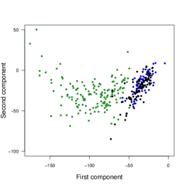
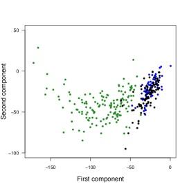
Figure 1: Left: Map of the projection of the data on the original principal components. Right: Map of the projection of the data on the blinded based principal components. Blue: Disk Hernia patients. Black: Normal patients. Green: Spondylolisthesis patients.

The plot on the first two principal components for the example data looks very similar to the plot on the principal components calculated using our procedure (Figure 1). It also shows that the patients with spondylolisthesis are separated from the rest of the patients, but the normal patients and the patients with disc hernias are mixed up together.

Next, we calculate the two principal components using the traditional method and our procedure for the subset of normal and disc hernia patients, using now two variables. The first two principal components explain 75% of the variance then we decide to keep them. We discard to select one variable because in that case the largest angle is close to $78$ degrees. For two variables the largest angle is close to $21$ degrees and for three variables the angle does not decrease very much ($19$ degrees), so we decide to keep two variables.

We consider both, the Euclidean and the Mahalanobis distance, and in both cases the variables selected are “lumbar lordosis angle” and “pelvic radius”. The value of the objective function (2.9) with the Euclidean distance is $0.125$, while with the Mahalanobis distance is $0.141$. Figure 2 shows that the plots for the principal components produced by these procedures look very similar.

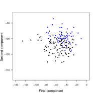
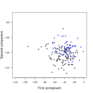
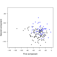
Figure 2: Left: Map of the projection of the data on the original principal components. Middle: Map of the projection of the data on the blinded based principal components using Euclidean distance. Right: Map of the projection of the data on the blinded based principal components using Mahalanobis distance. Blue: Disk Hernia patients. Black: Normal patients.

5 Conclusions

In this paper we introduce a new variable selection procedure for PCA that aim to gain interpretation in principal components.

On one hand we consider a local approach where we deals with finding a subset of variables that best explains each principal component, and on the other hand we analyzed a global approach when the objective is to find a unique subset to explain the first $q$ principal components at once.

We explained how through the conditional expectation we can choose the variables.

Under wide regular conditions in the conditional expectation estimates and on the covariance matrix, strong consistency results are studied and numerical aspects have also been analysed.

The performance of the procedure has been compared with several well-known variable selection techniques using real and simulated data sets, showing the strengths of the method.

Appendix: Proof of Theorem 2.1.

First we are going to proof the following Proposition:

Proposition.

For $k\in\{1,...,p\}$, if

$$\hat{h}^{k}_{n}(I)\rightarrow h^{k}(I)\text{ a.s. for all }I\in\mathcal{I}_{d},$$ (5.1)

then it converges uniformly, and

$$arg\min_{I\in\mathcal{I}_{d}}\hat{h}^{k}_{n}(I)\rightarrow arg\min_{I\in\mathcal{I}_{d}}h^{k}(I)\text{ a.s. }$$

Proof.

Since $\mathcal{I}_{d}$ is a discrete and finite space , the convergence of (5.1) is uniform.

For the sake of simplicity, let $k=1$ (the proof is analogue for $k\in\{2,...,p\}$).

For all $\delta>0$ there exists $n_{0}(\omega)$ such that for every $n\geq n_{0}(\omega)$, with probability one

$$\left|\hat{h}^{1}_{n}(I)-h^{1}(I)\right|<\delta\text{ for all }I\in\mathcal{I}_{d},$$

then,

$$h^{1}(I)-\delta<\hat{h}^{1}_{n}(I)<h^{1}(I)+\delta\text{ for all }I\in\mathcal{I}_{d}$$ (5.2)

and

$$\hat{h}^{1}_{n}(I)-\delta<h^{1}(I)<\hat{h}^{1}_{n}(I)+\delta\text{ for all }I\in\mathcal{I}_{d}.$$ (5.3)

From (2.2), we know that exists $\delta_{0}>0$ such that

$$h^{1}(I_{1})<h^{1}(I)-\delta_{0}\text{ for all }I\notin\mathcal{I}_{1,0},\text{ for all }I_{1}\in\mathcal{I}_{1,0}.$$

By choosing in (5.2) $\delta=\frac{\delta_{0}}{2}$ we obtain

$$\hat{h}^{1}_{n}(I_{1})<h^{1}(I_{1})+\frac{\delta_{0}}{2}<h^{1}(I)-\delta_{0}+\frac{\delta_{0}}{2}=h^{1}(I)-\frac{\delta_{0}}{2}<\hat{h}^{1}_{n}(I)$$

for all $I\notin\mathcal{I}_{1,0}$, for all $I_{1}\in\mathcal{I}_{1,0}$, if $n\geq n_{0}(\omega)$ with probability one.

That means, that there exists $n_{0}(\omega)$ such that, if $n\geq n_{0}(\omega)$, with probability one, if we choose $I_{1}\in\mathcal{I}_{1,0}$, then $I_{1}$ minimizes $\hat{h}^{1}_{n}(I)$.

Moreover, from (2.8), we have that for each $n$ fix, exists $\delta_{1}>0$, such that

$$\hat{h}^{1}_{n}(I^{1})<\hat{h}^{1}_{n}(I)-\delta_{1}\text{ for all }I\notin\hat{I}_{1n},\text{ for all }I^{1}\in\hat{I}_{1n}.$$

Let $\delta=\frac{\delta_{1}}{2}$ in (5.3) and $n\geq n_{1}(\omega)$,

$$h^{1}(I^{1})<\hat{h}^{1}_{n}(I^{1})+\frac{\delta_{1}}{2}<\hat{h}^{1}_{n}(I)-\delta_{1}+\frac{\delta_{1}}{2}=\hat{h}^{1}_{n}(I)-\frac{\delta_{1}}{2}<h^{1}(I)$$

for all $I\notin\hat{I}_{1n}$, and for all $I^{1}\in\hat{I}_{1n}$ with probability one.

That means, that exists $n_{1}(\omega)$ such that, if $n\geq n_{1}(\omega)$ for all $I^{1}\in\hat{I}_{1n}$, $I^{1}$ minimizes $h^{1}(I)$ with probability one.

In conclusion, if $n>max\{n_{0},n_{1}\}$, for all $I_{1}\in\mathcal{I}_{1,0}$, $I_{1}$ minimizes $\hat{h}^{1}_{n}(I)$ and for all $I^{1}\in\hat{I}_{1n}$, $I^{1}$ minimizes $h^{1}(I)$ with probability one.

As the proof is analogue for $k\in\{2,...,p\}$,

$$\mathcal{I}_{k,0}=argmin_{I\in\mathcal{I}_{d}}h^{k}(I),$$

and

$$\hat{I}_{kn}=argmin_{I\in\mathcal{I}_{d}}\hat{h}^{k}_{n}(I)$$

this implies,

$$arg\min_{I\in\mathcal{I}_{d}}\hat{h}^{k}_{n}(I)\rightarrow arg\min_{I\in\mathcal{I}_{d}}h^{k}(I)\text{ a.s. for }k\in\{1,...,p\}.$$

∎

Proof.

(of Theorem)

To prove the Theorem 2.1 then it is enough to see that for each $I$ the empirical objective function (2.8) converges a.s. to the theoretical objective function (2.3). To prove it, let us see that

$$\left\|\hat{\alpha}_{n}^{k}(\mathbb{P}_{n})-\hat{\alpha}_{n}^{k}(\mathbb{P}_{n,\textbf{Y}^{I}})\right\|\rightarrow\left\|\alpha^{k}(\mathbb{P})-\alpha^{k}(\mathbb{P}_{\textbf{Y}^{I}})\right\|\ \text{ a.s. for all }k.$$

Dauxois et al. (1982) proved that under H1, if

$$\left\|\hat{\Sigma}_{n}-\Sigma\right\|_{\infty}=\underset{\left\|u\right\|=1}{max}\left\|\left(\hat{\Sigma}_{n}-\Sigma\right)\left(u\right)\right\|\rightarrow 0\ a.s.,$$

then

$$\left\|\hat{\alpha}^{k}_{n}(\mathbb{P}_{n})-\alpha^{k}(\mathbb{P})\right\|\rightarrow 0\ \text{ a.s. for all }1\leq k\leq p,$$

where $\hat{\alpha}^{k}_{n}(\mathbb{P}_{n})$ (respec. $\alpha^{k}(\mathbb{P})$) are the eigenvectors of $\hat{\Sigma}_{n}$, that denotes the empirical covariance matrix associated with $\mathbb{P}_{n}$ (respec. $\Sigma$ denotes the covariance matrix associated with $\mathbb{P}$).

So, if we prove that

$$\underset{\left\|u\right\|=1}{max}\left\|\left(\hat{\Sigma}_{n}(I)-\Sigma(I)\right)\left(u\right)\right\|\rightarrow 0\ a.s.$$

then

$$\|\hat{\alpha}^{k}_{n}(\mathbb{P}_{n,\mathbf{Y}^{I}})-\alpha^{k}(\mathbb{P}_{\mathbf{Y}^{I}})\|\to 0\ \ a.s.\ \ \forall 1\leq k\leq p,$$

where $\hat{\alpha}^{k}_{n}(\mathbb{P}_{n,\mathbf{Y}^{I}})$ (respec. $\alpha^{k}(\mathbb{P}_{\mathbf{Y}^{I}})$) are the eigenvectors of $\hat{\Sigma}_{n}(I)$, that denotes the empirical covariance matrix associated with $\mathbb{P}_{n,\mathbf{Y}^{I}}$ (respec. $\Sigma(I)$ denotes the covariance matrix associated with $\mathbb{P}_{\mathbf{Y}^{I}}$).

Note, that $I=\{1,\ldots,p\}$ is the classic case. We will show that this also holds for any $I\subseteq\{1,\ldots,p\}$, that is

$$\underset{\left\|u\right\|=1}{max}\left\|\left(\hat{\Sigma}_{n}(I)-\Sigma(I)\right)\left(u\right)\right\|\rightarrow 0\ a.s.$$

To simplify the notation, we can assume (without losing generality) that $I=\{1,\ldots,d\}$, then

$$\mathbf{Y}_{j}=\left(X_{j}[1],\ldots,X_{j}[d],g^{1}_{n}(\mathbf{X}_{j}[I]),\ldots,g^{p-d}_{n}(\mathbf{X}_{j}[I])\right)^{t},$$

where $g^{i}_{n}(z)$ is a uniformly consistent nonparametric estimate of $g^{i}(z)$. Specifically, $g^{i}_{n}$ will fulfil the following assumption,

$$g_{n}^{l}(\mathbf{X}_{j}[I])\rightarrow g^{l}(\mathbf{X}_{j}[I])\ a.s.\text{ for any $l$, for all $j$, uniformly}.$$

We define a non observable auxiliary vector,

$$\mathbf{Z}_{j}=\left(X_{j}[1],\ldots,X_{j}[d],g^{1}(\mathbf{X}_{j}[I]),\ldots,g^{p-d}(\mathbf{X}_{j}[I])\right)^{t},$$

where $g^{i}(z)=E(X[d+i]|\mathbf{X}[I]=z)$.

The proof will be complete if we show that

$$\underset{\left\|u\right\|=1}{max}\left\|\left(\Sigma_{\mathbf{Z}}-\Sigma(I)\right)\left(u\right)\right\|\rightarrow 0\ a.s.,$$ (5.4)

and that

$$\underset{\left\|u\right\|=1}{max}\left\|\left(\Sigma_{\mathbf{Y}}-\Sigma_{\mathbf{Z}}\right)\left(u\right)\right\|\rightarrow 0\ a.s.,$$ (5.5)

where $\Sigma_{\mathbf{Y}}=\hat{\Sigma}_{n}(I)$.

Considering,

$$\overline{X[i]}=\frac{1}{n}\sum_{j=1}^{n}X_{j}[i],\quad\overline{g_{n}^{l}(\mathbf{X}[I])}=\frac{1}{n}\sum_{j=1}^{n}g_{n}^{l}(\mathbf{X}_{j}[I]),\quad\overline{g^{l}(\mathbf{X}[I])}=\frac{1}{n}\sum_{j=1}^{n}g^{l}(\mathbf{X}_{j}[I])$$

the three matrices are

$$(\Sigma(I))_{ii^{\prime}}=\left\{\begin{array}[]{cccc}cov(X[i],X[i^{\prime}])\text{ if}\ 1\leq i,i^{\prime}\leq d,\\ cov(X[i],\mathbb{E}(X[i^{\prime}]|\mathbf{X}[I]))\text{ if }1\leq i\leq d<i^{\prime}\leq p,\\ cov(\mathbb{E}(X[i]|\mathbf{X}[I]),X[i^{\prime}])\text{ if }1\leq i^{\prime}\leq d<i\leq p,\\ cov(\mathbb{E}(X[i]|\mathbf{X}[I]),\mathbb{E}(X[i^{\prime}]|\mathbf{X}[I]))\text{ if }d+1\leq i,i^{\prime}\leq p,\end{array}\right.$$

$$(\Sigma_{\mathbf{Y}})_{ii^{\prime}}=\left\{\begin{array}[]{cccc}\frac{1}{n}\sum_{j=1}^{n}(X_{j}[i]-\overline{X[i]})(X_{j}[i^{\prime}]-\overline{X[i^{\prime}]})\text{ if }1\leq i,i^{\prime}\leq d,\\ \frac{1}{n}\sum_{j=1}^{n}(X_{j}[i]-\overline{X[i]})(g_{n}^{i^{\prime}-d}(\mathbf{X}_{j}[I])-\overline{g_{n}^{i^{\prime}-d}(\mathbf{X}[I])})\text{ if }1\leq i\leq d<i^{\prime}\leq p,\\ \frac{1}{n}\sum_{j=1}^{n}(g_{n}^{i-d}(\mathbf{X}_{j}[I])-\overline{g_{n}^{i-d}(\mathbf{X}[I])})(X_{j}[i^{\prime}]-\overline{X[i^{\prime}]})\text{ if }1\leq i^{\prime}\leq d<i\leq p,\\ \frac{1}{n}\sum_{j=1}^{n}(g_{n}^{i-d}(\mathbf{X}_{j}[I])-\overline{g_{n}^{i-d}(\mathbf{X}[I])})(g_{n}^{i^{\prime}-d}(\mathbf{X}_{j}[I])-\overline{g_{n}^{i^{\prime}-d}(\mathbf{X}[I])})\text{ if }d+1\leq i,i^{\prime}\leq p,\end{array}\right.$$

$$(\Sigma_{\mathbf{Z}})_{ii^{\prime}}=\left\{\begin{array}[]{cccc}\frac{1}{n}\sum_{j=1}^{n}(X_{j}[i]-\overline{X[i]})(X_{j}[i^{\prime}]-\overline{X[i^{\prime}]})\text{ if }1\leq i,i^{\prime}\leq d,\\ \frac{1}{n}\sum_{j=1}^{n}(X_{j}[i]-\overline{X[i]})(g^{i^{\prime}-d}(\mathbf{X}_{j}[I])-\overline{g^{i^{\prime}-d}(\mathbf{X}[I])})\text{ if }1\leq i\leq d<i^{\prime}\leq p,\\ \frac{1}{n}\sum_{j=1}^{n}(g^{i-d}(\mathbf{X}_{j}[I])-\overline{g^{i-d}(\mathbf{X}[I])})(X_{j}[i^{\prime}]-\overline{X[i^{\prime}]})\text{ if }1\leq i^{\prime}\leq d<i\leq p,\\ \frac{1}{n}\sum_{j=1}^{n}(g^{i-d}(\mathbf{X}_{j}[I])-\overline{g^{i-d}(\mathbf{X}[I])})(g^{i^{\prime}-d}(\mathbf{X}_{j}[I])-\overline{g^{i^{\prime}-d}(\mathbf{X}[I])})\text{ if }d+1\leq i,i^{\prime}\leq p.\end{array}\right.$$

We will now prove the convergence in (5.4) and (5.5).

First, we show that

$$\underset{\left\|u\right\|=1}{max}\left\|\left(\Sigma_{\mathbf{Z}}-\Sigma(I)\right)\left(u\right)\right\|\rightarrow 0\ a.s.$$

It is sufficient to prove that each of the coordinates of the matrix $\Sigma_{\mathbf{Z}}-\Sigma(I)$ converge to zero.

Set $1\leq i,i^{\prime}\leq p$, then $(\Sigma_{\mathbf{Z}})_{ii^{\prime}}\rightarrow(\Sigma(I))_{ii^{\prime}}\ a.s.$ and then $(\Sigma_{\mathbf{Z}}-\Sigma(I))_{ii^{\prime}}\rightarrow 0\ a.s.$ $\forall i,i^{\prime}=1,...,p$.

Because we are using a finite dimensional space, and each of the coordinates converge to zero, it holds that

$$\underset{\left\|u\right\|=1}{max}\left\|\left(\Sigma_{\mathbf{Z}}-\Sigma(I)\right)\left(u\right)\right\|\rightarrow 0\ a.s.$$

Now, we show that

$$\underset{\left\|u\right\|=1}{max}\left\|\left(\Sigma_{\mathbf{Y}}-\Sigma_{\mathbf{Z}}\right)\left(u\right)\right\|\rightarrow 0\ a.s.$$

As before, we are going to prove that each of the coordinates of the matrix $\Sigma_{\mathbf{Y}}-\Sigma_{\mathbf{Z}}$ converge to zero.

For better understanding, we define

$$\mathcal{G}(l,j,n)=g_{n}^{l}(\mathbf{X}_{j}[I])-\overline{g_{n}^{l}(\mathbf{X}[I])}-g^{l}(\mathbf{X}_{j}[I])+\overline{g^{l}(\mathbf{X}[I])}.$$

$\bullet$ If $1\leq i,i^{\prime}\leq d$, $(\Sigma_{\mathbf{Y}})_{ii^{\prime}}=(\Sigma_{\mathbf{Z}})_{ii^{\prime}}$ then $(\Sigma_{\mathbf{Y}}-\Sigma_{\mathbf{Z}})_{ii^{\prime}}=0$.

$\bullet$ If $1\leq i\leq d,d+1\leq i^{\prime}\leq p$,

$$(\Sigma_{\mathbf{Y}}-\Sigma_{\mathbf{Z}})_{ii^{\prime}} = \frac{1}{n}\sum_{j=1}^{n}(X_{j}[i]-\overline{X[i]})(g_{n}^{i^{\prime}-d}(\mathbf{X}_{j}[I])-\overline{g_{n}^{i^{\prime}-d}(\mathbf{X}[I])}-g^{i^{\prime}-d}(\mathbf{X}_{j}[I])+\overline{g^{i^{\prime}-d}(\mathbf{X}[I])})$$

$$= \frac{1}{n}\sum_{j=1}^{n}(X_{j}[i]-\overline{X[i]})\mathcal{G}(i^{\prime}-d,j,n).$$

From the Cauchy-Schwarz inequality, we have that

$$\left|\frac{1}{n}\sum_{j=1}^{n}(X_{j}[i]-\overline{X[i]})\mathcal{G}(i^{\prime}-d,j,n)\right|\leq\left(\frac{1}{n}\sum_{j=1}^{n}(X_{j}[i]-\overline{X[i]})^{2}\right)^{\frac{1}{2}}\left(\frac{1}{n}\sum_{j=1}^{n}(\mathcal{G}(i^{\prime}-d,j,n))^{2}\right)^{\frac{1}{2}}$$

On the other hand,

$$\frac{1}{n}\sum_{j=1}^{n}(X_{j}[i]-\overline{X[i]})^{2}\rightarrow Var(X[i])\ a.s.$$ (5.9)

In addition, since

$$g_{n}^{l}(\mathbf{X}_{j}[I])\rightarrow g^{l}(\mathbf{X}_{j}[I])\ a.s.\text{ uniformly, for any $l$, for all $j$},$$

then for any l,

$$\overline{g_{n}^{l}(\mathbf{X}[I])}-\overline{g^{l}(\mathbf{X}[I])}=\frac{1}{n}\sum_{j=1}^{n}g_{n}^{l}(\mathbf{X}_{j}[I])-g^{l}(\mathbf{X}_{j}[I])\leq\max_{1\leq j\leq n}\{g_{n}^{l}(\mathbf{X}_{j}[I])-g^{l}(\mathbf{X}_{j}[I])\}\rightarrow 0\ a.s.$$

and therefore,

$$\mathcal{G}(l,j,n)\rightarrow 0\ a.s.\text{ for any $l$, for all $j$}.$$

This implies

$$\frac{1}{n}\sum_{j=1}^{n}(\mathcal{G}(l,j,n))^{2}\rightarrow 0\ a.s.\text{ for any $l$}.$$ (5.10)

Thus, by (5.9) and (5.10) we have

$$\left|\frac{1}{n}\sum_{j=1}^{n}(X_{j}[i]-\overline{X[i]})\mathcal{G}(i^{\prime}-d,j,n)\right|\rightarrow 0\ a.s.$$ (5.11)

which is what we required for our proof.

$\bullet$ If $d+1\leq i\leq p,1\leq i^{\prime}\leq d$, from the simetry of the matrices and (5.11), we have that $(\Sigma_{\mathbf{Y}}-\Sigma_{\mathbf{Z}})_{ii^{\prime}}\rightarrow 0\ a.s.$

$\bullet$ If $d+1\leq i\leq p,d+1\leq i^{\prime}\leq p$,

$$(\Sigma_{\mathbf{Y}}-\Sigma_{\mathbf{Z}})_{ii^{\prime}} = \frac{1}{n}\sum_{j=1}^{n}\left[(g_{n}^{i-d}(\mathbf{X}_{j}[I])-\overline{g_{n}^{i-d}(\mathbf{X}[I])})(g_{n}^{i^{\prime}-d}(\mathbf{X}_{j}[I])-\overline{g_{n}^{i^{\prime}-d}(\mathbf{X}[I])})\right]-$$

$$\left[(g^{i-d}(\mathbf{X}_{j}[I])-\overline{g^{i-d}(\mathbf{X}[I])})(g^{i^{\prime}-d}(\mathbf{X}_{j}[I])-\overline{g^{i^{\prime}-d}(\mathbf{X}[I])})\right].$$

If we add and subtract $(g^{i-d}(\mathbf{X}_{j}[I])-\overline{g^{i-d}(\mathbf{X}[I])})(g_{n}^{i^{\prime}-d}(\mathbf{X}_{j}[I])-\overline{g_{n}^{i^{\prime}-d}(\mathbf{X}[I])})$, and rearrange, we get that $(\Sigma_{\mathbf{Y}}-\Sigma_{\mathbf{Z}})_{ii^{\prime}}$ is the sum of

$$\frac{1}{n}\sum_{j=1}^{n}(g_{n}^{i^{\prime}-d}(\mathbf{X}_{j}[I])-\overline{g_{n}^{i^{\prime}-d}(\mathbf{X}[I])})\mathcal{G}(i-d,j,n)$$ (5.12)

and

$$\frac{1}{n}\sum_{j=1}^{n}(g^{i-d}(\mathbf{X}_{j}[I])-\overline{g^{i-d}(\mathbf{X}[I])})\mathcal{G}(i^{\prime}-d,j,n)$$

were (5.12) can be rewrited as

$$\frac{1}{n}\sum_{j=1}^{n}[\mathcal{G}(i^{\prime}-d,j,n)+(g^{i^{\prime}-d}(\mathbf{X}_{j}[I])-\overline{g^{i^{\prime}-d}(\mathbf{X}[I])})]\mathcal{G}(i-d,j,n)$$

or

$$\frac{1}{n}\sum_{j=1}^{n}\mathcal{G}(i^{\prime}-d,j,n)\mathcal{G}(i-d,j,n)+\frac{1}{n}\sum_{j=1}^{n}(g^{i^{\prime}-d}(\mathbf{X}_{j}[I])-\overline{g^{i^{\prime}-d}(\mathbf{X}[I])})\mathcal{G}(i-d,j,n).$$

Then we have that

$$(\Sigma_{\mathbf{Y}}-\Sigma_{\mathbf{Z}})_{ii^{\prime}} = \frac{1}{n}\sum_{j=1}^{n}\mathcal{G}(i^{\prime}-d,j,n)\mathcal{G}(i-d,j,n)$$

$$+ \frac{1}{n}\sum_{j=1}^{n}(g^{i^{\prime}-d}(\mathbf{X}_{j}[I])-\overline{g^{i^{\prime}-d}(\mathbf{X}[I])})\mathcal{G}(i-d,j,n)$$

$$+ \frac{1}{n}\sum_{j=1}^{n}(g^{i-d}(\mathbf{X}_{j}[I])-\overline{g^{i-d}(\mathbf{X}[I])})\mathcal{G}(i^{\prime}-d,j,n).$$

From triangular and Cauchy-Schwarz inequality,

$$\left|(\Sigma_{\mathbf{Y}}-\Sigma_{\mathbf{Z}})_{ii^{\prime}}\right| \leq \left(\frac{1}{n}\sum_{j=1}^{n}(\mathcal{G}(i^{\prime}-d,j,n))^{2}\right)^{1/2}\left(\frac{1}{n}\sum_{j=1}^{n}(\mathcal{G}(i-d,j,n))^{2}\right)^{1/2}$$

$$+ \left(\frac{1}{n}\sum_{j=1}^{n}(g^{i^{\prime}-d}(\mathbf{X}_{j}[I])-\overline{g^{i^{\prime}-d}(\mathbf{X}[I])})^{2}\right)^{1/2}\left(\frac{1}{n}\sum_{j=1}^{n}(\mathcal{G}(i-d,j,n))^{2}\right)^{1/2}$$

$$+ \left(\frac{1}{n}\sum_{j=1}^{n}(g^{i-d}(\mathbf{X}_{j}[I])-\overline{g^{i-d}(\mathbf{X}[I])})^{2}\right)^{1/2}\left(\frac{1}{n}\sum_{j=1}^{n}(\mathcal{G}(i^{\prime}-d,j,n))^{2}\right)^{1/2}$$

On the other hand, we have that

$$\frac{1}{n}\sum_{j=1}^{n}(g^{l}(\mathbf{X}_{j}[I])-\overline{g^{l}(\mathbf{X}[I])})^{2}\rightarrow Var(g^{l}(\mathbf{X}[I]))\ a.s.\text{ for any $l$}.$$

If $Var(g^{l}(\mathbf{X}[I]))<\infty$ for any $l$ and $I$, (5.10) entails $\left|(\Sigma_{\mathbf{Y}}-\Sigma_{\mathbf{Z}})_{ii^{\prime}}\right|\to 0$.

As $Var(X[l])<\infty$, then for any $l$ and any $I$,

$$Var(X[l])=E(Var(X[l]|\mathbf{X}[I]))+Var(E(X[l]|\mathbf{X}[I]))=E(Var(X[l]|\mathbf{X}[I]))+Var(g^{l}(\mathbf{X}[I]))$$

We now that $E(Var(X[l]|\mathbf{X}[I]))>0$, so we conclude that $Var(g^{l}(\mathbf{X}[I]))<\infty$

We have proved that all the coordinates of the matrix $\Sigma_{\mathbf{Y}}-\Sigma_{\mathbf{Z}}$ converge to zero, so

$$\underset{\left\|u\right\|=1}{sup}\left\|\left(\Sigma_{\mathbf{Y}}-\Sigma_{\mathbf{Z}}\right)\left(u\right)\right\|\rightarrow 0\ a.s.$$

Now we are ready to complete the proof of Theorem 2.1. From (5.4) and (5.5) we are able to use the result from Dauxois et al. (1982) to derive that,

$$\hat{h}^{k}_{n}(I)=\|\hat{\alpha}^{k}_{n}(\mathbb{P}_{n})-\hat{\alpha}^{k}_{n}(\mathbb{P}_{n,\mathbf{Y}^{I}})\|^{2}\to\|\alpha^{k}(\mathbb{P})-\alpha^{k}(\mathbb{P}_{\mathbf{Y}^{I}})\|^{2}=h^{k}(I)\ \ a.s.$$ (5.13)

Indeed, we have that

$$\|\hat{\alpha}^{k}_{n}(\mathbb{P}_{n})-\hat{\alpha}^{k}_{n}(\mathbb{P}_{n,\mathbf{Y}^{I}})\|-\|\alpha^{k}(\mathbb{P})-\alpha^{k}(\mathbb{P}_{\mathbf{Y}^{I}})\|\leq$$

$$\|\hat{\alpha}^{k}_{n}(\mathbb{P}_{n})-\alpha^{k}(\mathbb{P})\|+\|\alpha^{k}(\mathbb{P})-\alpha^{k}(\mathbb{P}_{\mathbf{Y}^{I}})\|+$$

$$\|\alpha^{k}(\mathbb{P}_{\mathbf{Y}^{I}})-\hat{\alpha}^{k}_{n}(\mathbb{P}_{n,\mathbf{Y}^{I}})\|-\|\alpha^{k}(\mathbb{P})-\alpha^{k}(\mathbb{P}_{\mathbf{Y}^{I}})\|=$$

$$\|\hat{\alpha}^{k}_{n}(\mathbb{P}_{n})-\alpha^{k}(\mathbb{P})\|+\|\alpha^{k}(\mathbb{P}_{\mathbf{Y}^{I}})-\hat{\alpha}^{k}_{n}(\mathbb{P}_{n,\mathbf{Y}^{I}})\|\to 0\ a.s.$$

and

$$\|\alpha^{k}(\mathbb{P})-\alpha^{k}(\mathbb{P}_{\mathbf{Y}^{I}})\|-\|\hat{\alpha}^{k}_{n}(\mathbb{P}_{n})-\hat{\alpha}^{k}_{n}(\mathbb{P}_{n,\mathbf{Y}^{I}})\|\leq$$

$$\|\alpha^{k}(\mathbb{P})-\hat{\alpha}^{k}_{n}(\mathbb{P}_{n})\|+\|\hat{\alpha}^{k}_{n}(\mathbb{P}_{n})-\hat{\alpha}^{k}_{n}(\mathbb{P}_{n,\mathbf{Y}^{I}})\|+$$

$$\|\hat{\alpha}^{k}_{n}(\mathbb{P}_{n,\mathbf{Y}^{I}})-\alpha^{k}(\mathbb{P}_{\mathbf{Y}^{I}})\|-\|\hat{\alpha}^{k}_{n}(\mathbb{P}_{n})-\hat{\alpha}^{k}_{n}(\mathbb{P}_{n,\mathbf{Y}^{I}})\|=$$

$$\|\alpha^{k}(\mathbb{P})-\hat{\alpha}^{k}_{n}(\mathbb{P}_{n})\|+\|\hat{\alpha}^{k}_{n}(\mathbb{P}_{n,\mathbf{Y}^{I}})-\alpha^{k}(\mathbb{P}_{\mathbf{Y}^{I}})\|\to 0\ a.s.$$

which entails (5.13).

Finally, (5.13) and the Proposition implies

$$arg\min_{I\in\mathcal{I}_{d}}\hat{h}^{k}_{n}(I)\rightarrow arg\min_{I\in\mathcal{I}_{d}}h^{k}(I)\text{ a.s. }$$

which concludes the proof.

∎

References

- Biau et al. (2013) Biau, G., Fischer, A., Guedj, B. and Malley, J.D. (2013), “COBRA: A collective regression strategy”, arxiv.org/pdf/1303.2236.
- Dauxois et al. (1982) Dauxois, J., Pousse, A. and Romain, Y., (1982),“Asymptotic theory for the principal component analysis of a vector random function: some applications to statistical inference”, Journal of Multivariate Analysis 12, 136–154.
- Fraiman et al. (2008) Fraiman, R., Justel, A. and Svarc, M., (2008), “Selection of variables for cluster analysis and classification rules”, Journal of the American Statistical Association. 103(483), 1294–1303.
- Frank & Asuncion (2010) Frank, A. and Asuncion, A., (2010), UCI Machine Learning Repository [http://archive.ics.uci.edu/ml], Irvine, CA: University of California, School of Information and Computer Science.
- Hansen (2008) Hansen, B.E. (2008), “Uniform convergence rates for kernel estimation with dependent data”, Econometric Theory. 24, 726–748.
- He & Shi (1996) He, X. and Shi, P., (1996), “Bivariate Tensor-Product B-Splines in Partly Linear Models”, Journal of Multivariate Analysis. 58, 162–181.
- Jolliffe (1995) Jolliffe, I., (1995), “ Rotation of principal components: choise of normalization constraints”, Journal of Applied Statistics.22, 29–35.
- Jolliffe (2002) Jolliffe, I. (2002), “Principal Components Analysis. Second Edition”, Ed. Springer.
- Jolliffe et al. (2003) Jolliffe, I., Trendafilov, N. and Uddin, M. (2003), “ A modified principal component technique based on the LASSO”, Journal of Computational and Graphical Statistics. 12, 531–547.
- Li & Gong (1987) Li, R. and Gong, G. (1987), “K-nn Nonparametric Estimation Of Regression Functions In the Presence of Irrelevant Variables”, Econometrics Journal, 00, 1-12.
- Luss & d’Aspremont (2010) Luss, R. and d’Aspremont, A., (2010), “Clustering and feature selection using sparse principal component analysis”, Optimization and Engineering. 11(1), 145–157.
- Maronna et al. (2006) Maronna, R. A., Martin, R. D. and Yohai, V. J., (2006), “Robust Statistics: Theory and Methods”, Wiley, London.
- McCabe (1984) McCabe, G. P. (1984), “Principal Variables”, Technometrics. 26, 137–144.
- Tibshirani (1996) Tibshirani, R., (1996), “Regression shrinkage and selection via the LASSO”, Journal of the Royal statistical society. Series B 58(1), 267–288.
- Vines (2000) Vines,S., (2000), “Simple principal components”, Applied Statistics. 49, 441–451.
- Witten & Tibshirani (2008) Witten, D.M. and Tibshirani, R., (2008), “Testing significance of features by lassoed principal components”, Annals of Applied Statistics. 2(3), 986–1012.
- Zou & Hastie (2005) Zou, H. and Hastie, T., (2005), “‘Regularizations and variable selection via the elastic net”, Journal of the Royal Statistical Society. Series B, 67, 301–320.
- Zou et al. (2006) Zou, H., Hastie, T. and Tibshirani, R. (2006), “Sparse principal component analysis”, Journal of Computational and Graphical Statistics, 15, 265–286.