Backward stochastic differential equation approach to modeling of gene expression

Abstract

In this article, we introduce a novel backward method to model stochastic gene expression and protein level dynamics. The protein amount is regarded as a diffusion process and is described by a backward stochastic differential equation (BSDE). Unlike many other SDE techniques proposed in the literature, the BSDE method is backward in time; that is, instead of initial conditions it requires the specification of endpoint (“final”) conditions, in addition to the model parametrization. To validate our approach we employ Gillespie’s stochastic simulation algorithm (SSA) to generate (forward) benchmark data, according to predefined gene network models. Numerical simulations show that the BSDE method is able to correctly infer the protein level distributions that preceded a known final condition, obtained originally from the forward SSA. This makes the BSDE method a powerful systems biology tool for time reversed simulations, allowing, for example, the assessment of the biological conditions (e.g. protein concentrations) that preceded an experimentally measured event of interest (e.g. mitosis, apoptosis, etc.).

I Introduction

Gene regulatory networks involving small numbers of molecules can be intrinsically noisy and subject to large protein concentration fluctuations Thattai and van Oudenaarden (2001); Ozbudak et al. (2002). This fact substantially limits the ability to infer the causal relations within gene regulatory networks and the ability to understand the mechanisms involved in healthy and pathological conditions. A large interest has been raised in developing tools for gene regulatory network inference Karlebach and Shamir (2008); Hecker et al. (2009) acknowledging the noisy/stochastic properties of experimental data Mettetal et al. (2006); Wilkinson (2011); Lillacci and Khammash (2013), in parallel with studies addressing the prospective, forward, simulation of stochastic equations describing biochemical reactions Gillespie (1977). There is, however, another context which, despite its relevance as a tool to better understand intracellular dynamics, has received little attention from a mathematical modeling perspective. That is the situation where the basic gene regulatory network is known, together with a present distribution of molecules/proteins, and one wants to infer the previous molecules distributions that gave rise to the observed data. This is the case, for example, of a sample of necrotic cells where the concentration distributions for the relevant molecules can be calculated, and one would like to infer the previous concentrations that gave rise to the necrotic condition. In this context, the problem can be addressed with backward stochastic differential equations.

BSDEs were introduced by Bismut in 1973 Bismut (1973), and over the last twenty years have been extensively studied by many mathematicians (e.g. Pardoux and Pend (1990), Ma et al. (1994)).

In what follows, we present a method to model gene expression based on backward stochastic differential equations. We consider a gene regulatory network, where the stochastic variables are the amounts of proteins that are expressed from the genes of the network. To illustrate our method, we apply it to four simple gene networks: a positive self-regulating gene, which is the simplest network, networks composed by two and five interacting genes, and a bistable two-gene network. To generate data to test and validate our approach we use Gillespie’s stochastic simulation algorithm, referred to below as SSA (Gillespie (1977)), for simulation of biochemical reactions. From the trajectories of multiple simulations, the SSA provides the distribution of protein amounts at a fixed final time, as well as at some fixed moments of time prior to the final. For realization of the SSA we used the COPASI software cop . The network models used in the BSDE and the SSA simulations were taken the same. The BSDE method, which requires the final distribution as the input data, was applied to perform a simulation backwards in time. Importantly, at the end of the backward simulation we arrive at some deterministic value for the number of proteins which is very close to the SSA initial condition. Since in many applications the initial protein amounts are not known, and are, in fact, the goal of the study, we believe that our approach can be a useful tool in systems biology.

II The BSDE method

In what follows, we describe the BSDE method to model gene expression. Specifically, we model the dynamics of protein amounts expressed by the genes of a gene regulatory network. In our simulation, the protein synthesis and degradation occurs on the time interval $[t_{0},T]$. The input data for the BSDE method is the protein number distribution at time $T$. The amount of proteins is modeled by a continuous ${\mathbb{R}}^{n}$-valued diffusion process $\eta_{t}=(\eta_{1}(t),\eta_{2}(t),\ldots,\eta_{n}(t))$, where $n$ is the amount of species, or types of proteins expressed by the genes of the network, and $\eta_{i}(t)$ is the amount of the $i$-th type of protein at time $t$.

In our model, the transcription and translation are treated effectively as a single process. In other words, we assume that different mRNAs transcribed from the gene are translated at the same rate.

II.1 General description of the method

In the BSDE method, the evolution of $\eta_{t}$ is governed by the following BSDE

$$\eta_{t}=\eta_{T}-\int_{t}^{T}f(\eta_{s})\,ds-\int_{t}^{T}z_{s}\,dW_{s},\;t\in[t_{0},T].$$ (1)

On the right-hand side, $\eta_{T}$ is the vector of final amounts of proteins whose distribution at time $T$ is known, the second term is a drift that represents the regulation of the protein production, and the last term is an unknown noise that makes the solution $\eta_{t}$ stochastic. Furthermore, $W_{s}$ is a real-valued Wiener process (also referred to below as a Brownian motion), and $f$ is an ${\mathbb{R}}^{n}$-valued synthesis/degradation rate of the proteins under regulation whose explicit form is discussed in detail in Section III.1. Rigorously speaking, the last term in (1) is an Itô stochastic integral with respect to the Brownian motion $W_{s}$, where the integrand $z_{s}$ is an unknown stochastic process.

In order to solve BSDE (1) numerically we represent $\eta_{T}$ in the form $h(W_{T})$, where $h(x)$ is a continuous function defined for real values $x$ and taking values in ${\mathbb{R}}^{n}$. This function will be obtained numerically during the realization of our method. The main tool for obtaining a numerical solution to (1) is the following deterministic final value problem with respect to an unknown ${\mathbb{R}}^{n}$-valued function $\theta(t,x)$ defined for $(t,x)\in[t_{0},T]\times{\mathbb{R}}$:

$$\begin{cases}\partial_{t}\theta(t,x)+\frac{1}{2}\theta_{xx}(t,x)-f(\theta(t,x))=0,\\ \theta(T,x)=h(x),\quad x\in{\mathbb{R}}.\end{cases}$$ (2)

In the above PDE, the variable $x$ is an abstract variable that is to be substituted by a Wiener process to generate the solution to equation (1), and PDE (2) itself is a tool to obtaining a solution to BSDE (1). Namely, the theory of BSDEs (Ma et al. (1994)) implies that if $\theta(t,x)$ is a solution to problem (2), then the pair of stochastic processes

$$\eta_{t}=\theta(t,W_{t})\quad\text{and}\quad z_{t}=\nabla\theta(t,W_{t})$$ (3)

is the unique solution to (1) under the constraint that $\eta_{t}$ is adapted with respect to $W_{t}$ (see Pardoux and Pend (1990), Ma et al. (1994) for details). The forementioned adaptedness means that for each $t$, $\eta_{t}$ is a function of $W_{t}$. We provide more details about BSDEs in the appendix.

Let us summarize the algorithm of obtaining a numerical solution to BSDE (1). (a) Construct the function $h$ with the property $h(W_{T})=\eta_{T}$; (b) Obtain a numerical solution $\theta(t,x)$ to problem (2); (c) Simulate a sufficient number of Brownian motion trajectories and obtain the solution to (1) in the form $\eta_{t}=\theta(t,W_{t})$.

Let us start with (a). We obtain the distribution of $\eta_{T}$ in the form of a histogram $H$. The ${\mathbb{R}}^{n}$-valued function $h$ is chosen so that the distribution of $h(W_{T})$ produces a histogram approximately equal to $H$. The method of finding the function $h$ and, therefore, obtaining $\eta_{T}$ as $h(W_{T})$, is referred to below as the final data approximation technique.

Let $l_{i}$, $i=1,2,\ldots$, be the bin ends of the given histogram $H$, and $p_{i}$ be the bin probabilities. This means that the probability that $\eta_{T}$ belongs to $[l_{i},l_{i+1}]$ is $p_{i}$. We search $h$ as a piecewise linear continuous increasing function of the form

$$h(x)=\sum_{i=1}^{N}\chi_{[r_{i},r_{i+1})}(x)(k_{i}x+b_{i})$$ (4)

where $\chi_{(r_{i},r_{i+1}]}(x)$ is the characteristic function the interval $[r_{i},r_{i+1})$, i.e. $\chi_{[r_{i},r_{i+1})}(x)=1$ if $x$ belongs to $[r_{i},r_{i+1})$ and it is zero otherwise. We aim to choose $k_{i}$ and $b_{i}$ so that $h(r_{i})=l_{i}$, i.e. $h$ maps $[r_{i},r_{i+1}]$ onto $[l_{i},l_{i+1}]$. Since $\eta_{T}$ is in $[r_{i},r_{i+1}]$ with probability $p_{i}$, the forementioned property of $h$ implies that $W_{T}$ belongs to $[r_{i},r_{i+1}]$ also with probability $p_{i}$. Thus, we produce 20000 realizations of the random variable $W_{T}$. The endpoint $r_{1}$ is choosen as the smallest of the realizations of $W_{T}$. Suppose we constructed the endpoint $r_{i}$. Note that $W_{T}$ is a Gaussian random variable with mean zero and variance $\sqrt{T}$. Let $\Phi_{T}(x)$ be the distribution function of $W_{T}$. Clearly, we can uniquely find the point $r_{i+1}$ so that $\Phi_{T}(r_{i+1})-\Phi_{T}(r_{i})=p_{i}$. Further, we compute $k_{i}=(l_{i+1}-l_{i})/(r_{i+1}-r_{i})$ and choose $b_{i}$ so that $h(x)$ becomes continuous at point $r_{i}$, i.e. $b_{i}=r_{i}(k_{i-1}-k_{i})+b_{i-1}$. Since computing of $b_{1}$ requires $b_{0}$, we set $b_{0}$ to be the mean of $\eta_{T}$.

We remark that continuous function $h$ satisfying $h(W_{T})=\eta_{T}$ may not be unique. However, the goal of the construction of $h$ is to be able to solve BSDE (1) by means of problem (2). From the theory of BSDEs (Pardoux and Pend (1990)) it is known that the $\mathcal{F}_{t}$-adapted solution pair $(\eta_{t},z_{t})$ is, in fact, uniquely determined by the final data $\eta_{T}$.

Now we describe part (b) of the algorithm which is obtaining a numerical solution to (2). By doing the time change $\tilde{\theta}(t,x)=\theta(T-t,x)$ we transform (2) to a Cauchy problem with the initial condition $\tilde{\theta}(0,x)=h(x)$. Note that, by (4), the function $h$ is defined only on a compact interval $[r_{1},r_{N+1}]$ which is the support for all the realizations of $W_{T}$. The values of $h$ outside of this interval do not affect the solution to (1). Therefore, we can extend $h$ to the whole real line ${\mathbb{R}}$ so that the extended function is continuous and its derivative vanishes outside of a compact interval $[a,b]$ containing $[r_{1},r_{N+1}]$. Therefore, in practice, instead of (2) we solve the following initial-boundary value problem:

$$\begin{cases}\partial_{t}\tilde{\theta}(t,x)-\frac{1}{2}\tilde{\theta}_{xx}(t,x)+f(\tilde{\theta}(t,x))=0,\\ \tilde{\theta}(0,x)=h(x),\\ \tilde{\theta}_{x}(t,a)=\tilde{\theta}_{x}(t,b)=0.\end{cases}$$ (5)

Finally, in part (c) we simulate a sufficient number of Brownian motion trajectories $W_{t}$ starting at zero at time $t_{0}$ and obtain the trajectories $\eta_{t}$ as $\theta(t,W_{t})$. In our simulation, we took 20000 trajectories of $W_{t}$. We note that the noise can be computed as the stochastic integral $\int_{t}^{T}\nabla\theta(s,W_{s})dW_{s}$. However, as mentioned earlier, in this work we are only interested in the protein amount process $\eta_{t}$.

II.2 BSDE model for multistability

Here we extend the model described in II.1 to the case when the observed final distribution is bimodal. For simplicity, we describe the method for two-gene networks, although our strategy can be naturally extended for networks composed by more than two genes. The stochastic equation describing the dynamics of proteins synthesis and degradation is still BSDE (1), however we decouple it into two BSDEs and solve each BSDE separately. Namely, we split the set of random parameters $\Omega$ into two disjoint sets $\Omega=\Omega_{A}\cup\Omega_{B}$, and represent the stochastic process $\eta_{t}=(\eta_{1}(t),\eta_{2}(t))$ in the form

$$\eta_{t}=\begin{pmatrix}\eta_{1}(t)\\ \eta_{2}(t)\end{pmatrix}\chi_{\Omega_{A}}+\begin{pmatrix}\eta_{1}(t)\\ \eta_{2}(t)\end{pmatrix}\chi_{\Omega_{B}}=\eta^{A}_{t}+\eta^{B}_{t},$$

where $\chi_{\Omega_{C}}(\omega)$, $C=A,B$, is the characteristic function of the set $\Omega_{C}$ (i.e. $\chi_{\Omega_{C}}(\omega)=1$ if $\omega\in\Omega_{C}$ and $\chi_{\Omega_{C}}(\omega)=0$ otherwise), $\eta^{A}_{t}=\eta_{t}\chi_{\Omega_{A}}$ and $\eta^{B}_{t}=\eta_{t}\chi_{\Omega_{B}}$.

In fact, in SSA numerical experiments involving two-gene networks for some rate functions $f(\eta)$ we observed that protein amount trajectories $\eta_{1}(t)$ and $\eta_{2}(t)$ split into two branches (See Fig. 1).

\begin{overpic}[width=241.84842pt]{fig1-eps-converted-to.pdf} \put(18.0,73.6){\framebox{\minipage{433.62pt}{Protein number trajectories:} \\ {Multistability in a 2-gene network} \endminipage}} \end{overpic}

Figure 1: Observation of bistability in a 2-gene network. The protein number trajectories for the first gene (the initial number 100) split into the “blue” and “red” branches. The protein number trajectories for the second gene (the initial number 50) split into the “black” and “green” branches. Each numerical experiment produces either a “blue” and a “black” trajectory or a “red” and a “green” trajectory. The trajectories are obtained by the SSA method.

Recall that each experiment (which we regard as a trial and parametrize by a random parameter $\omega\in\Omega$) produces one trajectory for the first gene, $\eta_{1}(t,\omega)$, and one trajectory for the second gene, $\eta_{2}(t,\omega)$. As we repeat the numerical experiment, the trajectories $\eta_{1}$ split into the “red” and the “blue” branches, and the trajectories $\eta_{2}$ split into the “green” and the “black” branches. Moreover, the observation shows that whenever a trajectory $\eta_{1}(t,\omega)$ is “blue”, the trajectory $\eta_{2}(t,\omega)$ is “black”, and whenever a trajectory $\eta_{1}(t,\omega)$ is “red”, the trajectory $\eta_{2}(t,\omega)$ is “green”. Based on this observation, we build our BSDE model for bistable gene networks by attributing the random parameters from $\Omega_{A}$ to the blue-black-trajectory experiments, and the random parameters from $\Omega_{B}$ to the red-green-trajectory experiments.

We decouple BSDE (1) into two independent BSDEs with respect to $\eta^{A}_{t}$ and $\eta^{B}_{t}$ by multiplying the both parts of (1) by the characteristic functions $\chi_{\Omega_{A}}$ and $\chi_{\Omega_{B}}$, respectively:

$$\eta^{A}_{t}=\eta^{A}_{T}-\int_{t}^{T}\chi_{\Omega_{A}}f(\eta^{A}_{s})\,ds-\int_{t}^{T}z^{A}_{t}\,dW_{s},$$ (6)

$$\eta^{B}_{t}=\eta^{B}_{T}-\int_{t}^{T}\chi_{\Omega_{B}}f(\eta^{B}_{s})\,ds-\int_{t}^{T}z^{B}_{t}\,dW_{s},$$ (7)

where $z^{A}_{t}=\chi_{\Omega_{1}}z_{t}$ and $z^{B}_{t}=\chi_{\Omega_{2}}z_{t}$. Above, $\chi_{\Omega_{A}}$ and $\chi_{\Omega_{B}}$ are assumed to be independent from the Wiener process $W_{t}$ for any $t\in[t_{0},T]$.

Next, we apply our final data approximation technique to obtain the real-valued functions $h_{A}$ and $h_{B}$ (taking values in ${\mathbb{R}}^{2}$) so that $h_{A}(W_{T})$ approximates $\eta^{A}_{T}$ and $h_{B}(W_{T})$ approximates $\eta^{B}_{T}$.

Further, by employing the BSDE method presented in Section II.1, we obtain the solutions $(\eta^{1}_{t},z^{1}_{t})$ and $(\eta^{2}_{t},z^{2}_{t})$ to the BSDEs

$$\eta^{1}_{t}=h_{A}(B_{T})-\int_{t}^{T}f(\eta^{1}_{s})\,ds-\int_{t}^{T}z^{1}_{t}\,dW_{s},$$ (8)

$$\eta^{2}_{t}=h_{B}(B_{T})-\int_{t}^{T}f(\eta^{2}_{s})\,ds-\int_{t}^{T}z^{2}_{t}\,dW_{s}.$$ (9)

Finally, setting $\eta^{A}_{t}=\eta^{1}_{t}\chi_{\Omega_{A}}$, $z^{A}_{t}=z^{1}_{t}\chi_{\Omega_{A}}$, $\eta^{B}_{t}=\eta^{2}_{t}\chi_{\Omega_{B}}$, $z^{B}_{t}=z^{2}_{t}\chi_{\Omega_{B}}$, and multiplying (8) by $\chi_{\Omega_{A}}$ and (9) by $\chi_{\Omega_{B}}$, we obtain that $(\eta^{A}_{t},z^{A}_{t})$ and $(\eta^{B}_{t},z^{B}_{t})$ solve (6) and (7), respectively. It remains to remark that summing equations (6) and (7) gives original BSDE (1) with $(\eta_{t},z_{t})$ (defined as $\eta_{t}=\eta^{A}_{t}+\eta^{B}_{t}$ and $z_{t}=z^{A}_{t}+z^{B}_{t}$) being its solution.

III Numerical realization

We employed SSA to produce data for validation of the BSDE method. Specifically, we performed a number of numerical simulations using the software COPASI cop , which implements the SSA. The following four cases were simulated: a self-regulating gene, networks of two and five interacting genes, and a bistable network of two genes. For all the networks, the distributions of protein numbers produced by the two methods, were compared at two middle time points by analyzing visually the corresponding histograms plotted jointly, and, where it was possible, by comparing the means and the standard deviations. Also, we studied how precise the initial protein numbers for the SSA were recovered by the BSDE method.

In all simulations, the time is measured in seconds. We used the default options for numerics of the SSA implemented in COPASI.

At time $T=200$ ($T=250$ for the bistable case), the distribution obtained by the SSA for each type of protein is used to produce a histogram which we take as the input data for our method.

III.1 Protein production

In equation (1), the function $f(\eta_{t})$ represents phenomenologically the protein synthesis and degradation. In practice, the protein synthesis is regulated due to the gene interaction with transcription factors. However, for simplicity, we consider coupled transcription-translation, i.e. we neglect the translational regulation, and only take into account the transcriptional regulation. The regulatory effect onto gene $i$ is represented by a sigmoidal function multiplied by $\nu_{i}$. Sigmoidal functions have been frequently adopted for phenomenological modeling of the transcriptional regulation (see Mjolsness et al. (1991); Alon (2007); Das et al. (2010); Chen et al. (2009); Vu and Vohradsky (2006); Wang et al. (2007); Kim et al. (2013); Weaver et al. (1999)). Further, we assume that the degradation of each type of protein is of the first order and that for $i$-th protein it occurs at rate $\rho_{i}$ Gibson and Bruck (2000). Namely, for two or more genes in the network, the synthesis/degradation rate assumes the form

$$f_{i}(\eta)=\nu_{i}\frac{1}{1+\exp(-\Theta_{i})}-\rho_{i}\eta_{i},$$ (10)

where the first term is the rate of proteins synthesis, and the second term is the proteins degradation rate. Here $\Theta_{i}=\sum_{j=1}^{n}A_{ij}\eta_{j}$, where $A_{ij}\eta_{j}$ represents the net regulatory effect of gene $j$ on gene $i$ with $A_{ij}$ being the strength of this regulation, while $\Theta_{i}$ is the total regulatory input to gene $i$. The $n\times n$ weight matrix $\{A_{ij}\}$ was the previously introduced in Weaver et al. (1999). Its element $A_{ij}$ can be negative, positive, or null, indicating repression, activation or non-regulation, respectively, of gene $i$ by gene $j$. If $\Theta_{i}$ goes to the negative infinity, the synthesis rate tends to zero, and it tends to its maximum value $\nu_{i}$ for $\Theta_{i}$ going to the positive infinity. The exponential term in the denominator appears due to the Arrhenius law with $\Theta_{i}$ indicating the synergestic effect of binding of multiple transcription factors on gene’s enhancer (Reinitz et al. (2003)).

In case of one protein ($n=1$), we consider a positive self-regulating gene whose synthesis rate is given by a Hill function multiplied by the maximum protein synthesis rate $\nu$ Hill (1910); Santillán (2008); Bhaskaran et al. (2015); Gibson and Bruck (2000) , and the degradation rate is a linear function with the rate constant $\rho$:

$$f(\eta)=\nu\frac{a\eta^{2}}{1+a\eta^{2}}-\rho\eta.$$ (11)

Here $a$ is a positive constant indicating the strength of the self-regulation.

III.2 Numerical solution to the PDE

Problem (5) is solved numerically using the finite-difference discretization with the implicit treatment of the linear terms (the Crank-Nicolson method) and the explicit treatment of the nonlinear terms. In all computations the time step is taken $10^{-4}$, and the uniform spatial grid (including the boundaries) is constituted of 1025 points. We verified that doubling the spatial and the temporal resolutions shows no qualitative difference.

III.3 Self-regulating gene

We started by simulating the protein level dynamics for a self-regulating gene. The synthesis/degradation rate $f(\eta)$, given by (11), was taken with the parameters $a=1$, $\nu=1$, and $\rho=0.001$.

The network model for the self-regulating gene is shown on the diagram below with $f_{s}$ and $f_{d}$ standing for the synthesis and degradation rates, respectively.

The SSA simulation with 20000 trajectories started at time $t_{0}=0$, and the values of protein numbers for each trajectory were registered at times $t=50,100$, and $200$. Next, we represented the SSA data at time $T=200$ in the form of a histogram $H$. Using our technique of final data approximation described in Section II.1, we found a function $h$, so that 20000 realizations of the random variable $h(W_{T})$ give rise to a histogram very close to $H$. We took $h(W_{T})$ as the final data for BSDE (1) and applied the BSDE method to simulate 20000 trajectories backwards in time starting from $T=200$.

III.4 Networks of interacting genes

We tested our method for gene regulatory networks consisting of two and five genes. The network models were taken as in the diagram below.

Here gene $i$, denoted by $G_{i}$, generates proteins of type $i$, which we denote by $P_{i}$, with the synthesis rate $f_{s,i}$ given by the first term in (10). Proteins $P_{i}$ disappear with the degradation rate $f_{d,i}$ given by the second term in (10). Proteins $P_{i}$ have a regulatory effect on gene $j$ (denoted by $G_{j}$), which is represented by the regulation coefficient $A_{ji}$. This holds for any pair $G_{i}-P_{j}$. In particular, it is assumed that gene $G_{i}$ generates only protein $P_{i}$, i.e. gene $G_{i}$ cannot generate proteins of other types. This means that the number of genes equals to the number of protein types, i.e. to the dimension of the random vector $(\eta_{1},\ldots,\eta_{n})$, where $n$ is either two or five.

For the network of two genes we considered the following values of parameters: $\nu_{1}=0.5$, $\nu_{2}=1$, $\rho_{1}=10^{-3}$, $\rho_{2}=5\cdot 10^{-4}$, $A_{11}=2$, $A_{12}=-1$, $A_{21}=1$, $A_{22}=0$. For the network of five genes we considered $\nu=(0.5,1,1,1,0.5)$, $\rho=(10^{-3},5\cdot 10^{-4},10^{-3},5\cdot 10^{-4},10^{-3})$, $A_{1}=(2,-1,0,1,0)$, $A_{2}=(1,0,0,0,2)$, $A_{3}=(1,0,1,0,0)$, $A_{4}=(0,0,1,1,1)$, $A_{5}=(0,1,0,0,1)$, where the $i$-th component of $\nu$ is $\nu_{i}$, the $i$-th component of $\rho$ is $\rho_{i}$, and $A_{i}$ denotes the $i$-th line of the matrix $A$, $i=1,2,3,4,5$. The final time $T$ equals to 200 in both simulations.

The numerical algorithm was exactly the same as for the self-regulating gene. The number of trajectories in both methods was taken 20000. Specifically, the SSA simulation started at $t_{0}=0$, and the values of protein numbers for each trajectory were determined at times $t=50,100$, and $200$. The distribution at final time $T=200$ was approximated by $h(W_{T})$, and the BSDE method provided the distributions at $t=50$ and 100, which were compared with the distributions of the SSA data.

III.5 Bistability

As we mentioned Section II.2, in some of the SSA simulations we were able to observe the bistability. It happened, for example, when we performed the SSA simulation with the following set of parameters: $\nu_{1}=\nu_{2}=1$, $\rho_{1}=5\cdot 10^{-3}$, $\rho_{2}=5\cdot 10^{-4}$, $A_{11}=1$, $A_{12}=-2$, $A_{21}=-1$, $A_{22}=1$, and with the initial protein numbers $\eta_{1}(0)=100$, $\eta_{2}(0)=50$ (see Fig. 1). As before, we considered 20000 trajectories. At the final timepoint $T=250$ we observed a bimodal distribution for both genes. As we observe in Fig. 1 the “blue” and the “red” branches are completely separated at $T=250$, while there is a slight overlapping between the “black” and the “green” branches, which was also observed in histograms. In our BSDE model for bistability, described in Section II.2, we split the set of random parameters $\Omega$ into two disjoint subsets $\Omega_{A}$ and $\Omega_{B}$. Recall that $\omega\in\Omega$ parametrizes a numerical experiment, and thus, we split the numerical experiments into two groups, the first parametrized by $\omega\in\Omega_{A}$, and the second by $\omega\in\Omega_{B}$, To perform this splitting in practice, it suffices to separate the final data based on the observations for the first gene, i.e. to find a threshold completely separating the modes (e.g. 80 according to Fig. 1). That is, if at $T=250$ the protein number is bigger than 80 we attribute $\omega\in\Omega_{A}$ to this experiment, and $\omega\in\Omega_{B}$ otherwise. Thus, we obtain two data sets which are treated separately by exactly the same procedure that we described in Section III.4, with the only difference that the timepoints for comparison with the SSA were taken $t=150$ and $200$. After we completed the computation for each data set by the BSDE method, we joined the data from two computations at timepoints $t=150$ and $t=200$.

IV Results

Self-regulating gene.

In Fig. 2, we show the histogram $H$ for the SSA data and its approximation $h(W_{T})$ at time $T=200$ which demonstrates that our final data approximation technique is quite precise.

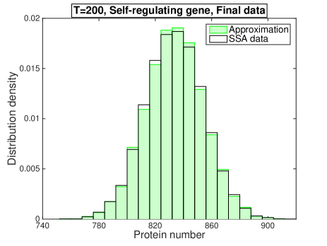
Figure 2: Histograms for the SSA data and for the approximation $h(W_{T})$ at time $T=200$.

The distributions of the protein numbers were determined at $t=50$ and $t=100$, and the corresponding histograms were plotted jointly with histograms for the SSA data as shown in Fig. 3.

\begin{overpic}[width=241.84842pt]{fig3a-eps-converted-to.pdf} \put(15.0,60.0){(a)} \end{overpic}

\begin{overpic}[width=241.84842pt]{fig3b-eps-converted-to.pdf} \put(15.0,60.0){(b)} \end{overpic}

Figure 3: Distributions of protein numbers for the self-regulating gene at $t=50$ (a) and $t=100$ (b) for the BSDE method and the SSA.

The means $\mu$ and the standard deviations $\sigma$ for the data obtained by the both methods are presented in Table 1. Although obtained by very different methods, the means and the standard deviations are in good agreement. The percent difference errors were computed as follows:

$${\rm Err}\,\mu=|(\mu_{\rm SSA}-\mu_{\rm BSDE})/\mu_{\rm SSA}|,$$

$${\rm Err}\,\sigma=|(\sigma_{\rm SSA}-\sigma_{\rm BSDE})/\sigma_{\rm SSA}|.$$

Table 1: The means $\mu$ and standard deviations $\sigma$ for the distribution of protein numbers for a self-regulating gene computed at $t=$ 0, 50, and 100. At $T=200$ we present $\mu$ and $\sigma$ obtained by using the final data approximation technique in comparison with the SSA data. The data obtained by the BSDE method are in the second and the third columns, and the data obtained by the SSA are in the fourth and the fifth columns. The last two columns present the percent difference errors.

	BSDE		SSA		$\%$Errors
Time	$\mu$	$\sigma$	$\mu$	$\sigma$	Err $\mu$	Err $\sigma$
0	500.75	0	500	0	0.15$\%$	–
50	587.13	10.99	586.44	10.53	0.11$\%$	4.35$\%$
100	671.37	15.30	670.78	14.78	0.08$\%$	3.51$\%$
200	833.80	20.46	833.27	20.52	0.06$\%$	0.31$\%$

Some trajectories of the BSDE solution $\eta_{t}$, representing the evolution of the number of proteins generated by a self-regulating gene, are shown in Fig. 4. This is an illustrative example of what the output of the BSDE method looks like, and how the trajectories of $\eta_{t}$ return to the same point which is close to $500$. This is a good approximation of the protein number that we used as the starting point for the SSA, and therefore, the prediction of this number by the BSDE method is very precise.

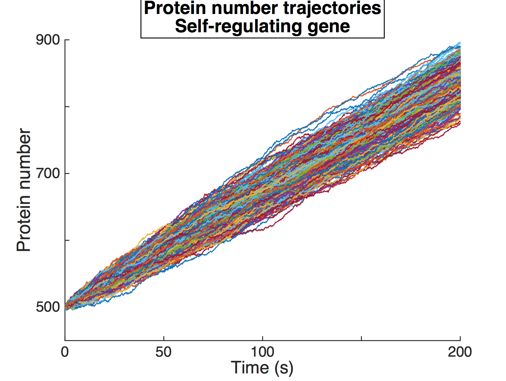
Figure 4: Trajectories of the stochastic process $\eta_{t}$, describing the protein number for the self-regulating gene, obtained by the BSDE method.

Networks of interacting genes.

In Figures 5 and 7 we show the distributions at $t=50$ and 100 for some genes of the networks of two and five genes, respectively.

\begin{overpic}[width=241.84842pt]{fig5a-eps-converted-to.pdf} \put(15.0,60.0){(a)} \end{overpic}

\begin{overpic}[width=241.84842pt]{fig5b-eps-converted-to.pdf} \put(15.0,60.0){(b)} \end{overpic}

Figure 5: Distributions of protein numbers at $t=50$ (a) and $t=100$ (b) for the 2nd gene of the network of two genes. The distributions are obtained by the BSDE method and the SSA.

\begin{overpic}[width=241.84842pt]{fig6a-eps-converted-to.pdf} \put(15.0,60.0){(a)} \end{overpic}

\begin{overpic}[width=241.84842pt]{fig6b-eps-converted-to.pdf} \put(15.0,60.0){(b)} \end{overpic}

Figure 6: Distributions of protein numbers at $t=50$ (a) and $t=100$ (b) for the 4th gene of the network of five genes. The distributions are obtained by the BSDE method and the SSA.

Also, we compare the means and the standard deviations at $t=50$ and 100 for the data obtained by the both methods. At final time $T=200$ we compare the means and the standard deviations obtained by the SSA and by our technique of final data approximation. The results are presented in Tables 2 and 3.

Table 2: The first four columns contain the means $\mu$ and the standard deviations $\sigma$ for the protein numbers of the network of 2 genes at $t=0$, $50$, and 100 obtained by the BSDE method and the SSA. At $T=200$ we present $\mu$ and $\sigma$ obtained by using the final data approximation technique in comparison with the SSA data. The last two columns conintain the percent difference errors.

Network of 2 genes
	BSDE		SSA		$\%$Errors
$t$	$\mu$	$\sigma$	$\mu$	$\sigma$	Err $\mu$	Err $\sigma$
1st gene
0	50.22	0	50.00	0	0.44$\%$	–
50	72.24	6.24	71.88	5.14	0.50$\%$	21.58$\%$
100	92.99	8.39	92.75	7.21	0.25$\%$	$16.41\%$
200	131.85	10.81	131.23	10.94	0.47$\%$	1.16$\%$
2nd gene
0	25.43	0	25.00	0	1.74$\%$	–
50	74.29	7.54	73.79	7.10	0.67$\%$	6.22$\%$
100	121.69	10.39	121.28	9.90	0.33$\%$	$4.93\%$
200	213.48	13.87	212.84	13.94	0.30$\%$	0.58$\%$

Table 3: The data representation is the same as in Table 2.

Network of 5 genes
	BSDE		SSA		$\%$Errors
$t$	$\mu$	$\sigma$	$\mu$	$\sigma$	Err $\mu$	Err $\sigma$
1st gene
0	50.80	0	50	0	1.61$\%$	–
50	72.70	5.75	71.90	5.19	1.11$\%$	10.78$\%$
100	93.54	7.72	92.86	7.19	0.73$\%$	$7.37\%$
200	132.23	9.89	131.73	9.92	0.38$\%$	0.32$\%$
2nd gene
0	25.51	0	25	0	2.04$\%$	–
50	74.25	7.52	73.78	7.14	0.63$\%$	5.31$\%$
100	121.79	10.35	121.39	9.93	0.33$\%$	$4.21\%$
200	213.42	13.94	212.92	13.98	0.23$\%$	0.28$\%$
3rd gene
0	10.58	0	10	0	5.83$\%$	–
50	58.82	7.77	58.31	6.98	0.89$\%$	11.27$\%$
100	104.72	10.43	104.16	9.86	0.53$\%$	$5.73\%$
200	189.94	13.36	189.43	13.39	0.27$\%$	0.28$\%$
4th gene
0	5.34	0	5	0	6.89$\%$	–
50	54.58	7.51	54.21	7.01	0.68$\%$	7.04$\%$
100	102.61	10.33	102.27	9.95	0.33$\%$	$3.81\%$
200	195.17	13.92	194.67	13.95	0.26$\%$	0.25$\%$
5th gene
0	50.66	0	50	0	1.32$\%$	–
50	72.57	5.72	71.99	5.19	0.80$\%$	10.24$\%$
100	93.41	7.69	92.89	7.21	0.55$\%$	$6.58\%$
200	132.12	9.84	131.61	9.87	0.38$\%$	0.31$\%$

Bistable network of two genes.

At timepoints $t=150$ and $t=200$ we compare the distributions with the SSA in the form of histograms (see Fig. 7). We observe a good agreement.

\begin{overpic}[width=241.84842pt]{fig7a-eps-converted-to.pdf} \put(15.0,60.0){(a)} \put(20.0,71.5){\framebox{{t=150, Bistability, 2nd gene}}} \end{overpic}

\begin{overpic}[width=241.84842pt]{fig7b-eps-converted-to.pdf} \put(15.0,60.0){(b)} \put(20.0,71.5){\framebox{{t=200, Bistability, 2nd gene}}} \end{overpic}

Figure 7: Distributions of protein numbers at $t=150$ (a) and $t=200$ (b) for the 2nd gene of the network of 2 genes for the bimodal distribution. The distributions are obtained by the BSDE method and the SSA.

Furthermore, we compare the values for initial protein numbers predicted by the FBSDE method with the actual initial protein numbers used in the SSA simulation. The BSDE simulation of the “blue” branch (Fig. 1) provides the initial number 103.83, while the BSDE simulating of the “red” branch provides the initial number 100.32 which are close to the initial number used in the SSA simution (which is 100). Similar results are obtained for the second gene. The results are presented in Table 4.

Table 4: The first line contains the data for initial protein numbers for the first gene. The value $\mu_{A}$ is obtained by a BSDE simulation of the “blue” branch, while $\mu_{B}$ is obtained by a BSDE simulation of the “red” branch. The second line contains the data for initial protein numbers for the second gene gene, the representation of the data is similar. The last two columns contain the percent difference errors.

Bistability in 2-genes networks
	BSDE		SSA	$\%$Errors
Gene	$\mu_{A}$	$\mu_{B}$	$\mu$	Err $\mu_{A}$	Err $\mu_{B}$
1st	103.83	100.32	100	3.83$\%$	0.32$\%$
2nd	50.36	50.78	50	0.71$\%$	1.55$\%$

Prediction of the initial value.

As we mentioned before, the BSDE method can be used to approximate the initial number of proteins. Since the solution to (1) can be represented as $\eta_{t}=\theta(t,W_{t})$, where $\theta$ is the solution to final value problem (2), then, as it is implied by the BSDE method, the initial protein number $\eta_{0}$ is deterministic and equals to $\theta(0,0)$. Tables 1–4, show that the BSDE method provides a good approximation for the initial number of proteins used as an initial condition in the SSA. The percent difference error is the biggest, $6,89\%$, when the initial number of proteins is $5$ (see Table 3), which is the smallest considered in our simulations. The percent difference error decreases when the initial protein number increases, and it equals to $0,15\%$ when we deal with large initial protein numbers as in the case of the self-regulating gene (see Table 1).

V Discussion

In this article we presented the BSDE method to model simple gene expression networks. As a backward method, it relies on the specification of a gene network model parametrization and on endpoint conditions (as opposed to initial conditions). It can therefore be applied when we know, or can measure, the distribution of proteins at a given time, and we want to determine the distributions at previous time points. In the BSDE method validation simulations, a good agreement was found between control and inferred protein level distributions, in terms of mean values and, in most cases, standard deviations. The BSDE method is therefore a powerful tool for time reversed simulations in gene networks / systems biology, where frequently an endpoint of interest is easily identifiable (and measured) and the aim is in assessing the prior (causal) conditions. Another advantage of our method is that it allows to determine, and even to simulate if necessary, the trajectory of the noise process. To our knowledge, the noise process is usually unknown and cannot be determined by any forward method. Obtaining the noise is the subject of our future work.

Determining the final condition.

The final condition for (1) is required to have the form $h(W_{T}),$ where $T$ is the fixed final time. In Section II.1, we described the construction of a piecewise linear function $h$ so that $h(W_{T})$ approximates a given final distribution provided by the SSA simulation. In practice, to obtain a distribution of protein amounts at time $T$, a large population of genetically identical cells is usually considered.

Diffusion process approximation.

We note that the stochastic process describing the protein number is an integer-valued pure-jump process which may change its values by $\pm 1$ at time, while the solution to (1) is a continuous process. However, assuming that the number of proteins of each type is sufficiently larger than 1, and the waiting times until the next synthesis or degradation are much smaller than the length of the interval $[t_{0},T]$, we can model the synthesis and degradation of proteins employing continuous diffusion processes, i.e. by BSDEs with Brownian drivers as (1). A diffusion process approximation for the dynamics of amounts of molecules was undertaken, for example, in Gillespie (2000); Chen et al. (2005); Raya and Desmond (2008).

Choice of rate functions.

We would like to emphasize that the choice of rate functions of form (10) is not important for the BSDE method to work. Although in our simulations we (as well as many other authors Mjolsness et al. (1991); Alon (2007); Das et al. (2010); Chen et al. (2009); Vu and Vohradsky (2006); Wang et al. (2007); Kim et al. (2013); Weaver et al. (1999)) used rate functions of form (10), the BSDE method works with any continuous function.

VI Appendix

BSDE versus SDE

One may think that BSDE (1) is equivalent to a usual (forward) SDE, since, similar to ODEs, knowing the final condition instead of the initial should lead to an equivalent problem. However, this is not the case if we require the solution to be adapted with respect to a Brownian motion (i.e. represented as a function of a Brownian motion). The requirement for the pair $(\eta_{t},z_{t})$ to be adapted implies that (under some additional analytical assumptions) BSDE (1) has a unique solution pair $(\eta_{t},z_{t})$ Pardoux and Pend (1990). Therefore, (1) is a different object than the traditional (forward) SDE. One may not be convinced why we should require from the solution $\eta_{t}$ to be adapted. Gillespie Gillespie (2000) proposed to model the dynamics of amounts of molecules changing during a chemical reaction by a forward SDE known as the Chemical Langevin Equation

$$\eta_{t}=\zeta+\int_{t_{0}}^{t}f(\eta_{s})\,ds+\int_{t_{0}}^{t}z_{s}\,dW_{s},$$

where $\zeta$ is the initial condition at time $t_{0}$. However, if $\eta_{t}$ solves this equation, the theory of SDEs implies that this solution is adapted. The process $z_{t}$ also must be adapted to ensure the existence of the stochastic integral. Therefore, the requirement for the solution pair $(\eta_{t},z_{t})$ to BSDE (1) to be adapted is a natural consequence of the Langevin dynamics. In this article, we propose to use a BSDE for modeling simple gene expression networks due to its property to have a pair of stochastic processes $(\eta_{t},z_{t})$ as the unique solution. The latter fact is important since the noise generating process $z_{t}$ is usually unknown.

References

- Thattai and van Oudenaarden (2001) M. Thattai and A. van Oudenaarden, Proc. Nat. Acad. Sci. 98, 8614 (2001).
- Ozbudak et al. (2002) E. Ozbudak, M. Thattai, I. Kurtser, A. Grossman, and A. van Oudenaarden, Nature Genetics 31, 69 (2002).
- Karlebach and Shamir (2008) G. Karlebach and R. Shamir, Nat. Rev. Mol. Cell Biol. 9, 770 (2008).
- Hecker et al. (2009) M. Hecker, S. Lambeck, S. Toepfer, E. van Someren, and R. Guthke, Biosystems 96, 86 (2009).
- Mettetal et al. (2006) J. Mettetal, D. Muzzey, J. Pedraza, E. Ozbudak, and A. van Oudenaarden, Proc. Nat. Acad. Sci. 103, 7304 (2006).
- Wilkinson (2011) D. Wilkinson, Bayesian Stat. 9, 679 (2011).
- Lillacci and Khammash (2013) G. Lillacci and M. Khammash, Bioinformatics 29, 2311 (2013).
- Gillespie (1977) D. Gillespie, J. Phys. Chem. 81, 2340 (1977).
- Bismut (1973) J. Bismut, J. Math. Anal. Appl. 44, 384 (1973).
- Pardoux and Pend (1990) E. Pardoux and S. Peng, Sys. Control Let. 14, 55 (1990).
- Ma et al. (1994) J. Ma, P. Protter, and Y. Yong, Probability Theory and Related Fields 98, 339 (1994).
- (12) “COPASI: Biochemical System Simulator,” http://copasi.org/.
- Mjolsness et al. (1991) E. Mjolsness, D. Sharp, and J. Reinitz, J. Theor. Biol. 152, 429 (1991).
- Alon (2007) U. Alon, Nat. Rev. Gen. 8, 450 (2007).
- Das et al. (2010) S. Das, D. Caragea, S. Welch, and W. H. Hsu, Handbook of research on computational methodologies in gene regulatory networks (IGI Global, 2010).
- Chen et al. (2009) L. Chen, R. Wang, and X. Zhang, Biomolecular networks: methods and applications in systems biology (Wiley, 2009).
- Vu and Vohradsky (2006) T. T. Vu and J. Vohradsky, Nucleic Acids Res. 35 (2006).
- Wang et al. (2007) H. Wang, L. Qian, and E. Dougherty, in Proc. 3rd International Conference on Natural Computation (2007).
- Kim et al. (2013) A. Kim, C. Martinez, J. Ionides, A. Ramos, M. Ludwig, N. Ogawa, D. Sharp, J. Reinitz, and M. Levine, PLoS Genetics 9 (2013).
- Weaver et al. (1999) D. Weaver, C. Workman, and G. Stromo, Pac. Symp. Biocomp. 4, 112 (1999).
- Gibson and Bruck (2000) M. A. Gibson and J. Bruck, in Computational modeling of genetic and biochemical networks, edited by J. M. Bower and H. Bolouri (MIT Press, 2000) pp. 49–72.
- Reinitz et al. (2003) J. Reinitz, S. Hou, and D. Sharp, ComPlexUs 1, 54 (2003).
- Hill (1910) A. V. Hill, J. Physiol. 40, IV (1910).
- Santillán (2008) M. Santillán, Math. Mod. Nat. Phenom. 3, 85 (2008).
- Bhaskaran et al. (2015) S. Bhaskaran, P. Umesh, and A. S. Nair, “Hill equation in modeling transcriptional regulation,” in Systems and Synthetic Biology, edited by V. Singh and P. K. Dhar (Springer, 2015) pp. 77–92.
- Gillespie (2000) D. Gillespie, J. Chem. Phys. 113, 297 (2000).
- Chen et al. (2005) K. Chen, T. Wang, H. Tseng, C. Huang, and C. Kao, Bioinformatics 21, 2883 (2005).
- Raya and Desmond (2008) K. Raya and J. Desmond, Theor. Comp. Sci. 408, 31 (2008).