Large Scale Anomalies in the Microwave Background: Causation and Correlation
Abstract
Most treatments of large scale anomalies in the microwave sky are a posteriori, with unquantified look-elsewhere effects. We contrast these with physical models of specific inhomogeneities in the early Universe which can generate these apparent anomalies. Physical models predict correlations between candidate anomalies and the corresponding signals in polarization and large scale structure, reducing the impact of cosmic variance. We compute the apparent spatial curvature associated with large-scale inhomogeneities and show that it is typically small, allowing for a self-consistent analysis. As an illustrative example we show that a single large plane wave inhomogeneity can contribute to low- mode alignment and odd-even asymmetry in the power spectra and the best-fit model accounts for a significant part of the claimed odd-even asymmetry. We argue that this approach can be generalized to provide a more quantitative assessment of potential large scale anomalies in the Universe.
Planck Ade et al. (2013a) and WMAP Bennett et al. (2013) yield independent, consistent maps of the cosmic microwave background (CMB). At large scales the main origin of uncertainty is the finite size of the visible Universe, rather than instrumental sensitivity or integrated observing time. Many CMB anomalies have been described Bennett et al. (2011); Ade et al. (2013b); Land and Magueijo (2005a); Tegmark et al. (2003); de Oliveira-Costa et al. (2004); Rakic and Schwarz (2007); Aslanyan et al. (2013a); Armendariz-Picon (2011); Aslanyan et al. (2013b); Land and Magueijo (2005b); Kim and Naselsky (2010); Gruppuso et al. (2011), including low- mode alignments or “axis of evil”, cold spot, hemispherical asymmetry, and parity asymmetry. These analyses are a posteriori and subject to large, unquantified “look-elsewhere” effects, and correlations between candidate anomalies are unknown. Further, values and similar tests are often used to assess the significance of anomalies Ade et al. (2013b), even though we cannot observe an ensemble of microwave skies.
By contrast, a physical mechanism that generates large-scale anisotropy will also predict the correlations between candidate anomalies, including those for which a search of our sky yields a null result, along with the associated polarization pattern. As an illustrative example, we analyze a model with a single amplified Fourier mode, showing this can generate low- mode alignments and parity asymmetry in the CMB Ade et al. (2013b). We compute the expected curvature generated by a large perturbation Bull and Kamionkowski (2013), finding that perturbations large enough to generate anomalies in the CMB do not also generate an apparent spatial curvature.
We work within the broad inflationary paradigm, but similar arguments could be made in other scenarios. Assume for simplicity that the perturbations have the Bunch-Davies form Baumann (2009), the Hubble parameter , and the spectral index . Single-field inflation Baumann (2009) with gauge-invariant curvature perturbations on uniform density hypersurfaces has the Mukhanov variable ,
| (1) |
where is the scale factor, is the inflaton, and is the slow-roll parameter. We quantize via
| (2) |
where and are the usual creation and annihilation operators, is the conformal time and
| (3) |
The mode functions satisfy the Mukhanov equation.
The Bunch-Davies vacuum state obeys
| (4) |
implying
| (5) |
At superhorizon scales the one- and two-point functions of the gauge-invariant curvature perturbation are
| (6) |
where denotes a value at horizon crossing. Now assume that some modes have particle content, for which the will differ from their vacuum values. For simplicity, consider a coherent state , i.e.
| (7) |
If at superhorizon scales the coherent Bunch-Davies states lead to identical two-point and three-point functions Kundu (2012). However, for a general coherent state
| (8) | |||||
| (9) |
One may think of as consisting of a quantum and a semiclassical piece Aslanyan et al. (2013b), and we treat as a semiclassical fluctuation where the are constrained by the data.
This scenario is a nonminimal model of inflation, in that the perturbations are not strictly Bunch-Davies. This is unsurprising, given that the purported anomalies are defined by their relatively low likelihood of being generated within the simplest models for the very early Universe. Given that this model is intended only as an illustrative example we do not provide a detailed mechanism for generating the additional perturbation. However, departures from Bunch-Davies will be common in models where the overall period of inflation is short and initial inhomegeneities are not fully erased.
Given we are interested in long wavelength curvature perturbations, we first ask whether these generate an effective spatial curvature within our Hubble volume if inflation starts at with the one-point function and when and we assume that currently observable modes were well inside the horizon at , or . The one-point functions (8) are approximately
| (10) |
When inflation begins , since is dimensionless in real space, and has units of , so
| (11) |
For superhorizon modes , and has the limit
| (12) |
Using the order-of-magnitude result, Eq. (11),
| (13) |
A mode crosses the horizon at . We define , a dimensionless measure of the perturbation at a scale
| (14) |
which vanishes in the limit that inflation has lasted for an arbitrarily long period.
Assuming rapid thermalization the Hubble parameter during inflation gives the density at the onset of radiation domination. The scale factor evolves from to during inflation and again taking and recalling that Baumann (2009), we find
| (15) |
and, at present,
| (16) |
where a subscript denotes a present-day value. We thus find a simple relationship between the present value of , the initial fluctuation amplitude , and the comoving scale . Furthermore, is proportional to and does not depend on the scale of inflation.
Recognizing , the curvature radius, in Eq. (16) we find
| (17) |
Large values of are incompatible with CMB data Aslanyan et al. (2013b) implying , so we are considering fluctuations with a wavelength much smaller than the curvature radius.
As a specific, illustrative example now consider a fluctuation in a single mode with the form
| (18) |
with when inflation starts. This scenario is discussed in Aslanyan et al. (2013b), which shows that for scales larger than where , the radius of the last scattering surface. Consequently, for this scenario . If at the onset of inflation we can inject fluctuations into the early Universe which match CMB anomalies and ensure that is compatible with current bounds, Ade et al. (2013a). This also serves as an estimate of the contribution of more complex anomalies, which could generically be decomposed in a superposition of plane waves, suggesting that generalizing the underlying ansatz would be consistent with the absence of any observed curvature.
Decomposing the linear fluctuation into spherical harmonics we find Aslanyan et al. (2013b)
| (19) |
where is the radiative transfer function for the corresponding mode ( or ). When the perturbation only appears on the even modes while for only odd modes are nonzero. Consequently, this scenario can lead to parity asymmetry in the CMB, a well-known candidate anomaly Ade et al. (2013b); Land and Magueijo (2005b); Kim and Naselsky (2010); Gruppuso et al. (2011); Liu et al. (2013).
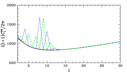
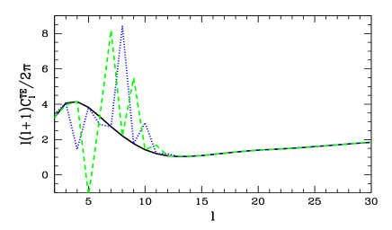
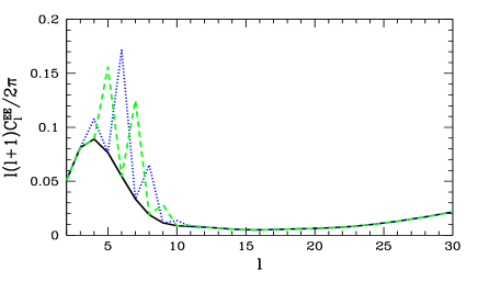
Purported anomalies in the temperature maps sourced by atypical primordial density fluctuations will be accompanied by a correlated anomaly in -mode polarization Dvorkin et al. (2008); Mortonson et al. (2009); Copi et al. (2013). Note that the polarization is not yet measured to the cosmic variance limit, so future polarization data will cross-check any physical model which was only constrained with temperature data.
We calculate the , , and power spectra for our simple model, showing the results in Fig. 1. The black solid curves show standard power spectra without any fluctuation, while the other two curves include a fluctuation with and wavelength . The blue dotted curve has and the green dashed curve has (our notation assumes that at our position).
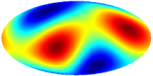
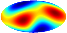
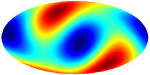
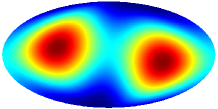
Our candidate inhomogeneity can also align low- modes in the CMB. The so-called “axis of evil” Ade et al. (2013b); Land and Magueijo (2005a); Tegmark et al. (2003); de Oliveira-Costa et al. (2004); Rakic and Schwarz (2007) is usually analyzed by finding the axis around which the angular momentum dispersion is maximized de Oliveira-Costa et al. (2004), where are the spherical harmonic coefficients in a coordinate system where the z axis has . From Eq. (19) one can show that for a single linear fluctuation the angular momentum dispersion is maximized around axes perpendicular to the direction of the fluctuation for all . Consequently, a single excited Fourier mode enhances the probability of multipole alignment. Moreover, for a fluctuation in two (nonparallel) Fourier modes the direction of maximum angular momentum dispersion will be given by the intersection of the corresponding planes. In Fig. 2 we show the quadrupole and the octupole for a simulated standard sky both without a fluctuation and with a sinusoidal fluctuation in the direction and the addition of the fluctuation pushes the otherwise random directions of the multipoles toward the plane perpendicular to .
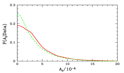
The power spectra are proportional to , so this signal is most efficiently constrained using the full likelihood function, which is sensitive to . This analysis was performed in Ref. Aslanyan et al. (2013b) using the WMAP temperature data. To estimate the improvement expected from Planck polarization data, we repeat that analysis with a simulated standard universe (no fluctuation added), but including polarization data, with Planck noise Planck Collaboration (2006) in the likelihood function. The posterior probability distribution for the amplitude is shown in Fig. 3. The solid red curve is obtained from temperature data only, the green dashed curve includes polarization data. The upper bound on is from temperature data only, with polarization data included.
Considering a simulated sky that includes a large scale fluctuation, we can assess the ability of polarization data to confirm the presence of the primordial inhomogeneity. A fluctuation just below the threshold of detectability, with (, ), yields an improvement in compared to the zero-amplitude case of from temperature data only, and with polarization data included. With the changes by with temperature only and with polarization included. Consequently, while polarization data does not significantly tighten a null result, it would be key to confirming an apparent detection.
The linear perturbation discussed here was fit to the WMAP7 data set in Ref. Aslanyan et al. (2013b). The best-fit and posterior probability distribution peaks near , , and , for the direction , and for this combination of and the power spectra have a strong odd-even asymmetry for small values of . As expected, the odd modes are enhanced compared to even modes since is close to and matches the conjectured direction of the odd-even asymmetry Ade et al. (2013b); Land and Magueijo (2005b); Kim and Naselsky (2010); Gruppuso et al. (2011). However, the best-fit direction is not close to being perpendicular to the axis of evil direction (, ) Ade et al. (2013b); Land and Magueijo (2005a); Tegmark et al. (2003); de Oliveira-Costa et al. (2004); Rakic and Schwarz (2007), so the best-fit fluctuation does not make a significant contribution to the mode alignment. However, for such that only odd or even modes are strongly enhanced only modes with a matching parity will be aligned. Consequently, to account for the observed mode alignment we would need more than one planar inhomogeneity.
Parameter estimation for a planar perturbation is computationally expensive Aslanyan et al. (2013b), and Bayesian evidence has not been computed for this scenario. However, for the best fit, improving the maximum likelihood by while adding 5 free parameters. The improved likelihood is restricted to a subregion of the overall parameter volume, suggesting that the marginalized likelihood is not significantly larger than that of CDM and the odds ratio is not significantly different from unity Jeffreys (1998). Consequently, the planar model is unlikely to be favored by Bayesian evidence, despite a nontrivial value associated with large scale parity violation.
Modifications to the primordial perturbations do not only affect the CMB, but also modify density fluctuations in the current epoch. The amplitude of the perturbation described by Eq. (18) is of the same order of magnitude as the usual quantum fluctuations, leading to signatures in large scale structure surveys that are potentially observable but which do not completely undermine global homogeneity. For the best-fit wavelength of , the density fluctuation varies from to its peak amplitude over , which maps a distance in redshift space of . Consequently, probes of large scale structure at such as the Planck SZ cluster catalogue Ade et al. (2013c) could further constrain the model.
Other observational consequences of a local density variation include the KSZ effect, Compton distortion Bull and Kamionkowski (2013); Valkenburg et al. (2013), and anisotropic cosmic expansion Kalus et al. (2013). For our model, matter density fluctuations at are of order , implying a similar variation in the spacetime metric and the expansion rate. This is within the current observational limit Bull and Kamionkowski (2013); Valkenburg et al. (2013); Kalus et al. (2013), although the detailed bounds were derived for models that differ from ours, so this is not a detailed comparison. However, it is clear that CMB anomalies generated by large scale inhomogeneities will have correlated signatures in large scale structure data, adding further discriminatory power to the approach described here.
In this Letter we contrast the a posteriori analysis of large scale anomalies in the microwave background with treatments based on a specific, physical model of the early Universe. In this case we have a causal model of the mechanism that underlies the anomaly and can examine correlations between observables and anomalies. We derived an order of magnitude estimate for the amplitude of induced by a large fluctuation and showed that large scale “anomalies” in the CMB need not also induce apparent spatial curvature. We analyzed correlations between temperature and polarization data for a simple model, and the ability of polarization data to confirm an apparent anomaly in the temperature maps. This specific model can explain the parity asymmetry of CMB without violating the flatness of the Universe at a detectable level.
Our results suggest that apparent anomalies in the microwave background can be usefully understood via the large scale fluctuations that might generate them. Moreover, anomalies in the microwave sky itself are effectively selected a posteriori from an infinite and ill-defined set of possible anomalies. Consequently these analyses suffer from a large and unquantified look-elsewhere effect which is not accounted for by values and similar frequentist statistics. By contrast, physical scenarios can be assessed in terms of their intrinsic credibility, described via systematic expansions, and tested using model selection tools.
We thank Eugene Lim, Aneesh Manohar, Hiranya Peiris, Layne Price, and Glenn Starkman for useful comments. The authors acknowledge the contribution of the NeSI high-performance computing facilities and the staff at the Centre for eResearch at the University of Auckland. New Zealand’s national facilities are provided by the New Zealand eScience Infrastructure (NeSI) and funded jointly by NeSI’s collaborator institutions and through the Ministry of Business, Innovation and Employment’s Infrastructure programme nes .
References
- Ade et al. (2013a) P. Ade et al. (Planck Collaboration), (2013a), arXiv:1303.5062 .
- Bennett et al. (2013) C. Bennett et al., Astrophys. J. Suppl. 208, 20 (2013).
- Bennett et al. (2011) C. Bennett et al., Astrophys .J. Suppl. 192, 17 (2011).
- Ade et al. (2013b) P. Ade et al. (Planck Collaboration), (2013b), arXiv:1303.5083 .
- Land and Magueijo (2005a) K. Land and J. Magueijo, Phys. Rev. Lett. 95, 071301 (2005a).
- Tegmark et al. (2003) M. Tegmark, A. de Oliveira-Costa, and A. J. S. Hamilton, Phys. Rev. D 68, 123523 (2003).
- de Oliveira-Costa et al. (2004) A. de Oliveira-Costa, M. Tegmark, M. Zaldarriaga, and A. Hamilton, Phys. Rev. D 69, 063516 (2004).
- Rakic and Schwarz (2007) A. Rakic and D. J. Schwarz, Phys. Rev. D 75, 103002 (2007).
- Aslanyan et al. (2013a) G. Aslanyan, A. V. Manohar, and A. P. S. Yadav, J. Cosmol. Astropart. Phys. 08, 009 (2013a).
- Armendariz-Picon (2011) C. Armendariz-Picon, J. Cosmol. Astropart. Phys. 03, 048 (2011).
- Aslanyan et al. (2013b) G. Aslanyan, A. V. Manohar, and A. P. S. Yadav, J. Cosmol. Astropart. Phys. 02, 040 (2013b).
- Land and Magueijo (2005b) K. Land and J. Magueijo, Phys. Rev. D 72, 101302 (2005b).
- Kim and Naselsky (2010) J. Kim and P. Naselsky, Astrophys. J. 714, L265 (2010).
- Gruppuso et al. (2011) A. Gruppuso et al., Mon. Not. R. Astron. Soc. 411, 1445 (2011).
- Bull and Kamionkowski (2013) P. Bull and M. Kamionkowski, Phys. Rev. D 87, 081301(R) (2013).
- Baumann (2009) D. Baumann, (2009), arXiv:0907.5424 .
- Kundu (2012) S. Kundu, J. Cosmol. Astropart. Phys. 02, 005 (2012).
- Liu et al. (2013) H. Liu, A. M. Frejsel, and P. Naselsky, J. Cosmol. Astropart. Phys. 07, 032 (2013).
- Dvorkin et al. (2008) C. Dvorkin, H. V. Peiris, and W. Hu, Phys. Rev. D 77, 063008 (2008).
- Mortonson et al. (2009) M. J. Mortonson, C. Dvorkin, H. V. Peiris, and W. Hu, Phys. Rev. D 79, 103519 (2009).
- Copi et al. (2013) C. J. Copi, D. Huterer, D. J. Schwarz, and G. D. Starkman, Mon. Not. R. Astron. Soc. 434, 3590 (2013).
- Planck Collaboration (2006) Planck Collaboration, (2006), arXiv:astro-ph/0604069 .
- Jeffreys (1998) H. Jeffreys, Theory of Probability, 3rd ed. (Oxford University Press, New York, 1998).
- Ade et al. (2013c) P. Ade et al. (Planck Collaboration), Astron. Astrophys. (to be published) (2013c), arXiv:1303.5089 .
- Valkenburg et al. (2013) W. Valkenburg, V. Marra, and C. Clarkson, Mon. Not. R. Astron. Soc. (to be published) (2013), arXiv:1209.4078 .
- Kalus et al. (2013) B. Kalus, D. J. Schwarz, M. Seikel, and A. Wiegand, Astron. Astrophys. 553, A56 (2013).
- (27) http://www.nesi.org.nz.