Elliptic flow from thermal photons with magnetic field in holography
Abstract
We compute the elliptic flow of thermal photons in a strongly coupled plasma with constant magnetic field via gauge/gravity duality. The D3/D7 embedding is applied to generate the contributions from massive quarks. By considering the cases in 2+1 flavor SYM analogous to the photon production in QGP, we obtain the thermal-photon , which is qualitatively consistent with the direct-photon measured in RHIC at intermediate energy. However, due to the simplified setup, the thermal-photon in our model should be regarded as the upper bound for the generated by solely magnetic field in the strongly coupled scenario.
The elliptic flow characterizes the momentum anisotropy of produced particles in heavy ion collisions. The recent observations from RHIC and LHC revealed surprising results, where the large elliptic flow of direct photons has been measuredAdare et al. (2012); Lohner (2012). Unlike the hadronic flow, the large flow of direct photons is unexpected since the high-energy photons are presumed to be generated in early times, where the initial flow should be relatively small compared to the flow built up by hydrodynamics. The anisotropy flow of thermal photons with viscous hydrodynamics has been recently reported in Dion et al. (2011); Shen et al. (2013). In theory, novel mechanisms should be introduced to break the azimuthal symmetry of photon production. The magnetic field led by colliding nuclei has been recently considered as one of possible candidates to bring about the large flow. In the weakly coupled scenario, the photon production with magnetic field has been studied in a variety of approachesTuchin (2011, 2012); Basar et al. (2012); Fukushima and Mameda (2012); Bzdak and Skokov (2013). Other mechanism such as the synchrotron radiation from the interaction of escaping quarks with the collective confining color field has been proposed in Goloviznin et al. (2012).
However, in the strongly coupled scenario, the perturbative approaches may not be applied. The AdS/CFT correspondenceMaldacena (1998); Witten (1998a); Gubser et al. (1998); Aharony et al. (2000); Witten (1998b), a holographic duality between a strongly coupled Super Yang-Mills(SYM) theory and a classical supergravity in the asymptotic background in the limit of large and strong t’Hooft coupling, is thus introduced to handle nonperturbative problems. Although the precise dual of QCD is unknown, the SYM and QCD may share same qualitative features in the strongly coupled regime at finite temperature. The thermal photon production from adjoint matters in the holographic dual was initiated by Caron-Huot et al. (2006) and then the one from fundamental matters was investigated in Mateos and Patino (2007). The relevant studies of thermal photons have been generalized to the QCD dualsParnachev and Sahakyan (2007); Jo and Sin (2011); Bu (2012) and the SYM duals with the intermediate couplingHassanain and Schvellinger (2012) or with pressure anisotropyRebhan and Steineder (2011); Patino and Trancanelli (2013). On the other hand, the computations of prompt photons and dileptons generated in early times via holography have been analyzed as wellBaier et al. (2012a, b); Steineder et al. (2012, 2013).
Motivated by the anomalous flow of direct photons in heavy ion collisions, the thermal photon production with constant magnetic field in holography have been studied Mamo (2012); Bu (2013); Yee (2013); Wu and Yang (2013); Arciniega et al. (2013). In Bu (2013), it is shown that the photon production perpendicular to the magnetic field in D3/D7 and D4/D6 embeddings with massless quarks is enhanced. In Yee (2013), the photon is computed in the framework of Sakai-Sugimoto modelSakai and Sugimoto (2005). The back reacted geometry in the presence of magnetic field may become anisotropic, which also results in an enhancement of photon productionArciniega et al. (2013). Furthermore, it is intriguing that the resonance in photon spectra from the meson-photon transition may lead to a mild peak of as pointed out in Wu and Yang (2013) when the photon production from massive quarks in D3/D7 embeddings is considered. To manifest the influence of the resonance on the elliptic flow, we will compute the of thermal photons in D3/D7 embeddings with constant magnetic field and incorporate the contributions from both massless and massive quarks.
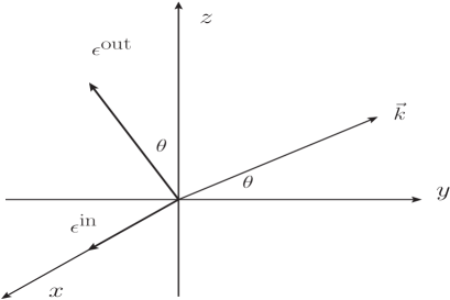
Our setup is illustrated in Fig.1, where the magnetic field is along the direction and two types of polarizations and are considered. The four momentum of photons is written as , where and . We will generalize the computations in the isotropic case of Wu and Yang (2013) to the photon production with arbitrary angle . We will take the quenched approximation by assuming , where denotes the number of flavors, and neglect the modification of flavor probe branes to the background geometry. The induced metric on D7 brane in the AdS-Schwarzschild background readsKarch and Katz (2002); Mateos et al. (2006); Hoyos-Badajoz et al. (2007)
where represents the radius of the internal wrapped by the D7 branes and denotes the blackening function for being the even horizon. Here we set the AdS radius . The temperature of the medium is determined by . For convenience, we will further set in computations. We then turn on the worldvolume U(1) gauge field coupled to the D7 branes, which generates constant magnetic field along the direction, where denotes the t’Hooft coupling. To further introduce the electromagnetic currents, we should perturb the D7 branes with worldvolume gauge fields. The relevant part of the DBI action now takes the form,
| (2) |
where is the worldvolume field strength from perturbation and is the D7-brane string tension for . In black hole embeddings corresponding to the deconfined phase, the field equation of in the DBI action with can be numerically solved by imposing the proper boundary conditions near the horizon Hoyos-Badajoz et al. (2007), and . The asymptotic solution of near the boundary behaves as
| (3) |
where the dimensionless coefficients and are related to the magnitudes of quark mass and condensate through Mateos et al. (2006, 2007)
| (4) | |||||
In the presence of gauge fields, the DBI action then gives rise to Maxwell equations
| (5) |
where the diagonal terms of the induced metric read
| (6) |
To compute the spectral functions, it is more convenient to convert the field equations into gauge invariant forms. For the in-plane polarization , the computation is straightforward. By taking in momentum space, we have to solve only one field equation,
| (7) |
where and . For the out-plane polarization , we have to consider coupled equations. By implementing the relation as shown in Fig.1, the field equations can be written into the gauge-invariant forms as
| (8) | |||||
where . The Maxwell equations in (7) and (8) can be solved numerically by imposing incoming-wave boundary conditions near the horizonCaron-Huot et al. (2006), where .
Since near the boundary, eq.(8) reduces to
| (9) |
By utilizing the relation above, the near-boundary action can be simplified as
| (10) |
where . We then evaluate the spectral density with the polarization via
| (11) | |||||
where denotes the retarded correlator. For the in-plane polarization, we have
| (12) | |||||
For the out-plane polarization, we have
where we utilize (9) to derive the second equality above. Solving the and for the out-plane polarization is more involved with the coupled equations, for which we discuss the technical details in the following. The procedure is similar to the computations in Patino and Trancanelli (2013).
Given that the out-plane solution is written in terms of the relevant bases as
| (14) |
where and , such bases should reduce to and on the boundary, which correspond to and in (Elliptic flow from thermal photons with magnetic field in holography). Since on the boundary, the bases follow the constraint . The task will be to find these relevant bases.
Presuming that and are two sets of incoming-wave solutions, the relevant bases should be formed by linear combinations of the them. We thus define
| (15) |
The bases on the boundary then read
| (16) |
where . By solving the coupled equations above, we find
| (17) |
where we set since the retarded correlators are invariant for an arbitrary . In practice, we could solve for two arbitrary incoming waves . Then by employing the coefficients shown in (Elliptic flow from thermal photons with magnetic field in holography) to recombine these two solutions, we are able to derive and for the out-plane polarization.
Finally, we may compute the elliptic flow for photon production. In the lab frame of heavy ion collisions, the four-momenta of photons can be parametrized as
| (18) |
where denote the rapidity and denote the transverse momentum perpendicular to the beam direction . Notice that at central rapidity, which reduces to our setup illustrated in Fig.1. The elliptic flow is defined as
| (19) |
where is the total yield of the emitted photons. In thermal equilibrium, the differential emission rate per unit volume is given by
| (20) |
In general, we have to take four dimensional spacetime integral of the emission rate to obtain the yield of photons. In our setup, where the medium is static, the spacetime integral leads to a constant volume, which is irrelevant for here. The elliptic flow at central rapidity hence becomes
| (21) |
All physical observables now will be scaled by temperature of the medium. We set , which corresponds to GeV2 in the regular scheme for and the average temperature of the SYM plasma MeV. In an alternative schemeGubser (2007), GeV2 for and MeV, where the temperature of SYM plasma is lower than that of QGP at fixed energy density. In heavy ion collisions, the approximated magnitude of magnetic field is about the hadronic scale, GeV2Tuchin (2013a). It turns out that the magnitude of magnetic field in the alternative scheme is close to the approximated value at RHIC. Even in the regular scheme, the magnitude of magnetic field in our model is not far from the approximated value. Hereafter we will make comparisons to QGP in the alternative scheme.
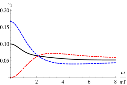
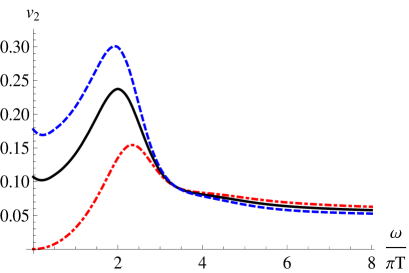
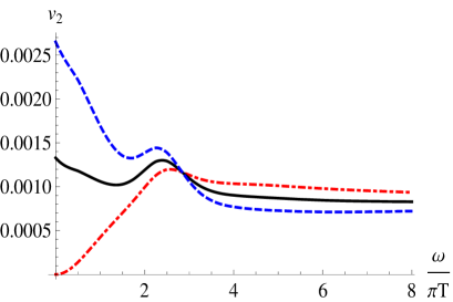
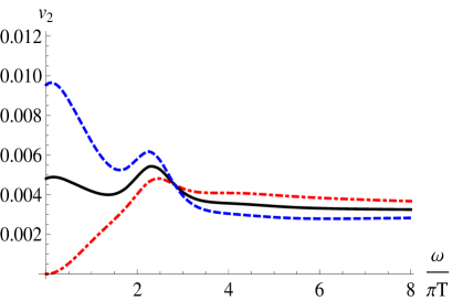
We firstly consider the elliptic flow contributed from massless quarks, which corresponds to the trivial embedding. As shown in Fig.2, the presence of magnetic field results in nonzero , while the remain featureless(without resonances). Here the averaged is obtained from the averaged emission rate of both the in-plane and out-plane polarizations. Whereas quarks may receive mass correction at finite temperature, we should consider the contributions from massive quarks as well. In addition, at intermediate energy, the photon spectra from the massive quarks may lead to resonances originated from the decays of heavy mesons to lightlike photonsMateos and Patino (2007); Casalderrey-Solana and Mateos (2009), which bring about considerable contribution to the spectra. As indicated in Wu and Yang (2013), the resonances in the presence of magnetic field depend on the moving directions of produced photons, which may generate prominent peaks in . To incorporate the massive quarks, we choose , which is close to the critical embedding. In fact, by further tuning up to one, the black hole embeddings may become unstable and multiple resonances will emerge in photon spectra similar to the scenarios in the absence of magnetic fieldMateos and Patino (2007). From (3), we find for the solution of the massive quarks, which corresponds to the bare quark mass MeV at the average RHIC temperature MeV in the alternative scheme. Due to the presence of magnetic field and the choice of the alternative scheme, the bare quark mass for the massive quark here is smaller than that in Mateos and Patino (2007); Casalderrey-Solana and Mateos (2009) to generate the resonance. As shown in Fig.3, a mild peak emerges at intermediate energy for the photon contributed from solely the massive quarks.
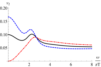
In analogy to the thermal photon production in QGP, we may consider scenario in the 2+1 flavor SYM plasma. We sum over the photon emission rates from two massless quarks and that from the massive quark with MeV to compute the . The results are shown in Fig.4, where the resonances of are milder. In QGP, the regime in which the thermal photons make substantial contributions is around GeV at central rapidity, where denotes the transverse momentum of direct photons. By rescaling with , such a regime corresponds to in Fig.4 at MeV. It turns out that the in our holographic model resemble the RHIC data for the flow of direct photons at intermediate Adare et al. (2012). Although the mass of the massive quark in our setup does not match that of the strange quark, the mass we introduce is not far from the scale of strange mesons. The resonances in our setup may suggest the transitions of strange mesons to photons in QGP in the presence of magnetic field. On the other hand, the resonance of coming from meson-photon transitions may not be subject to the strongly coupled scenario. In the weakly coupled approach such as Basar et al. (2012), where the finite-temperature corrections to the intermediate meson in the effective coupling is not considered, the photon production perpendicular to the magnetic field can be possibly enhanced provided that the thermal dispersion relation of the intermediate meson becomes lightlike.
Finally, we mention the caveats when making comparisons between our holographic model and heavy ion collisions in reality except for the intrinsic difference between SYM theory and QCD. Firstly, the QGP undergoes time-dependent expansion, while the medium in our model is static in thermal equilibrium. Second, the magnetic field produced by colliding nuclei is time-dependent, which decay rapidly in early times. Although the influence of thermal quarks on the lifetime of magnetic field is controversialTuchin (2013a); McLerran and Skokov (2013); Tuchin (2013b), the constant magnetic field in our model could overestimate the flow. According to Tuchin (2013a), the magnetic field decreases by a factor of between the initial (0.1 fm/c)and final (5 fm/c) times in the presence of nonzero conductivity. As a simple approximation, we may assume that the magnetic field is described by a power-law drop-off, which results in . By taking the initial and freeze-out temperature as MeV and MeV, we find the freeze-out time fm as we set the thermalization time fm and average temperature MeV with the Bjorken hydrodynamics . We than obtain the average magnetic field with the setup above, where is the initial magnetic field. By utilizing the average magnetic field with the same t’Hooft coupling and average temperature, we find that the drop about times as shown in Fig.5.
Although the photon here can only be evaluated numerically, it is approximately proportional to for small . As a result, we may as well consider the result with average . With the above approximation, we find corresponding to . As shown in Fig.6, the with drop times. However, as the nonlinear effect with large becomes more pronounced, the computation with average magnetic field may underestimate the contribution from such strong magnetic field in early times. It is thus desirable to incorporate time-dependent magnetic field in the setup as future work. On the other hand, it is also worthwhile to notice that the in our model is enhanced as we turn down the coupling with fixed magnetic field and temperature through the relation .
Since we choose the maximum magnetic field from its initial value, the obtained in our model should be regarded as the upper bound generated by solely magnetic field in the strongly coupled scenario. In reality, such a mechanism only yields partial contribution of the measured . As shown in Shen et al. (2013), the viscous hydrodynamics also results in a substantial contribution to thermal-photon . To construct full for thermal photons, both contributions from magnetic field and from viscous hydrodynamics should be taken into account. Furthermore, in the alternative scheme, the intermediate t’Hooft coupling is taken, where the corrections from finite t’Hooft coupling in the gravity dual have to be considered. More explicitly, the next leading order correction is of . It is found in Hassanain and Schvellinger (2012) that the photoemission rate increases as the coupling decreases in the absence of magnetic field when the correction is included.
The authors thank S. Cao and G. Qin for useful discussions. This material is based upon work supported by DOE grants DE-FG02-05ER41367 (B. Müller and D. L. Yang), the National Science Council (NSC 101-2811-M-009-015) and the Nation Center for Theoretical Science(102-2112-M-033-003-MY4), Taiwan (S. Y. Wu).
References
- Adare et al. (2012) A. Adare et al. (PHENIX Collaboration), Phys.Rev.Lett. 109, 122302 (2012), eprint 1105.4126.
- Lohner (2012) D. Lohner (ALICE Collaboration) (2012), eprint 1212.3995.
- Dion et al. (2011) M. Dion, J.-F. Paquet, B. Schenke, C. Young, S. Jeon, et al., Phys.Rev. C84, 064901 (2011), eprint 1109.4405.
- Shen et al. (2013) C. Shen, U. W. Heinz, J.-F. Paquet, I. Kozlov, and C. Gale (2013), eprint 1308.2111.
- Tuchin (2011) K. Tuchin, Phys.Rev. C83, 017901 (2011), eprint 1008.1604.
- Tuchin (2012) K. Tuchin (2012), eprint 1206.0485.
- Basar et al. (2012) G. Basar, D. Kharzeev, D. Kharzeev, and V. Skokov, Phys.Rev.Lett. 109, 202303 (2012), eprint 1206.1334.
- Fukushima and Mameda (2012) K. Fukushima and K. Mameda, Phys.Rev. D86, 071501 (2012), eprint 1206.3128.
- Bzdak and Skokov (2013) A. Bzdak and V. Skokov, Phys.Rev.Lett. 110, 192301 (2013), eprint 1208.5502.
- Goloviznin et al. (2012) V. Goloviznin, A. Snigirev, and G. Zinovjev (2012), eprint 1209.2380.
- Maldacena (1998) J. M. Maldacena, Adv.Theor.Math.Phys. 2, 231 (1998), eprint hep-th/9711200.
- Witten (1998a) E. Witten, Adv.Theor.Math.Phys. 2, 253 (1998a), eprint hep-th/9802150.
- Gubser et al. (1998) S. Gubser, I. R. Klebanov, and A. M. Polyakov, Phys.Lett. B428, 105 (1998), eprint hep-th/9802109.
- Aharony et al. (2000) O. Aharony, S. S. Gubser, J. M. Maldacena, H. Ooguri, and Y. Oz, Phys.Rept. 323, 183 (2000), eprint hep-th/9905111.
- Witten (1998b) E. Witten, Adv.Theor.Math.Phys. 2, 505 (1998b), eprint hep-th/9803131.
- Caron-Huot et al. (2006) S. Caron-Huot, P. Kovtun, G. D. Moore, A. Starinets, and L. G. Yaffe, JHEP 0612, 015 (2006), eprint hep-th/0607237.
- Mateos and Patino (2007) D. Mateos and L. Patino, JHEP 0711, 025 (2007), eprint 0709.2168.
- Parnachev and Sahakyan (2007) A. Parnachev and D. A. Sahakyan, Nucl.Phys. B768, 177 (2007), eprint hep-th/0610247.
- Jo and Sin (2011) K. Jo and S.-J. Sin, Phys.Rev. D83, 026004 (2011), eprint 1005.0200.
- Bu (2012) Y. Y. Bu, Phys. Rev. D 86, 026003 (2012), URL http://link.aps.org/doi/10.1103/PhysRevD.86.026003.
- Hassanain and Schvellinger (2012) B. Hassanain and M. Schvellinger, Phys.Rev. D85, 086007 (2012), eprint 1110.0526.
- Rebhan and Steineder (2011) A. Rebhan and D. Steineder, JHEP 1108, 153 (2011), eprint 1106.3539.
- Patino and Trancanelli (2013) L. Patino and D. Trancanelli, JHEP 1302, 154 (2013), eprint 1211.2199.
- Baier et al. (2012a) R. Baier, S. A. Stricker, O. Taanila, and A. Vuorinen, JHEP 1207, 094 (2012a), eprint 1205.2998.
- Baier et al. (2012b) R. Baier, S. A. Stricker, O. Taanila, and A. Vuorinen (2012b), eprint 1207.1116.
- Steineder et al. (2012) D. Steineder, S. A. Stricker, and A. Vuorinen (2012), eprint 1209.0291.
- Steineder et al. (2013) D. Steineder, S. A. Stricker, and A. Vuorinen (2013), eprint 1304.3404.
- Mamo (2012) K. A. Mamo (2012), eprint 1210.7428.
- Bu (2013) Y. Bu, Phys. Rev. D 87, 026005 (2013), URL http://link.aps.org/doi/10.1103/PhysRevD.87.026005.
- Yee (2013) H.-U. Yee, Phys.Rev. D88, 026001 (2013), eprint 1303.3571.
- Wu and Yang (2013) S.-Y. Wu and D.-L. Yang, JHEP 1308, 032 (2013), eprint 1305.5509.
- Arciniega et al. (2013) G. Arciniega, P. Ortega, and L. Patino (2013), eprint 1307.1153.
- Sakai and Sugimoto (2005) T. Sakai and S. Sugimoto, Prog.Theor.Phys. 113, 843 (2005), eprint hep-th/0412141.
- Karch and Katz (2002) A. Karch and E. Katz, JHEP 0206, 043 (2002), eprint hep-th/0205236.
- Mateos et al. (2006) D. Mateos, R. C. Myers, and R. M. Thomson, Phys.Rev.Lett. 97, 091601 (2006), eprint hep-th/0605046.
- Hoyos-Badajoz et al. (2007) C. Hoyos-Badajoz, K. Landsteiner, and S. Montero, JHEP 0704, 031 (2007), eprint hep-th/0612169.
- Mateos et al. (2007) D. Mateos, R. C. Myers, and R. M. Thomson, JHEP 0705, 067 (2007), eprint hep-th/0701132.
- Gubser (2007) S. S. Gubser, Phys.Rev. D76, 126003 (2007), eprint hep-th/0611272.
- Tuchin (2013a) K. Tuchin (2013a), eprint 1301.0099.
- Casalderrey-Solana and Mateos (2009) J. Casalderrey-Solana and D. Mateos, Phys.Rev.Lett. 102, 192302 (2009), eprint 0806.4172.
- McLerran and Skokov (2013) L. McLerran and V. Skokov (2013), eprint 1305.0774.
- Tuchin (2013b) K. Tuchin (2013b), eprint 1305.5806.