Interface limited growth of heterogeneously nucleated ice in supercooled water

Abstract

Heterogeneous ice growth exhibits a maximum in freezing rate arising from the competition between kinetics and the thermodynamic driving force between the solid and liquid states. Here, we use molecular dynamics simulations to elucidate the atomistic details of this competition, focusing on water properties in the interfacial region along the secondary prismatic direction. The crystal growth velocity is maximized when the efficiency of converting interfacial water molecules to ice, collectively known as the attachment kinetics, is greatest. We find water molecules that contact the intermediate ice layer in concave regions along the atomistically roughened surface are more likely to freeze directly. An increased roughening of the solid surface at large undercoolings consequently plays an important limiting role on the rate of ice growth, as water molecules are unable to integrate into increasingly deeper surface pockets. These results provide insights into the molecular mechanisms for self-assembly of solid phases that are important in many biological and atmospheric processes.

I Introduction

Self-assembly of a disordered liquid to an ordered solid is one of the most basic physical processes that occurs in nature. Kirkpatrick (1975); Levi and Kotrla (1997) Of these processes, the homogenous and heterogeneous growth of ice from liquid water has attracted considerable attention due to its relevance in atmospheric physics, Petrenko and Whitworth (2002); Koop et al. (2000); Murray et al. (2005); Murphy and Koop (2005); Cantrell and Heymsfield (2005) cryobiology, Mazur (1963, 1970) and in the antifreeze and food preservation industries. Griffith and Ewart (1995); Feeney and Yeh (1998); Carvajal-Rondanelli et al. (2011); Hassas-Roudsari and Goff (2012) However, while the thermodynamics of freezing is largely understood, Libbrecht (2005); Bartels-Rausch et al. (2012) the molecular details of the freezing process are less well established.

Owing to the constantly evolving nature of ice growth, it is difficult to probe the moving solid-liquid interfacial region experimentally at the microscopic level. Measurements have shown the ice-water interface to be on the order of $\sim 1$ nm wide, or three water layers thick, near equilibrium at the melting temperature. Beaglehole and Wilson (1993) Experiments observing dendritic ice growth have measured maximum growth rates on the order of $10$ cm/s for the basal plane at temperatures $\Delta T_{{\rm M}}=-18$ K below the melting point. Pruppacher (1967); Langer et al. (1978); Furukawa and Shimada (1993) Experimental deviations of growth rates from theoretical predictions Shibkov et al. (2005) were suggested to be due to an unaccounted-for competition between collective molecular attachment (freezing) and detachment (melting) processes near the solid surface. Wilson (1900); Frenkel (1932); Kolmogorov (1937); Johnsson and Mehl (1940); Avrami (1940); Shibkov et al. (2005)

Molecular dynamics (MD) simulations have proved a useful tool for probing the microscopic properties of the (moving) solid-liquid interface more directly. Karim and Haymet (1987); Karim O. A. Haymet (1988); Nada and Furukawa (1995); Baéz and Clancy (1995); Hayward and Haymet (2001, 2002); Nada and Furukawa (2005); Carignano et al. (2005); Kim and Yethiraj (2008); Kim et al. (2009); Pirzadeh and Kusalik (2010); Rozmanov and Kusalik (2011); Pirzadeh et al. (2012); Seo et al. (2012); Rozmanov and Kusalik (2012a, b); Moore and Molinero (2011); Shepherd et al. (2012) These studies have also shown the interfacial region is about three water layers wide, and consists of a slushy mix of ice and liquid features whose dynamical properties are greatly arrested compared to the bulk liquid. Hayward and Haymet (2001); Carignano et al. (2005) Ice growth rates were shown to reach a maximum deep within the supercooled regime, initially increasing as the temperature was lowered below the melting point, but then decreasing upon further undercooling below a characteristic temperature. Rozmanov and Kusalik (2011); Weiss et al. (2011); Moore and Molinero (2011) Ideally, one would like to establish how the structure, shape, dynamics, and molecular attachment rates at the ice surface change with external conditions near this crossover point. If the self-assembly mechanism is a competition between the rates of attachment and detachment at the liquid-solid contact, what microscopic properties at the interface favor molecular retention or loss? Furthermore, what microscopic properties explain why the freezing rate reaches a maximum in the supercooled regime?

Here, we use molecular dynamics simulations to investigate how temperature affects the attachment kinetics of water to the secondary prismatic face of ice I_h. We find the temperature dependence of the ice growth rate reaches a maximum when the microscopic efficiency of converting interfacial water to ice is maximum. This efficiency is limited at higher temperatures due to repeated melting and surface migration Rost et al. (2003) events across the interfacial regions. At lower temperatures, the interplay between the roughening of the ice surface and increased tetrahedrality of the liquid Moore and Molinero (2011) play important limiting roles. We find molecules which make contact with the intermediate ice layer in concave regions are more likely to freeze directly. Molecules that make contact with regions of higher curvature tend to escape back into the liquid. Consequently, water molecules are unable to rearrange and fit into to increasingly deeper surface pockets at very low temperatures. Our results highlight the important role played by interfacial water properties in determining the rate of heterogeneous ice growth at increasingly larger undercoolings.

II Simulations Details

Molecular dynamics simulations of the TIP4P/2005 water model Abascal and Vega (2005) were performed using the GROMACSHess et al. (2008) package on the ice-liquid system shown in Fig. 1a under isobaric-isothermal conditions. Periodic boundary conditions were employed with the long range electrostatics treated using particle-mesh Ewald summation. Essmann et al. (1995) The pressure was kept at 1 bar using an anisotropic Parrinello-Rahman Parrinello and Rahman (1981) barostat with a time constants of 10 ps. Constant temperature conditions were imposed using a Langevin thermostat with a time constant of 4.0 ps, which quickly removes latent heat from the system. Weiss et al. (2011); Rozmanov and Kusalik (2011) Thermostat couplings from 0.1 to 100.0 ps did not affect the observed freezing rates at $240$ K within statistical error.

Water intermolecular interactions were modeled using the fully-atomistic TIP4P/2005 potential. This model was chosen since it has been shown to accurately reproduce the high density phase diagram of water and ice, Abascal and Vega (2005) as well as the dynamics of water in the supercooled regime. Stirnemann and Laage (2012) The melting temperature of the model is $250$ K, Fernández et al. (2006) which is considerably more accurate compared with other simple point charge water potentials given the other advantages of this model. Freezing rates obtained with the model are also close to experimentally observed values. Rozmanov and Kusalik (2011)

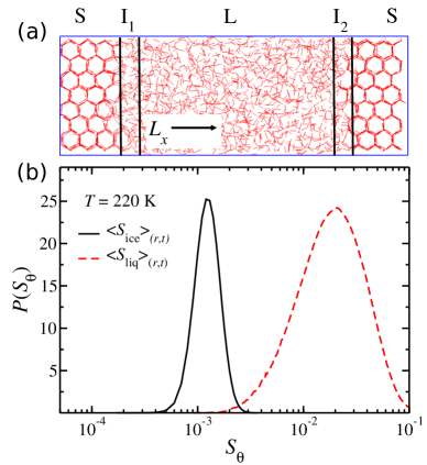
Figure 1: (a) Initial configuration used in the simulations with schematic outlines of the two interfacial regions (I₁, I₂) separating the solid (S) and liquid (L) phases. Ice grows along the $L_{x}$-direction. (b) Tetrahedral order parameter distributions where angle brackets $\langle S\rangle_{(r,t)}$ denote both spatial averaging over several configurations of the trajectory, as well as time-based (exponential) smoothing of the resultant instantaneous order parameters for each molecule in separate bulk ice and liquid simulations. Overlap between ice and liquid distributions is significantly reduced using this scheme. The ice distribution is normalized by $1/45$ to make the y-axis scale more tractable for viewing.

The initial ice structure was prepared according to the Bernal-Fowler rules, Bernal and Fowler (1933) and brought in contact with an amorphous water configuration approximately three times the thickness of the ice region. The secondary prismatic plane of ice was chosen to contact the water region since it is the fastest growing face of ice. Rozmanov and Kusalik (2011) The resulting configuration consisted of a sheet of ice (S) and bulk liquid (L) separated by two ice-liquid interfacial regions (I₁, I₂) shown schematically by the vertical lines in Fig. 1a. Ice growth was monitored perpendicular to the interface along the $L_{x}$ direction. Two system sizes were used to assess finite size effects. Ten trajectories at each temperature were performed using a small simulation cell containing 2696 water molecules with approximate dimensions 9.1 nm $\times$ 3.1 nm $\times$ 2.9 nm. Additionally, three trajectories were performed at each temperature using a large simulation cell, which had nine times the cross-sectional surface area of the small system and contained 24,264 water molecules. Data was only gathered until each trajectory was 60% frozen. This ensured that the close proximity of the two interfacial regions in the simulations cell did not affect the analysis at longer times.

III Interface identification

We developed a robust scheme for classifying the evolving ice, liquid, and interfacial regions throughout the freezing process. This classification was accomplished by employing a suitable order parameter to distinguish between local ice- and liquid-like structure, and then using profile functions of this order parameter to identify the instantaneous interface as described below.

III.1 Instantaneous molecule classification

We used a local tetrahedral order parameter to classify whether the local structure about a water molecule was ice- or liquid-like, Chau and Hardwick (1998)

$$S_{\theta}=\frac{3}{32}\sum_{j=1}^{3}\sum_{k=j+1}^{4}\left(\cos\theta_{jk}+\frac{1}{3}\right)^{2}\,$$ (1)

where the summations extended over all hydrogen bond angles $\theta_{jk}$ defined by the nearest four neighboring oxygen atoms around a given molecule. To enhance our ability to distinguish between ice- and liquid-like distributions (which can overlap up to 20% at low temperatures), we used a combination of position averaging and exponential time smoothing of the trajectories as described in Appendix A. A water molecule was labeled as ice-like when its resultant order parameter $\langle S_{\theta}\rangle_{t}$ was less than a carefully selected threshold criteria $S_{{\rm tol}}$. Using the smoothing procedure, near perfect separation between ice and liquid configurations can be obtained with less than 4% overlap between bulk ice and bulk liquid distributions at $220$ K, as shown in Fig. 1b. The critical threshold value were chosen to be $S_{{\rm tol}}=0.002$ for $220$ K, and $S_{{\rm tol}}=0.005$ for all other temperatures. At $300$ K, no water molecules were misclassified as ice-like in simulations of the bulk liquid. All other observables were calculated from the raw unaveraged trajectories.

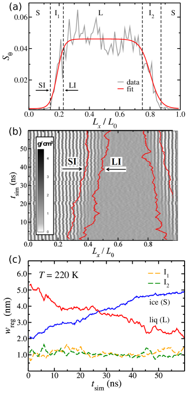
Figure 2: (a) Tetrahedral order parameter binned along direction of ice growth and resultant profile function used to identify the solid-interface (SI) and liquid-interface (LI) dividing surfaces. (b) Contour map of the density profile evolving during a typical trajectory with the solid lines giving the instantaneous interfacial boundaries (SI and LI) for each interfacial region. (c) Average resultant thicknesses of the ice, liquid, and the widths $w_{{\rm reg}}$ of the interfacial regions (I₁, I₂).

III.2 Instantaneous interface classification

The instantaneous positions of the interfacial regions were identified from profile functions of the tetrahedral order parameter $\langle S_{\theta}\rangle_{t}$ projected along the direction of ice growth. This approach is similar to methods used in previous studies to define the extent of the interfacial region. Karim and Haymet (1987); Hayward and Haymet (2001); Razul and Kusalik (2011) Here, we track two interface boundaries as shown in Fig. 2a: the solid-interface (SI) and the liquid-interface (LI). These dividing surfaces (dashed vertical lines in the figure) were identified using the procedure described in Appendix B.

Fig. 2b shows the projected density along the scaled simulation box for a typical trajectory at $220$ K obtained using this scheme. From these boundary lines, the widths of the interfacial regions (I₁, I₂), and the thicknesses of the ice (S) and liquid (L) regions can be monitored as freezing occurs, as shown in Fig. 2c. Importantly, the interfacial widths remain roughly constant throughout the simulation, and are on the order of $\sim 1$ nm, or approximately three water layers, consistent with experimental measurements Beaglehole and Wilson (1993) and other MD studies. Hayward and Haymet (2001); Razul and Kusalik (2011); Pirzadeh et al. (2012); Shepherd et al. (2012)

Since ice growth does not proceed on a layer-by-layer basis along the prismatic directions, Nada and Furukawa (1995); Carignano et al. (2005); Seo et al. (2012) we modeled the rough SI and LI surfaces by dividing the cross-sectional area of the simulation box into a 2D array of fibers extending the entire length of the system along the direction of ice growth. Each square fiber was defined by a feature size of $d_{{\rm f}}=0.6$ nm sides. The envelope functions, and subsequently the positions of the SI and LI boundaries, were formed separately in each fiber.

IV Results and discussion

IV.1 Growth rate maximum

The measured ice growth rates $R_{{\rm G}}$ along the secondary prismatic direction for different temperatures is shown in Fig. 3a. The growth rate profile reaches a maximum of $9.6\pm 0.5$ cm/s at $240$ K ($\Delta T_{{\rm M}}=-10$ K), in good agreement with previous results using this water model. Rozmanov and Kusalik (2012b) Experimental studies of the growth of ice dendrites report growth velocities of 10-12 cm/s for the fastest growing ice faces at temperatures $\Delta T_{{\rm M}}=-18$ K below the melting point. Pruppacher (1967); Bauerecker et al. (2008)

The maximum in the growth rate in Fig. 3a is characteristic of a crossover from thermodynamically-driven to kinetic-limited crystal growth. Kirkpatrick (1975); Moore and Molinero (2011); Rozmanov and Kusalik (2011); Weiss et al. (2011) From $247$ to $240$ K, the rate of crystal growth increases by a factor of $\sim 2$ as the chemical potential difference between the liquid and solid phases increases (i.e. $\mu_{{\rm L}}-\mu_{{\rm S}}>0$) and ice becomes thermodynamically more favorable. Bartels-Rausch et al. (2012) Below $240$ K, the growth rate progressively decreases and is a factor of $\sim 5$ smaller at $220$ K than the maximum. This decrease is described as arising from increasing kinetic barriers governing activated processes such as diffusion, which become rate-limiting below $240$ K. Kirkpatrick (1975); Rozmanov and Kusalik (2011) We note the lowest temperature $220$ K is below where the peak in the isobaric heat capacity occurs for this water model ($\sim 225$ K – which signifies the onset of water’s so called no-man’s land), Mishima and Stanley (1998); Moore and Molinero (2010); Abascal and Vega (2010); Malaspina et al. (2013) and was included to see if the scaling of the growth process continues as the system enters this deeply cooled regime.

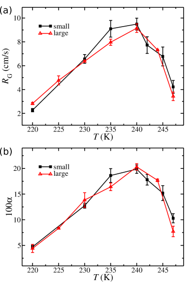
Figure 3: (a) Average crystal growth velocities $R_{{\rm G}}$ for the secondary prismatic face of ice I_h for the two system sizes. (b) The retention probability $\alpha$ defining the system efficiency of converting liquid water molecules to ice.

To assess the efficiency with which water molecules in the interfacial regions are incorporated into the ice phase at the varying temperatures, we consider the interfacial retention probability $\alpha$,

$$\alpha=\frac{\Phi_{{\rm F}}}{\Phi_{{\rm F}}+\Phi_{\rm E}}\,,$$ (2)

where $\Phi_{{\rm F}}$ is the flux (number of molecules per nm² per ns) of liquid molecules that irreversibly freeze to the solid surface, and $\Phi_{{\rm E}}$ is the flux of liquid molecules that enter the interfacial region but later escape to the liquid without freezing. Written in this way, $\alpha$ is the liquid-to-ice conversion efficiency of the system, or the percentage of water molecules that freeze from the total number of water molecules that cross into the interfacial regions (I₁ and I₂) from the liquid.

The temperature dependence of the retention probability $\alpha$ in Fig. 3b follows the same trend observed in the growth rate profile, exhibiting a maximum at $240$ K and minima at the lowest and highest temperatures $220$ and $247$ K for both system sizes studied. This temperature dependence is intuitively expected since the crystal growth velocity is microscopically determined by the rates which molecules become incorporated into the solid surface. Crystal growth will be limited if the conversion of liquid molecules to ice is low, as is the case at $220$ and $247$ K in Fig. 3b.

The individual contributions to the retention probability in Fig. 4 allow the origins of the freezing efficiency to be assessed. As can be seen from Fig. 4a, the flux of molecules that irreversibly freeze $\Phi_{\rm F}$ increases by nearly a factor of $\sim 2$ as the temperature is lowered from $247-240$ K and ice becomes thermodynamically more favorable. There are fewer irreversible freeze events at $247$ K because of an increased propensity to melt, or to detach from the ice-like layers near the solid surface (see next paragraph), which is intuitively expected near the melting point. Below $240$ K, however, $\Phi_{\rm F}$ begins to decrease significantly from its maximum value, by up to a factor of $\sim 4$ at $220$ K (a similar change in freezing rate is observed in Fig. 3a). While the increased tetrahedrality of the liquid Moore and Molinero (2011) and corresponding slow-down in water dynamics Weiss et al. (2011) are expected to contribute to the observed decrease in freeze events, we examine further below how changes in the interfacial structure can also play a limiting role on the attachment kinetics at low temperatures.

The escape flux of molecules that enter the interfacial region but return to the liquid is shown in Fig. 4b. The nonmonotonic behavior shows that the number of escape events is (somewhat unintuitively) greater at both $220$ and $247$ K. An increased propensity to detach from the ice surface (or ice-like layers near the ice surface), plays an increasingly greater contribution to the escape flux as the temperature increases. Fig. 4c shows how the flux $\Phi_{{\rm M}}$ of frozen molecules that detach from the ice and ice-like planes near the solid surface, i.e. melt events, increases with temperature and proximity to the liquid region (dashed lines), as is intuitively expected. At temperatures below $240$ K, however, increasing values for $\Phi_{{\rm E}}$ are more puzzling. This greater propensity to return to the liquid will be attributed to a roughening of the intermediate ice layers, as will be discussed further below.

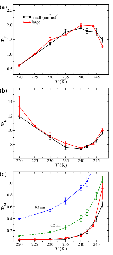
Figure 4: (a) The flux $\Phi_{{\rm F}}$ of molecules that irreversibly freeze to the solid phase. (b) The flux $\Phi_{{\rm E}}$ of molecules that cross into the interfacial regions but later escape to the liquid without contacting the ice surface. (c) The flux $\Phi_{{\rm M}}$ of molecules that escape to the liquid (melt) from the ice surface (solid lines), and ice-like planes progressively farther into the interfacial region (dashed lines).

The microscopic population analysis shows that although the system has similarly low retention probability and ice growth rates at $220$ and $247$ K, the reasons for the limited growth velocities are quite different. At high temperatures, the growth rate is limited due to an increased melting propensity. At low temperature, the growth rate is limited by a sharp decrease in the number of direct freezing events due to an inability to convert interfacial water molecules into ice before these molecules too escape back to the liquid. In the following sections, we analyze how the microscopic dynamics and interface topology contribute to these observations.

IV.2 Effects of interface topology

It is constructive to analyze the collective freezing and melting events at the solid-interface (SI) guided by a simple model. As discussed in Sec. III.2, we approximate the roughening of the interfacial dividing surfaces by fitting envelope functions of $\langle S_{\theta}\rangle_{t}$ in a series of discretized rectangular fibers extending the length of the simulation box. If the fluctuating position of the solid-interface in each fiber is treated as a biased random walker, where a step forwards represents a freezing event, and a step backwards represents a melting event, and where the random walk is biased by the degree of undercooling, then ensemble averages over all the fibers derived using the moment generating function for continuous walks will satisfy, Spitzer (1976)

$$\langle\delta x(\tau)\rangle=\langle x_{i}(t_{{\rm 0}}+\tau)-x_{i}(t_{{\rm 0}})\rangle=\left(k_{{\rm f}}-k_{{\rm b}}\right)a\tau$$ (3)

and

$$\langle\delta x^{2}(\tau)\rangle=\langle\delta x(\tau)^{2}\rangle-\langle\delta x(\tau)\rangle^{2}=\left(k_{{\rm f}}+k_{{\rm b}}\right)a^{2}\tau$$ (4)

where $x_{i}(\tau)$ is the position of the $i$’th cell or fiber at time $\tau$, $k_{{\rm f}}a$ and $k_{{\rm b}}a$ are the forward (freezing) and backward (melting) rates, and $a$ is the average measured step size. Eqn. 3 gives the growth rate (or velocity) as $R_{\rm G}=(k_{\rm f}-k_{\rm b})a$. Eqn. 4 is a measure of the spread of the random walker trajectories. Using these relations, the forward and backward rates can be extracted for each temperature.

Fig. 5a shows the nonmonotonic temperature dependence of the forward ($k_{f}$) and backward ($k_{b}$) rates for the two system sizes using a feature size of $d_{{\rm f}}=0.6$ nm for the square fibers defining the discretized random walkers. We have separately verified that the trends are qualitatively reproduced using: (1) Thicker fibers up to $d_{{\rm f}}=1.0$ nm, (2) using interfacial profile functions constructed from the total density $\rho$, Hayward and Haymet (2001) and (3) using trajectories generated using the standard TIP4P water model Jorgensen et al. (1983) (at relative undercoolings).

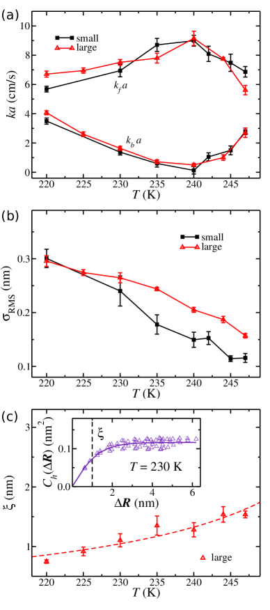
Figure 5: (a) Forward ($k_{f}$) and backward ($k_{b}$) rates representing freezing and melting processes of the solid-interface for the two different sized systems. Results are multiplied by the measured average step size $a=0.23$ nm which roughly equals the spacing between successive ice planes. (b) The root-mean-squared deviation of the discretized roughened ice surface $\sigma_{{\rm RMS}}$. (c) Spatial correlation lengths $\xi$ for the large systems extracted by fitting the height-difference correlation function shown in the inset as an example at $T=230$ K.

The forward rate $k_{f}$ increases by a factor of $\sim 1.3$ from $247-240$ K, and progressively decreases by a factor of $\sim 1.5$ from $240-220$ K. The backward rate shows a stronger nonmonotonic temperature dependence: decreasing by a factor of $\sim 5$ from 247 K to the minimum at $240$ K, and increasing by roughly the same factor upon further cooling to $220$ K. The nonmonotonic behavior in Fig. 5a shows that the difference between forward and backward processes, and consequently the growth rate $R_{{\rm G}}=(k_{f}-k_{b})a$, is greatest at $240$ K and lowest at both $220$ and $247$ K. While low thermodynamic driving force and increased melting propensity can intuitively describe the small difference in $(k_{f}-k_{b})a$ at $247$ K (see also Figs. 4a-b), it is instructive to analyze how changes in interfacial structure coupled with arrested water dynamics Weiss et al. (2011) and increased tetrahedrality of the liquid Moore and Molinero (2011) can limit the attachment kinetics that microscopically underpin the forward and backward rates at low temperatures.

The microscopic features of the interfacial regions are intricately linked to nonmonotonic temperature dependence of the forward and backward processes at increasingly lower temperatures. Notably, the structural characteristics of the solid-liquid interface scale differently than in solid-vapor systems. Fig. 5b shows the root-mean-squared (RMS) deviation of the discretized fibers used to define the instantaneously roughened solid-interface for all temperatures. The figure shows that the dividing surface becomes rougher as the temperature is lowered, consistent with previous simulations, Pirzadeh et al. (2012) but opposite to what is observed at the ice-vapor interface. Cahn and Hilliard (1958); Libbrecht (2005) The RMS deviation is slightly larger than 0.3 nm at the coldest temperatures, corresponding approximately to an extra ice layer, or half a hexagon as viewed from the basal direction. The larger systems show higher RMS deviations at higher temperatures, which is a notable finite-size effect.

Small systems in particular can lead to overestimated growth kinetics. Rozmanov and Kusalik (2011) To understand how this arises, Fig. 5c shows the roughness correlation length $\xi$ extracted from the height-difference spatial correlation function for the large systems, Weeks and Gilmer (1979); Salditt et al. (1995)

$$C_{h}(\Delta{\bf R})=\langle|h({\bf r})-h({\bf r^{\prime}})|^{2}\rangle\,,$$ (5)

where $h({\bf r})$ is the height of the discretized fiber (in this case, its extent along the $x$-direction) at position ${\bf r}$ along the cross-sectional area of the roughened surface, and $\Delta{\bf R}={\bf r}-{\bf r^{\prime}}$. The roughness correlation length was extracted by fitting the function $C_{h}(\Delta{\bf R})$ to the form, Salditt et al. (1995)

$$C_{h}(\Delta{\bf R})=2\sigma^{2}\left\{1-\exp\left[-(\Delta{\bf R}/\xi)^{(2P)}\right]\right\}\,,$$ (6)

where $\sigma$ is the standard deviation in heights, $\xi$ is the correlation length, and $P$ is a roughness exponent, typically between 0.5 and 0.6 for the large systems. The temperature dependence of $\xi$ can be fitted to the Kosterlitz-Thouless scaling relation (dashed line), which increases exponentially and diverges at the roughening transition temperature near the melting point. Kosterlitz and Thouless (1973) At $247$ K, the roughness correlation length is nearly $1.6$ nm, almost half the size of the large system simulation cell. These data indicate that finite size effects will become prevalent if long-wavelength capillary waves driving the roughening transition are damped out due to small simulation cells. Higher observed growth rates in sufficiently small systems could result due to the appearance of defected surface motifs that aid molecular rearrangement near the solid surface. Weeks and Gilmer (1979); Broughton and Gilmer (1983)

The increase in the roughness correlation length with temperature in Fig. 5c shows structural features are more correlated at higher temperatures. Consequently, the solid-interface appears smoother, with a smaller RMS deviation in the height profiles of the discretized fibers. At lower temperatures, structural correlations occur over shorter lengthscales, and the ice surface becomes rougher.

To gain insight into which properties of the roughened interface inhibit molecular retention at low temperatures, we track where incoming molecules contact the intermediate ice layer (IIL), which is typically composed of a few roughened water layers above the ice boundary as described in Appendix A. We divide the flux of these incoming molecules into molecules that freeze, and molecules that escape back to the liquid without being incorporated in the solid phase. We measure the average distance $d$ of a water molecule to this IIL, and additionally, the curvature $\kappa$ of the roughened surface at the contact point. Contact is defined by the formation of hydrogen bonds between the incoming water molecule and molecules that are part of the IIL. The mean curvature $\kappa$ at each point of the atomistically rough intermediate ice surface was calculated from the average of the principal curvatures, $\kappa=\frac{1}{2}(\kappa_{{\rm min}}+\kappa_{{\rm max}})$, where $\kappa_{{\rm min}}$ and $\kappa_{{\rm max}}$ are the eigenvalues of the shape operator representing the minimum and maximum degree of deflection of a surface at a given point. Toponogov (2006)

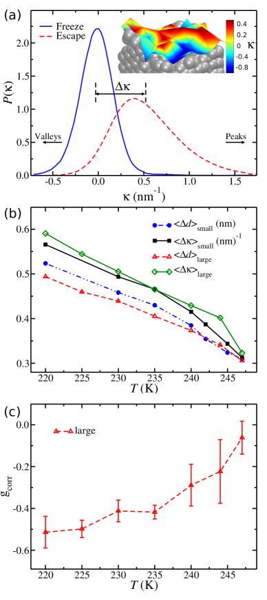
Figure 6: (a) Mean curvature distributions $\kappa$ of freeze, and escape populations at $T=230$ K. The inset shows a colormap of the resulting curvature values atop an instantaneous configuration of the intermediate ice layer. (b) Differences between freeze and escape distributions for the two measures, $\langle\Delta d\rangle$ and $\langle\Delta\kappa\rangle$, for the two system sizes. (c) Statistical correlation $g_{{\rm corr}}$ between low growth rate and high surface roughness for the large systems.

As an example, Fig. 6a shows the curvature distributions for the freezing and escaping populations averaged over all trajectories at $230$ K. Molecules that directly freeze tend to dock in concave valleys, or regions of negative (or near zero) mean curvature on the roughened intermediate ice surface. Conversely, molecules that escape back into the liquid tend to bind to peaks, or regions of high mean curvature farther away from the solid interface. Particles subsequently have a greater propensity to escape from convex surfaces than from concave surfaces of ice, as seems to be the case for liquid-vapor interfaces as well (see Refs.[Weeks and Gilmer, 1979; Willard and Chandler, 2010]).

Fig. 6b measures the degree of overlap between the freeze and escape distributions for both observables, quantified by taking differences in the mean values: $\Delta\kappa=\langle\kappa_{{\rm escape}}\rangle-\langle\kappa_{{\rm freeze}}\rangle$ and $\Delta d=\langle d_{{\rm escape}}\rangle-\langle d_{{\rm freeze}}\rangle$. The differences in both $\Delta\kappa$ and $\Delta d$ decrease as the temperature approaches the melting point, where the solid surface is much flatter. Analogously, there are fewer peaks and valleys for the smoother interfaces at higher temperatures, and less of a docking preference between freeze and escape populations. At large undercoolings, however, the separation between distributions is larger, indicating that escape events preferentially bind to regions of higher curvature. These roughened structural features may develop in order to expose the more stable prismatic face to the liquid contact. Nada and Furukawa (2005); Pereyra and Carignano (2009) Although, surface roughening has been noted to appear on the prismatic and basal faces of ice as well. Seo et al. (2012)

To asses how the roughened structural features of the ice surface impact the growth kinetics, Fig. 6c shows Pearson’s statistical correlation coefficient $g_{{\rm corr}}$ between the instantaneous growth rates $R_{{\rm G}}$ and surface roughness $\sigma_{{\rm RMS}}$ for the large systems. Instantaneous growth rates were obtained from 2.0 ns moving windows centered at each frame of the trajectories. The coefficient is $-1.0$ when growth rates are completely anticorrelated with surface roughness. When $g_{{\rm corr}}$ is 0.0, the two measures are uncorrelated. As can be seen in the figure, $g_{{\rm corr}}$ approaches 0.0 at high temperatures, and $-0.51\pm 0.08$ as the temperature is lowered to 220 K. Consequently, low growth rates are increasingly associated with high surface roughness below the temperature of maximum crystallization.

V Summary and conclusions

Using molecular dynamics simulations, we have identified structural features of the ice-liquid interface along the secondary prismatic direction that affect crystal growth velocities in the supercooled regime. Near the melting point, the freezing rate is limited by surface depletion events, as molecules detach from the ice and migrate back to the liquid. At much lower temperatures, the topology of the roughened intermediate ice layer plays an important limiting role hindering ice growth. The decrease in the interfacial retention probability at low temperatures is due to the appearance of high-curvature structural motifs. Along with the increased tetrahedrality of the liquid, Moore and Molinero (2011) these roughened structural profiles limit the crystal growth velocities at larger undercoolings, as the liquid is unable to adjust to the required surface geometry.

At the temperature of maximum crystallization, the efficiency of converting interfacial water to ice is maximized. The rates between competing attachment and detachment reactions in the interfacial region is greatest at this temperature. Notably, molecular detachment rates leading to surface melting are minimized when the crystallization rate is maximized. The liquid is best able to adjust and fill surface pockets at the temperature of maximum growth.

These insights into the molecular scale rate limiting processes for heterogeneous ice nucleation should prove useful in analyzing how other perturbations, such as the presence of solutes, affect the interfacial region and freezing rates. Such an understanding is vital for unraveling the ice growth inhibition mechanisms of antifreeze proteins in biological systems, and for industrial cryogenics applications.

VI Acknowledgments

The authors would like to thank Valeria Molinero for her insightful comments on an early version of this manuscript. This research was supported by a grant to BJB from the National Science Foundation (NSF-CHE-0910943). We thank CCNI at RPI and the XSEDE resources at TACC for providing computational facilities to support this project.

Appendix A Ice-water selectivity

In order to enhance the selectivity between ice- and liquid-like local configurations using the tetrahedral order parameter in Eqn. 1, the atomic positions of the trajectories were first averaged over 5 ps windows to reduce thermal and librational noise in the oxygen atom positions. This time is shorter than the $\sim 10$ ps characteristic water reorientation time for this water model at 250 K, Stirnemann and Laage (2012) which is a higher than any temperature used here and so is much shorter than the characteristic time in which a molecule can interconvert between ice and water in our trajectories. These averaged positions were then used to evaluate the tetrahedral order parameter using Eqn. 1 for each water molecule.

The order parameter history of each water molecule from the position averaged trajectories was then exponentially time-smoothed using, $\langle S_{\theta}\rangle_{t}=\alpha S_{\theta}(t)+(1-\alpha)\langle S_{\theta}\rangle_{t-1}$, where $S_{\theta}(t)$ is the instantaneous order parameter of a given molecule at time $t$, $\langle S_{\theta}\rangle_{t-1}$ is the smoothed order parameter of the previous (position-averaged) time step $t-1$, and $\alpha$ is the smoothing parameter. We found $\alpha\sim 0.3$ gave adequate separation between bulk ice and liquid distributions at low temperatures. This time-based smoothing was used to inhibit instantaneous tetrahedral configurations from contributing to the analysis, which may spontaneously occur even at high temperatures.

Molecules within the interfacial regions whose order parameter $\langle S_{\theta}\rangle_{t}$ was greater than the ice threshold criteria $S_{{\rm tol}}$, but less than 75% of the liquid value at the given temperature, were labeled as intermediate ice. Moore and Molinero (2011) A molecule retained its ice, liquid, or intermediate ice label for the duration of the 5 ps position-averaging window. These labels were only used for population analysis.

Appendix B Interface identification

In order to identify the (moving) positions of the solid- and liquid-interface dividing surfaces, the order parameter $\langle S_{\theta}\rangle_{t}$ was binned across the simulation cell as shown in Fig. 2a. The resulting distributions were fitted to profile functions of the form $f(x)=A\left[\tanh\left(\frac{x-C}{B}\right)-\tanh\left(\frac{x-D}{E}\right)\right]$, where $\{A,B,C,D,E\}$ were the fit parameters. The roots of the fourth derivative of this function lie close to the positions of the shoulders of the profile and were used here to define the locations of the SI and LI dividing surfaces as shown by the dashed vertical lines in Fig. 2a.

The distributions were accrued over 200 ps time windows. This sampling corresponded to roughly one-tenth the time it took the solid-interface to pass through the next layer of ice in the fastest growing trajectories. The positions of the SI boundaries were aligned with the nearest ice plane at each time step since the lower shoulders of the fitted profile function were not necessarily concomitant with the outermost ice layer. Once the interfacial boundaries were established, molecules could be identified as being in the solid (S), liquid (L), or in one of the two interfacial regions (I₁, I₂) at any given time in the trajectory. To remove rapid recrossing events across the boundaries, a molecule was required to reside a minimum of 200 ps in a region before it counted towards the population statistics. Molecular configurations and surfaces were rendered using MATLAB and the Visual Molecular Dynamics (VMD) package. MATLAB (2005); Humphrey et al. (1996)

References

- Kirkpatrick (1975) R. J. Kirkpatrick, Am. Mineral. 60, 798 (1975).
- Levi and Kotrla (1997) A. C. Levi and M. Kotrla, J. Phys.: Condens. Matter. 9, 299 (1997).
- Petrenko and Whitworth (2002) V. F. Petrenko and R. W. Whitworth, Physics of ice (University Press, Oxford, U. K., 2002).
- Koop et al. (2000) T. Koop, B. Luo, A. Tsias, and T. Peter, Nature 406, 611 (2000).
- Murray et al. (2005) B. J. Murray, D. A. Knopf, and A. K. Bertram, Nature 434, 202 (2005).
- Murphy and Koop (2005) D. M. Murphy and T. Koop, Q. J. R. Meteorol. Soc. 131, 1539 (2005), ISSN 1477-870X.
- Cantrell and Heymsfield (2005) W. Cantrell and A. Heymsfield, Bull. Amer. Meteor. Soc. 86, 795 (2005).
- Mazur (1963) P. Mazur, J. Gen. Physiol. 47, 347 (1963).
- Mazur (1970) P. Mazur, 168, 939 (1970).
- Griffith and Ewart (1995) M. Griffith and K. V. Ewart, Biotech. Adv. 13, 375 (1995).
- Feeney and Yeh (1998) R. E. Feeney and Y. Yeh, Trends Food Sci. Technol. 9, 102 (1998).
- Carvajal-Rondanelli et al. (2011) P. A. Carvajal-Rondanelli, S. H. Marshall, and F. Guzman, J. Sci. Food Agric. 91, 2507 (2011).
- Hassas-Roudsari and Goff (2012) M. Hassas-Roudsari and H. D. Goff, Food Res. Int. 46, 425 (2012).
- Libbrecht (2005) K. G. Libbrecht, Rep. Prog. Phys. 68, 855 (2005).
- Bartels-Rausch et al. (2012) T. Bartels-Rausch, V. Bergeron, J. H. E. Cartwright, R. Escribano, J. L. Finney, H. Grothe, P. J. Gutiérrez, J. Haapala, W. F. Kuhs, J. B. C. Pettersson, et al., Rev. Mod. Phys. 84, 885 (2012).
- Beaglehole and Wilson (1993) D. Beaglehole and P. Wilson, J. Phys. Chem. 97, 11053 (1993).
- Pruppacher (1967) H. R. Pruppacher, J. Chem. Phys. 47, 1807 (1967).
- Langer et al. (1978) J. S. Langer, R. F. Sekerka, and T. Fujioka, J. Crys. Growth 44, 414 (1978).
- Furukawa and Shimada (1993) Y. Furukawa and W. Shimada, J. Crys. Growth 128, 238 (1993).
- Shibkov et al. (2005) A. Shibkov, M. Zheltov, A. Korolev, A. Kazakov, and A. Leonov, J. Crys. Growth 285, 215 (2005).
- Wilson (1900) H. A. Wilson, Phil. Mag. 50, 238 (1900).
- Frenkel (1932) J. Frenkel, Phys. Z. Sowjet Union 1, 498 (1932).
- Kolmogorov (1937) A. N. Kolmogorov, Bull. Acad. Sci. URSS (Cl. Sci. Math. Nat.) 3, 355 (1937).
- Johnsson and Mehl (1940) W. A. Johnsson and R. F. Mehl, Trans. Am. Inst. Min. Metall. Eng. 135, 416 (1940).
- Avrami (1940) M. Avrami, J. Chem. Phys. 8, 212 (1940).
- Karim and Haymet (1987) O. A. Karim and A. D. J. Haymet, Chem. Phys. Lett. 138, 531 (1987).
- Karim O. A. Haymet (1988) A. D. J. Karim O. A. Haymet, J. Chem. Phys. 89, 6889 (1988).
- Nada and Furukawa (1995) H. Nada and Y. Furukawa, Jpn. J. Appl. Phys. 34, 583 (1995).
- Baéz and Clancy (1995) L. A. Baéz and P. Clancy, J. Chem. Phys. 103, 9744 (1995).
- Hayward and Haymet (2001) J. A. Hayward and A. D. J. Haymet, J. Chem. Phys. 114, 3713 (2001).
- Hayward and Haymet (2002) J. A. Hayward and A. D. J. Haymet, Phys. Chem. Chem. Phys. 4, 3712 (2002).
- Nada and Furukawa (2005) H. Nada and Y. Furukawa, J. Crys. Growth 283, 242 (2005).
- Carignano et al. (2005) M. A. Carignano, P. Shepson, and I. Szleifer, Mol. Phys. 103, 2957 (2005).
- Kim and Yethiraj (2008) J. S. Kim and A. Yethiraj, J. Chem. Phys. 129, 124504 (2008).
- Kim et al. (2009) J. S. Kim, S. Damodaran, and A. Yethiraj, J. Phys. Chem. A 113, 4403 (2009).
- Pirzadeh and Kusalik (2010) P. Pirzadeh and P. G. Kusalik, J. Am. Chem. Soc. 133, 704 (2010).
- Rozmanov and Kusalik (2011) D. Rozmanov and P. G. Kusalik, Phys. Chem. Chem. Phys. 13, 15501 (2011).
- Pirzadeh et al. (2012) P. Pirzadeh, E. N. Beaudoin, and P. G. Kusalik, Crys. Growth Des. 12, 124 (2012).
- Seo et al. (2012) M. Seo, E. Jang, K. Kim, S. Choi, and J. S. Kim, J. Chem. Phys. 137, 154503 (2012).
- Rozmanov and Kusalik (2012a) D. Rozmanov and P. G. Kusalik, Phys. Chem. Chem. Phys. 14, 13010 (2012a).
- Rozmanov and Kusalik (2012b) D. Rozmanov and P. G. Kusalik, J. Chem. Phys. 137, 094702 (2012b).
- Moore and Molinero (2011) E. B. Moore and V. Molinero, Nature 479, 506 (2011).
- Shepherd et al. (2012) T. D. Shepherd, M. A. Koc, and V. Molinero, J. Phys. Chem. C 116, 12172 (2012).
- Weiss et al. (2011) V. C. Weiss, M. Rullich, C. Köhler, and T. Frauenheim, J. Chem. Phys. 135, 034701 (2011).
- Rost et al. (2003) M. J. Rost, D. A. Quist, and J. W. M. Frenken, Phys. Rev. Lett. 91, 026101 (2003).
- Abascal and Vega (2005) J. L. F. Abascal and C. Vega, J. Chem. Phys. 123, 234505 (2005).
- Hess et al. (2008) B. Hess, C. Kutzner, D. van der Spoel, and E. Lindahl, J. Chem. Theory Comput. 4, 435 (2008).
- Essmann et al. (1995) U. Essmann, L. Perera, M. L. Berkowitz, T. Darden, H. Lee, and L. G. Pedersen, J. Chem. Phys. 103, 8577 (1995).
- Parrinello and Rahman (1981) M. Parrinello and A. Rahman, J. Appl. Phys. 52, 7182 (1981).
- Stirnemann and Laage (2012) G. Stirnemann and D. Laage, J. Chem. Phys. 137 (2012).
- Fernández et al. (2006) R. G. Fernández, J. L. F. Abascal, and C. Vega, J. Chem. Phys. 124, 144506 (2006).
- Bernal and Fowler (1933) J. D. Bernal and R. H. Fowler, J. Chem. Phys. 1, 515 (1933).
- Chau and Hardwick (1998) P.-L. Chau and A. J. Hardwick, Mol. Phys. 93, 511 (1998).
- Razul and Kusalik (2011) M. S. G. Razul and P. G. Kusalik, J. Phys. Chem. 134, 014710 (2011).
- Bauerecker et al. (2008) S. Bauerecker, P. Ulbig, V. Buch, L. Vrbka, and P. Jungwirth, J. Phys. Chem. C 112, 7631 (2008).
- Mishima and Stanley (1998) O. Mishima and H. E. Stanley, Nature 396, 329 (1998).
- Moore and Molinero (2010) E. B. Moore and V. Molinero, J. Chem. Phys. 132, 244504 (2010).
- Abascal and Vega (2010) J. L. F. Abascal and C. Vega, J. Chem. Phys. 133, 234502 (2010).
- Malaspina et al. (2013) D. C. Malaspina, A. J. B. di Lorenzo, R. G. Pereyra, I. Szleifer, and M. A. Carignano, J. Chem. Phys. 139, 024506 (2013).
- Spitzer (1976) F. Spitzer, Principles of random walk (Springer-Verlag, New York, U. S. A., 1976).
- Jorgensen et al. (1983) W. L. Jorgensen, J. Chandrasekhar, J. D. Madura, R. W. Impey, and M. L. Klein, J. Chem. Phys. 79, 926 (1983).
- Cahn and Hilliard (1958) J. W. Cahn and J. E. Hilliard, J. Chem. Phys. 28, 258 (1958).
- Weeks and Gilmer (1979) J. D. Weeks and G. H. Gilmer, in Advances in chemical physics, edited by I. Prigogine and S. A. Rice (John Wiley, New York, 1979), vol. 40, pp. 157–228.
- Salditt et al. (1995) T. Salditt, T. H. Metzger, C. Brandt, U. Klemradt, and J. Peisl, Phys. Rev. B 51, 5617 (1995).
- Kosterlitz and Thouless (1973) J. M. Kosterlitz and D. J. Thouless, J. Phys. C: Sol. Stat. Phys. 6, 1181 (1973).
- Broughton and Gilmer (1983) J. Q. Broughton and G. H. Gilmer, J. Chem. Phys. 79, 5119 (1983).
-
Toponogov (2006)
V. A. Toponogov,
Differential Geometry of Curves and
Surfaces: A Concise Guide (Birkhäuser, Boston, U. S. A., 2006). - Willard and Chandler (2010) A. P. Willard and D. Chandler, J. Phys. Chem. B 114, 1954 (2010).
- Pereyra and Carignano (2009) R. G. Pereyra and M. A. Carignano, J. Phys. Chem. C 113, 12699 (2009).
- MATLAB (2005) MATLAB, version 7.0.1 (R14SP1) (The MathWorks Inc., Natick, Massachusetts, 2005).
- Humphrey et al. (1996) W. Humphrey, A. Dalke, and K. Schulten, J. Mol. Graph. 14, 33 (1996).