Low regularity well-posedness for the 2D Maxwell-Klein-Gordon equation in the Coulomb gauge

Abstract.

We consider the Maxwell-Klein-Gordon equation in 2D in the Coulomb gauge. We establish local well-posedness for $s=\frac{1}{4}+\epsilon$ for data for the spatial part of the gauge potentials and for $s=\frac{5}{8}+\epsilon$ for the solution $\phi$ of the gauged Klein-Gordon equation. The main tool for handling the wave equations is the product estimate established by D’Ancona, Foschi, and Selberg. Due to low regularity, we are unable to use the conventional approaches to handle the elliptic variable $A_{0}$, so we provide a new approach.

1. Introduction

We study local well-posedness (LWP) of the Cauchy problem for the 2D Maxwell-Klein-Gordon equation (MKG) in the Coulomb gauge. Well-posedness for MKG in 2D has been so far only considered in the Lorenz and temporal gauges. Moncrief [12] showed global well-posedness in the Lorenz gauge for data in $H^{2}$. Recently Pecher [13] studied LWP for data with $s=\frac{1}{4}+\epsilon$ for the gauge potentials and $s=\frac{3}{4}+\epsilon$ for $\phi$, the solution of the gauged Klein-Gordon equation. In the temporal gauge, there is work by Schwarz [14] for $s\geq 2$ and with $\left|\phi\right|\rightarrow 1$ at infinity.

Based on the previous works for wave equations in 2D the common expectation could be that MKG in the Coulomb gauge should be well-posed for $s>\frac{1}{4}$ (we explain this below). Moreover, it might seem that this is obvious and that it should simply follow from well-known estimates. However, at this low level of regularity even solving the elliptic equation comes with obstacles. As a result, low regularity well-posedness for MKG in 2D becomes more interesting than initially expected.

In the Coulomb gauge, MKG is a system of wave equations for the complex field $\phi$ and the spatial part of the connection $A$ coupled to elliptic equations for the temporal parts, $A_{0}$ and $\partial_{t}A_{0}$. The nonlinearities involve null forms and other bilinear and trilinear terms.

The null condition was introduced by Klainerman in [7], and it was first used to lower regularity assumptions on initial data in [5]. The null form in MKG in the Coulomb gauge was originally uncovered in [6].

The null form appearing in MKG is

$$Q_{\alpha\beta}(u,v)=\partial_{\alpha}u\partial_{\beta}v-\partial_{\beta}u\partial_{\alpha}v.$$

In 3D, almost optimal LWP for initial data in $H^{s}\times H^{s-1},s>\frac{3}{2}$, for wave equations with this particular null form was shown in [8]. For example, for systems that can be written as

$$\Box u=Q_{\alpha\beta}(u,v)=\Box v,\quad\alpha,\beta\in\{0,\dots,3\},\ \alpha\neq\beta.$$

In 2D, the situation is not as optimal. Note that by scaling invariance, $s=\frac{n}{2}$ is the critical exponent for the system on $\mathbb{R}^{n+1}$. By examining the first iterate Zhou [18] showed that $s>\frac{5}{4}$ is as close as one can get using iteration methods (but see [3]).

Now, if we do not consider the elliptic equation, cubic terms or bilinear terms involving the elliptic variables, MKG in the Coulomb gauge can be schematically written as

(1.1) $$\begin{split}\Box u&=D^{-1}Q_{\alpha\beta}(u,v),\\ \Box v&=Q_{\alpha\beta}(D^{-1}u,v).\end{split}$$

The presence of $D^{-1}=(-\Delta)^{-\frac{1}{2}}$ changes the scaling transformation and shifts the critical exponent to $\frac{n}{2}-1$.

Machedon and Sterbenz [11] established almost optimal LWP for MKG in 3D for $s>\frac{1}{2}$. In addition, they showed that the system (1.1) will be ill-posed below $\frac{3}{4}$ if one only considers the above model equations.

Now, because of [18] and $D^{-1}$ heuristically one might expect MKG to be locally well-posed for $s>\frac{1}{4}$. However, this same heuristic raises an expectation of (1.1) being well-posed for $s>\frac{1}{2}$ in 3D, but again [11] showed $s>\frac{3}{4}$ is needed.

In this paper we show that $s>\frac{1}{2}$ is needed if we only use the wave analog of $X^{s,b}$ spaces (defined in Section 2.2 below) and assume $A$ and $\phi$ have the same regularity. However, we also show that we can let $s^{\prime}=\frac{1}{4}+\epsilon$ for $A_{j}$ if $s=\frac{5}{8}+\epsilon$ for $\phi$ (see Theorem 1.1 for a precise statement).

We note that one of the observations that allowed [11] to lower the regularity was the recognition of the cancellations between the null form and the elliptic term in the wave equation for $\phi$. Here the need for $s>\frac{1}{2}$ comes already in the equation for $A_{j}$.

The main technical tool for handling the wave equation estimates is the convenient atlas of product estimates established by D’Ancona, Foschi, and Selberg [2] (see Theorem 2.1 below).

Finally, controlling the elliptic estimates for $A_{0}(t)$ in 2D when $s<1$ causes difficulties when one attempts the standard methods. We provide an alternative approach to resolve this.

1.1. MKG system and the statement of the results

MKG is a system of Euler-Lagrange equations of the following action functional

(1.2) $$\mathcal{L}(A,\phi)=\int_{\mathbb{R}^{2+1}}\frac{1}{2}D_{\alpha}\phi D^{\alpha}\phi+\frac{1}{4}F_{\alpha\beta}F^{\alpha\beta}\;\mathrm{d}x\mathrm{d}t.$$

Here

$$\phi:\mathbb{R}^{2+1}\to{\mathbb{C}},\quad A\mbox{ is a $1$-form with components }\quad A_{\alpha}:\mathbb{R}^{2+1}\rightarrow\mathbb{R},\ \ \alpha\in\{0,1,2\},$$

$D_{\alpha}$ denotes the covariant derivative

$$D_{\alpha}\phi:=(\partial_{\alpha}+iA_{\alpha})\phi,$$

and $F:=dA$, so that

$$F_{\alpha\beta}=\partial_{\alpha}A_{\beta}-\partial_{\beta}A_{\alpha},\qquad\alpha,\beta\in\{0,1,2\}.$$

One may regard $A$ as a $U(1)$ connection and $F$ as the associated curvature.

In (1.2) we sum over repeated upper and lower indices, and we raise and lower indices with the Minkowski metric $(\eta^{\alpha\beta})=(\eta_{\alpha\beta})=\mbox{diag}(-1,1,1)$ so that

$$D^{\alpha}\phi=\eta^{\alpha\beta}D_{\beta}\phi,\quad\quad F^{\alpha\beta}=\eta^{\alpha\gamma}\eta^{\beta\delta}F_{\gamma\delta}.$$

The Euler-Lagrange equations associated with the action functional (1.2) are

(1.3a) $$D_{\alpha}D^{\alpha}\phi =0,$$

(1.3b) $$\partial_{\alpha}F^{\alpha\beta} =J^{\beta},\quad\beta\in\{0,1,2\},$$

where $J^{\beta}$ is the current given by

$$J^{\beta}=-\Im(\phi\overline{D^{\beta}\phi}),$$

and $\Im(z)$ denotes the imaginary part of the complex number $z$.

The action functional (1.2) is invariant under the action of the $U(1)$ group, so for any sufficiently regular $f:\mathbb{R}^{2+1}\rightarrow\mathbb{R}$ we have

$$\mathcal{L}(\phi,A)=\mathcal{L}(e^{if}\phi,A-df).$$

In the Coulomb gauge, $\partial^{j}A_{j}=0$, and (1.3a)-(1.3b) become

(1.4a) $$\Delta A_{0} =-\Im(\phi\overline{\partial_{t}\phi})+\left|\phi\right|^{2}A_{0},$$

(1.4b) $$\operatorname{\square}A_{j} =-\Im(\phi\overline{\partial_{j}\phi})+\left|\phi\right|^{2}A_{j}-\partial_{j}\partial_{t}A_{0},$$

(1.4c) $$\operatorname{\square}\phi =-2iA^{j}\partial_{j}\phi+2iA_{0}\partial_{t}\phi+i(\partial_{t}A_{0})\phi+A^{\alpha}A_{\alpha}\phi,$$

(1.4d) $$\partial^{j}A_{j} =0.$$

As is now well-known, the equations (1.4a)-(1.4d) can be rewritten further as a system involving null forms (see [6, 10, 16, 11, 4])

(MKG-0) $$\Delta A_{0} =-\Im(\phi\overline{\partial_{t}\phi})+|\phi|^{2}A_{0}$$

(MKG-1) $$\Delta\partial_{t}A_{0} =-\Im\partial_{j}(\phi\overline{\partial_{j}\phi})+\partial_{j}(|\phi|^{2}A_{j}),$$

(MKG-2) $$\Box A_{j} =2R^{k}D^{-1}Q_{jk}(\Re\phi,\Im\phi)+\mathcal{P}(|\phi|^{2}A_{j}),$$

(MKG-3) $$\Box\phi =-iQ_{jk}{(\phi,D^{-1}[R^{j}A^{k}-R^{k}A^{j}])}+2iA_{0}\partial_{t}\phi+i(\partial_{t}A_{0})\phi+A^{\mu}A_{\mu}\phi,$$

(MKG-4) $$\partial^{j}A_{j} =0,$$

where $R_{k}$ denotes the Riesz transform, $\mathcal{P}$ is the Leray projection onto the divergence free vector fields, $\mathcal{P}=\Delta^{-1}d^{\ast}d$, or equivalently

$$\mathcal{P}X_{j}=R^{k}(R_{j}X_{k}-R_{k}X_{j}),$$

and $Q_{\alpha\beta}$ denotes the null form

$$Q_{\alpha\beta}(u,v)=\partial_{\alpha}u\partial_{\beta}v-\partial_{\beta}v\partial_{\alpha}u.$$

The main result of this paper is contained in the following theorem.

Theorem 1.1.

Let $\frac{1}{4}<s^{\prime}\leq 1,\ \ \frac{1}{2}<s\leq 1,$ and in addition, let $s^{\prime}$ satisfy

(1.5) $$\max\left(\frac{3}{2}-2s,\frac{s}{2}-\frac{1}{8}\right)<s^{\prime}<4s-\frac{3}{2}.$$

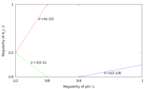
Figure 1.

Consider MKG in the Coulomb gauge given by (MKG-0)-(MKG-4) with initial data

(1.6) $$(A_{1},A_{2},\phi)|_{t=0} =(a_{1},a_{2},\phi_{0})\in H^{s^{\prime}}\times H^{s^{\prime}}\times H^{s},$$

(1.7) $$(\partial_{t}A_{1},\partial_{t}A_{2},\partial_{t}\phi)|_{t=0} =(b_{1},b_{2},\phi_{1})\in H^{s^{\prime}-1}\times H^{s^{\prime}-1}\times H^{s-1},$$

(1.8) $$\partial^{j}a_{j} =\partial^{j}b_{j}=0.$$

Then the Cauchy problem (MKG-0)-(MKG-4), (1.6)-(1.8) is locally well-posed in the following sense:

• (Local Existence) For data given by (1.6)-(1.8) there exist $T>0$ depending continuously on the size of the initial data, and functions

  $$A_{0}\in C_{b}([0,T];\dot{H}^{\sigma^{\prime}}) \cap C^{1}_{b}([0,T];\dot{H}^{\sigma^{\prime}-1}),\ 0<\sigma^{\prime}<1+2s,$$

  $$A_{1},A_{2}\in C_{b}([0,T];H^{s^{\prime}}) \cap C_{b}^{1}([0,T];H^{s^{\prime}-1}),$$

  $$\phi\in C_{b}([0,T];H^{s}) \cap C_{b}^{1}([0,T];H^{s-1}),$$

  which solve (MKG) in the Coulomb gauge on $[0,T]\times\mathbb{R}^{2}$ in the sense of distributions and such that the initial conditions are satisfied.

• (Uniqueness) If $T>0$ and $(A,\phi)$ and $(A^{\prime},\phi^{\prime})$ are two solutions of (MKG) in the Coulomb gauge on $(0,T)\times\mathbb{R}^{2}$ belonging to

  $$(C_{b}([0,T];\dot{H}^{\sigma^{\prime}})\cap C_{b}^{1}([0,T];\dot{H}^{\sigma^{\prime}-1}))\times(\mathcal{H}^{s^{\prime},\theta}_{T})^{2}\times\mathcal{H}^{s,\theta}_{T}$$

  with the same initial data, then $(A,\phi)=(A^{\prime},\phi^{\prime})$ on $(0,T)\times\mathbb{R}^{2}$.

• (Continuous Dependence on the Initial Data) For any $(a_{1},a_{2},\phi_{0})\in(H^{s^{\prime}})^{2}\times H^{s}$ and $(b_{1},b_{2},\phi_{1})\in(H^{s^{\prime}-1})^{2}\times H^{s-1}$ satisfying (1.8) there is a neighborhood $U$ of $(a_{1},a_{2},\phi_{0})\times(b_{1},b_{2},\phi_{1})$ in $(H^{s^{\prime}})^{2}\times H^{s}\times(H^{s^{\prime}-1})^{2}\times H^{s-1}$ such that the solution map

  $$(a_{1},a_{2},\phi_{0})\times(b_{1},b_{2},\phi_{1})\mapsto(A,\phi)$$

  is continuous from $U$ into $(C_{b}([0,T];\dot{H}^{\sigma^{\prime}})\cap C_{b}^{1}([0,T];\dot{H}^{\sigma^{\prime}-1}))\times(C_{b}([0,T];H^{s^{\prime}})\cap C_{b}^{1}([0,T];H^{s^{\prime}-1}))^{2}\times C_{b}([0,T];H^{s})\cap C^{1}_{b}([0,T];H^{s-1})$ .

An immediate corollary (can be also seen from Figure 1) is the following

Corollary 1.2.

Let $\frac{1}{2}<s\leq 1$. Then 2D MKG in the Coulomb gauge is locally well-posed (in the sense stated above) for initial data in $(H^{s})^{3}\times(H^{s-1})^{3}$.

Remark 1.1.

We do not consider $s^{\prime},s>1$ since then the initial data is in $L^{\infty}$ and the estimates are easier.

Remark 1.2.

Figure 1 shows the region, where we can obtain LWP. The region is contained between the three lines and bounded below by $\frac{1}{4}$. The region does not include any of the lines except $s,s^{\prime}=1$. It allows to take $s^{\prime}=\frac{1}{4}+\epsilon$ for $s\in[\frac{5}{8},\frac{3}{4}+\epsilon)$. After that, the values for $s^{\prime}$ are bounded below by one of the lines and require $s^{\prime}>\frac{s}{2}-\frac{1}{8}$.

Remark 1.3.

Spaces $\mathcal{H}^{s,\theta}_{T}$ are defined in Section 2.2.

Remark 1.4.

There is no initial data given for $A_{0},$ because $A_{0}(0)$ can be determined by solving the elliptic equation. We note though that $T$ depends on the data (1.6)-(1.8) and on $A(0)$. See Section 3 for more details.

The outline of the paper is as follows. Section 2 sets notation, introduces spaces, and estimates used. In Section 3 we address the complications that arise in 2D when solving for the elliptic variable $A_{0}$. Section 4 is devoted to the proof of Theorem 1.1, which is reduced to establishing appropriate estimates.

Acknowledgments.

The first author was partially supported by a grant from the Simons Foundation #246255.

2. Preliminaries

First we establish notation, then we introduce function spaces as well as estimates used.

2.1. Notation

We use $a\lesssim b$ to denote $a\leq Cb$ for some positive constant $C$. Also, $a\simeq b$ means $a\lesssim b$ and $b\lesssim a$. A point in the $2+1$ dimensional Minkowski space is written as $(t,x)=(x^{\alpha})_{0\leq\alpha\leq 2}.$ We also use $\underline{U}$ to denote just the spatial part $(U_{1},U_{2})$ of a vector $(U_{0},U_{1},U_{2})$. Greek indices range from $0$ to $2$, and Roman indices range from $1$ to $2$. We raise and lower indices with the Minkowski metric, $\operatorname{diag}(-1,1,1)$. We write $\partial_{\alpha}=\partial_{x^{\alpha}}$ and $\partial_{t}=\partial_{0}$, and we also use the Einstein notation. Therefore, $\partial^{i}\partial_{i}=\triangle,$ and $\partial^{\alpha}\partial_{\alpha}=-\partial^{2}_{t}+\triangle=\square$.

2.2. Function Spaces

Define following Fourier multiplier operators

(2.1) $$\widehat{\Lambda^{\alpha}f}(\xi) =(1+|\xi|^{2})^{\frac{\alpha}{2}}\hat{f}(\xi),$$

(2.2) $$\widehat{\Lambda^{\alpha}_{+}u}(\tau,\xi) =(1+\tau^{2}+|\xi|^{2})^{\frac{\alpha}{2}}\hat{u}(\tau,\xi),$$

(2.3) $$\widehat{\Lambda^{\alpha}_{-}u}(\tau,\xi) =\left(1+\frac{(\tau^{2}-|\xi|^{2})^{2}}{1+\tau^{2}+|\xi|^{2}}\right)^{\frac{\alpha}{2}}\hat{u}(\tau,\xi),$$

where the symbol of $\Lambda^{\alpha}_{-}$ is comparable to $(1+\big{|}|\tau|-|\xi|\big{|})^{\alpha}$. The corresponding homogeneous operators are denoted by $D^{\alpha},D_{+}^{\alpha},D_{-}^{\alpha}$ respectively.

We employ spaces ${H^{s,\theta_{0}}}$ and $\mathcal{H}^{s,\theta}$ with norms given by

$$\|u\|_{H^{s,\theta}} =\|\Lambda^{s}\Lambda^{\theta}_{-}u\|_{L^{2}(\mathbb{R}^{2+1})},$$

$$\|u\|_{\mathcal{H}^{s,\theta}} =\|u\|_{H^{s,\theta}}+\|\partial_{t}u\|_{H^{s-1,\theta}}.$$

An equivalent norm for ${\mathcal{H}^{s,\theta}}$ is $\|u\|_{{\mathcal{H}^{s,\theta}}}=\|\Lambda^{s-1}\Lambda_{+}\Lambda^{\theta}_{-}u\|_{L^{2}(\mathbb{R}^{2+1})}$. If $\theta>\frac{1}{2}$, we have (see for example [15] )

(2.4) $$H^{s,\theta} \hookrightarrow C_{b}(\mathbb{R};H^{s}),$$

(2.5) $${\mathcal{H}^{s,\theta}} \hookrightarrow C_{b}(\mathbb{R};H^{s})\cap C_{b}^{1}(\mathbb{R};H^{s-1}).$$

We denote the restrictions to the time interval $[0,T]$ by

$$H^{s,\theta}_{T}\quad\mbox{and}\quad\mathcal{H}^{s,\theta}_{T},$$

respectively.

2.3. Estimates Used

We use two kinds of product estimates. For Sobolev spaces we have

(2.6) $$\left\|uv\right\|_{H^{-s_{0}}}\lesssim\left\|u\right\|_{H^{s_{1}}}\left\|v\right\|_{H^{s_{2}}},$$

where $s_{0},s_{1},s_{2}$ satisfy $s_{0}+s_{1}+s_{2}\geq 1,$ and $s_{0}+s_{1}+s_{2}\geq\max(s_{0},s_{1},s_{2})$ and at most one of these inequalities is an equality (see for instance [2]). The ${H^{s,\theta_{0}}}$ analog is the following theorem.

Theorem 2.1.

[2] Let $s_{0},s_{1},s_{2},b_{0},b_{1},b_{2}\in\mathbb{R}$, then the following estimate holds for all $u,v\in\mathcal{S}(\mathbb{R}^{2+1})$

$$\|uv\|_{H^{-s_{0},-b_{0}}}\lesssim\|u\|_{H^{s_{1},b_{1}}}\|v\|_{H^{s_{2},b_{2}}}$$

provided that the following conditions are satisfied:

(2.7a) $$b_{0}+b_{1}+b_{2} >\frac{1}{2}$$

(2.7b) $$b_{0}+b_{1} \geq 0$$

(2.7c) $$b_{0}+b_{2} \geq 0$$

(2.7d) $$b_{1}+b_{2} \geq 0$$

(2.7e) $$s_{0}+s_{1}+s_{2} >\frac{3}{2}-(b_{0}+b_{1}+b_{2})$$

(2.7f) $$s_{0}+s_{1}+s_{2} >1-\min(b_{0}+b_{1},b_{0}+b_{2},b_{1}+b_{2})$$

(2.7g) $$s_{0}+s_{1}+s_{2} >\frac{1}{2}-\min(b_{0},b_{1},b_{2})$$

(2.7h) $$s_{0}+s_{1}+s_{2} >\frac{3}{4}$$

(2.7i) $$(s_{0}+b_{0})+2s_{1}+2s_{2} >1$$

(2.7j) $$2s_{0}+(s_{1}+b_{1})+2s_{2} >1$$

(2.7k) $$2s_{0}+2s_{1}+(s_{2}+b_{2}) >1$$

(2.7l) $$s_{1}+s_{2} \geq\max(0,-b_{0})$$

(2.7m) $$s_{0}+s_{2} \geq\max(0,-b_{1})$$

(2.7n) $$s_{0}+s_{1} \geq\max(0,-b_{2})$$

3. Elliptic variables $A_{0}$ and $\partial_{t}A_{0}$

In this section we address the existence, uniqueness and regularity of the elliptic variable $A_{0}$ and its time derivative.

3.1. Solving for $A_{0}$

We discuss three conventional approaches that we were not able to apply to produce estimates on $A_{0}$.

First, from variational methods, for each $t$ we could obtain existence and uniqueness of $A_{0}(t)$ in $H^{1}(\mathbb{R}^{2})$ as the minimizer of

$$\int_{\mathbb{R}^{2}}\left|\nabla A_{0}\right|^{2}+\left|D_{0}\phi\right|^{2}\mathrm{d}x.$$

Then $A_{0}(t)$ would solve

(3.1) $$\Delta A_{0}=-\Im(\phi\overline{D_{0}\phi})$$

as needed. However, the complications arise when we would like to arrange $A_{0}(t)$ into a solution in some space-time norm. The complications come from the fact that the variational methods do not give us estimates for the $H^{1}$ norm, and for example, the clever manipulations used in [4] to obtain bounds on the homogeneous $\dot{H}^{1}$ norm only seem to work in 3D or higher (or at a higher regularity in 2D: $s\geq 1$). Moreover, even in $3D$ the authors were not able to obtain estimates to bound the $L^{2}$ norm of $A_{0}$ and had to isolate low frequencies.

Another choice is to resort to the fixed point method, just like in [1], and solve the elliptic equation $\eqref{eA0}$ for $A_{0}$, but in 2D, $\log$ is the fundamental solution of the Laplacian, and so far we have not been able to close the iteration in any Sobolev space. In [1], although the elliptic equation was in 2D, it was essentially using the derivative of the fundamental solution of the Laplacian. Hence, it was more tractable.

We could also try to use the Riesz Representation Theorem (in $H^{1}$), but then again this would not give us uniform estimates for $A_{0}(t)$ unless we have $s\geq 1$ (compare with 4D in [16]). (We allow $s=1$ in this paper, but again we are really interested in $s<1$, so we seek a method that works below $1$.) We note however, that we could get an estimate on $\dot{H}^{1}$, but in 2D this is not useful unless we include BMO in the estimates.

Fortunately, there is another choice. The equation for $\partial_{t}A_{0}$ is better behaved than (3.1), and we can solve for $B_{0}=\partial_{t}A_{0}$ in $C_{b}([0,T];\dot{H}^{\sigma})$ (see Section 3.2 below). Then we can let

(3.2) $$A_{0}(t)=\int^{t}_{0}B_{0}(s)\mathrm{d}s+a_{0},$$

where $a_{0}\in H^{1}$ is the solution of the variational problem at $t=0$. Since $\dot{H}^{\sigma}\subset\mathcal{S}^{\prime}$, (3.2) defines a tempered distribution. We need to show that (3.2) solves the required equation, and that $A_{0}$ has enough regularity. In particular, we need $A_{0}\in L^{\infty}$ to handle the estimates for $\phi$ (see Section 4.1.4), so we will use the equation and bootstrap from the initial $\dot{H}^{\sigma}$ estimate (see estimate (3.14), Lemma 3.4 and Corollary 3.5).

Remark 3.1.

Alternatively, we could argue that we have the existence of the solution in $H^{1}$ from the variational method or the Riesz Representation Theorem. Then to obtain estimates on $A_{0}$, we could show that $B_{0}$ is the weak time derivative of $A_{0}$, then use it to show that (3.2) holds, and then still proceed with (3.14), Lemma 3.4 and Corollary 3.5.

In [11, 16] the authors show that if $A_{0}$ solves (3.1) and $B_{0}$ solves (MKG-1), then in fact, $B_{0}=\partial_{t}A_{0}$. Here, by definition $\partial_{t}A_{0}=B_{0}$, but it is not immediately obvious that if $A_{0}$ is defined by (3.2), then $A_{0}$ solves (3.1). However, we can show

Lemma 3.1.

Let $B_{0}$ solve (MKG-1). Then $A_{0}(t)$ given by (3.2) solves (3.1) in a sense of tempered distributions for every $t\in[0,T]$.

Proof.

Recall, the current $J=(J_{0},\underline{J})$ is given by

$$J_{\alpha}(t)=-\Im(\phi(t)\overline{D_{\alpha}\phi(t)}),\quad\alpha=0,1,2.$$

Then (MKG-1) says

$$\Delta B_{0}=\operatorname{div}\underline{J},$$

and we need

$$\Delta A_{0}(t)=J_{0}(t).$$

Note, it is enough to show the current is conserved, i.e.,

(3.3) $$\operatorname{div}\underline{J}=\partial_{t}J_{0},$$

because then from (3.2) we have

$$\Delta A_{0}(t) =\int^{t}_{0}\Delta B_{0}(s)\mathrm{d}s+\Delta a_{0}$$

$$=\int^{t}_{0}\operatorname{div}\underline{J}(s)\mathrm{d}s-\Im(\phi(\overline{\partial_{t}\phi+ia_{0}\phi}))$$

$$=\int^{t}_{0}\partial_{t}J_{0}(s)\mathrm{d}s+J_{0}(0)$$

$$=J_{0}(t),$$

as needed. So we show (3.3). To that end, using similar computations as in [11, 16], compute

(3.4) $$\partial_{t}J_{0}=-\Im(\phi\overline{\partial_{t}^{2}\phi})+(\partial_{t}\left|\phi\right|^{2})A_{0}+\left|\phi\right|^{2}B_{0}.$$

Then by using (1.4c) for $\partial^{2}_{t}\phi$, we have

$$\Im(\phi\overline{\partial_{t}^{2}\phi}) =\Im(\phi\overline{2iA^{j}\partial_{j}\phi})-\Im(\phi\overline{2iA_{0}\partial_{t}\phi})-\Im(\phi\overline{iB_{0}\phi})+\Im(\phi\overline{\Delta\phi})$$

$$=-\operatorname{div}\underline{J}-\Im(\phi\overline{2iA_{0}\partial_{t}\phi})-\Im(\phi\overline{iB_{0}\phi})$$

$$=-\operatorname{div}\underline{J}+(\partial_{t}\left|\phi\right|^{2})A_{0}+\left|\phi\right|^{2}B_{0},$$

where to go from the first to the second line, we combined the first and last term using a product rule and the Coulomb condition. Inserting this into (3.4) gives (3.3). ∎

Next we address uniqueness of the solution of (MKG-0).

Lemma 3.2.

Let $A_{0}(t)$ be the solution of (MKG-0). Then $A_{0}(t)$ is unique in $\dot{H}^{\frac{1}{2}}\cap\dot{H}^{1}$.

Proof.

Let $u,v$ both solve (MKG-0). Then $w=u-v$ solves

$$-\Delta w+\left|\phi\right|^{2}w=0.$$

in a sense of tempered distributions. Because $\mathcal{S}$ is dense in $\dot{H}^{\frac{1}{2}}\cap\dot{H}^{1}$ this implies

$$\int_{\mathbb{R}^{2}}(\left|\nabla w\right|^{2}+\left|\phi\right|^{2}w^{2})\;\mathrm{d}x=0.$$

so $w=0$ a.e. in $\mathbb{R}^{2}$. ∎

Remark 3.2.

$\dot{H}^{\frac{1}{2}}$ here is only convenient and not necessary. We show below that $A_{0}$ has actually better regularity than just $\dot{H}^{\frac{1}{2}}\cap\dot{H}^{1}$.

3.2. Solving for $B_{0}$

Recall (MKG-1)

$$\Delta\partial_{t}A_{0}=-{\partial}_{j}\Im(\phi\overline{\partial_{j}\phi})+{\partial}_{j}(|\phi|^{2}A_{j}).$$

So we let

(3.5) $$B_{0}=\frac{\partial_{j}}{\Delta}J_{j}=-2\pi\frac{x_{j}}{\left|x\right|^{2}}\ast\left(\Im(\phi\overline{\partial_{j}\phi})+\left|\phi\right|^{2}A_{j}\right),$$

and then again, define $A_{0}$ by (3.2). Then (MKG-1) is satisfied.

3.3. Estimates for $A_{0}$ and $\partial_{t}A_{0}$

We start with

Lemma 3.3.

Let $B_{0}(t)$ be given by (3.5). Then $B_{0}$ is the unique solution of (MKG-1) in $C_{b}([0,T];\dot{H}^{\sigma})$, for any $\sigma\in(0,2s-1)$, and

(3.6) $$\left\|B_{0}\right\|_{C_{b}([0,T];\dot{H}^{\sigma})}\lesssim\left\|\phi\right\|_{C_{b}([0,T];H^{s})}^{2}(1+\left\|\underline{A}\right\|_{C_{b}([0,T];H^{s^{\prime}})}).$$

Proof.

First note that by definition and continuity of the right hand side in $\eqref{B0def}$, $B_{0}$ solves (MKG-1) and is continuous in time. Uniqueness will follow from (3.6).

Now, fix $t\in[0,T]$. Using (MKG-1) (or (3.5)), we would like to show

(3.7) $$\|\phi(t)\overline{{\partial}_{j}\phi(t)}\|_{\dot{H}^{\sigma-1}} \lesssim\left\|\phi(t)\right\|_{H^{s}}\left\|\partial_{j}\phi(t)\right\|_{H^{s-1}},$$

(3.8) $$\|\left|\phi(t)\right|^{2}A_{j}(t)\|_{\dot{H}^{\sigma-1}} \lesssim\|\phi(t)\|^{2}_{H^{s}}\|A_{j}(t)\|_{H^{s^{\prime}}}.$$

For (3.7), we use duality and show

(3.9) $$\|uv\|_{H^{1-s}}\lesssim\|u\|_{H^{s}}\|v\|_{\dot{H}^{1-\sigma}}.$$

First

$$\begin{split}\|uv\|_{H^{1-s}}&\lesssim\|uv\|_{L^{2}}+\|D^{1-s}(uv)\|_{L^{2}}\\ &\lesssim\|uv\|_{L^{2}}+\|(D^{1-s}u)v\|_{L^{2}}+\|uD^{1-s}v\|_{L^{2}}\\ &=I+II+III.\end{split}$$

By Hölder’s with $\frac{1}{2}={\frac{1-\sigma}{2}}+(\frac{1}{2}-{\frac{1-\sigma}{2}})$ we have

$$I\lesssim\|u\|_{(\frac{1}{2}-\frac{\sigma}{2})^{-1}}\|v\|_{(\frac{1}{2}-{\frac{1-\sigma}{2}})^{-1}}\lesssim\|u\|_{\dot{H}^{\sigma}}\left\|v\right\|_{\dot{H}^{1-\sigma}}\lesssim\|u\|_{H^{s}}\left\|v\right\|_{\dot{H}^{1-\sigma}},$$

as long as

(3.10) $$\sigma\leq s\quad\mbox{ and}\quad 0<\sigma<1.$$

Next, by the same application of Hölder’s

$$II\lesssim\|D^{1-s}u\|_{(\frac{1}{2}-\frac{\sigma}{2})^{-1}}\|v\|_{(\frac{1}{2}-{\frac{1-\sigma}{2}})^{-1}}\lesssim\|D^{1-s}u\|_{\dot{H}^{\sigma}}\left\|v\right\|_{\dot{H}^{1-\sigma}}\lesssim\|u\|_{H^{s}}\left\|v\right\|_{\dot{H}^{1-\sigma}},$$

provided

(3.11) $$\sigma\leq 2s-1\quad\mbox{ and}\quad 0<\sigma<1.$$

Similarly, by Hölder’s with $\frac{1}{2}=\frac{s-\sigma}{2}+(\frac{1}{2}-\frac{s-\sigma}{2})=\frac{1}{2}-\frac{1-s+\sigma}{2}+(\frac{1}{2}-\frac{s-\sigma}{2})$

$$III \lesssim\|u\|_{(\frac{1}{2}-\frac{1-s+\sigma}{2})^{-1}}\|D^{1-s}v\|_{(\frac{1}{2}-\frac{s-\sigma}{2})^{-1}}$$

$$\lesssim\|u\|_{\dot{H}^{1-s+\sigma}}\|D^{1-s+s-\sigma}v\|_{2}$$

$$\lesssim\|u\|_{H^{s}}\|v\|_{\dot{H}^{1-\sigma}}$$

if

(3.12) $$\sigma\leq 2s-1\quad\mbox{ and}\quad 0<\sigma<s.$$

This completes the proof of (3.7). Now for (3.8), we would like to show

$$\|uvw\|_{\dot{H}^{\sigma-1}}\lesssim\|u\|_{H^{s}}\|v\|_{H^{s}}\|w\|_{H^{s^{\prime}}}.$$

By Sobolev embedding and Hölder’s we have

$$\|uvw\|_{\dot{H}^{\sigma-1}} \lesssim\|uvw\|_{\frac{2}{2-\sigma}}$$

$$\lesssim\|uv\|_{{\frac{2}{1-\sigma}}}\|w\|_{2}$$

$$\lesssim\|uv\|_{H^{\sigma}}\|w\|_{H^{s^{\prime}}}$$

$$\lesssim\|u\|_{H^{s}}\|v\|_{H^{s}}\|w\|_{H^{s^{\prime}}},$$

where to go to the last line we use (2.6) provided

(3.13) $$\sigma\leq 2s-1\quad\mbox{ and}\quad\sigma<s.$$

Collecting (3.10)-(3.13) and using $s\leq 1$, we obtain $\sigma\in(0,2s-1).$

∎

Next, from (3.2) and (3.6), we immediately get $A_{0}\in C_{b}([0,T];\dot{H}^{\sigma})$ and

(3.14) $$\left\|A_{0}\right\|_{C_{b}([0,T];\dot{H}^{\sigma})} \lesssim T\left\|\phi\right\|_{C_{b}([0,T];H^{s})}^{2}(1+\left\|\underline{A}\right\|_{C_{b}([0,T];H^{s^{\prime}})})+\left\|a_{0}\right\|_{\dot{H}^{\sigma}},$$

where $0<\sigma<2s-1$. Note, from the variational method we have $a_{0}\in H^{1}$, so $\left\|a_{0}\right\|_{\dot{H}^{\sigma}}$ is finite; we just do not have the estimates to control it in terms of the data for $\phi$ and $\underline{A}$. Also, because $\left\|a_{0}\right\|_{\dot{H}^{\sigma}}$ appears in (3.14), it will appear in (4.4) and (4.7), and hence $T$ will also depend on $\left\|a_{0}\right\|_{\dot{H}^{\sigma}}$.

Lemma 3.4.

Let $\frac{1}{2}<s\leq 1$, and $A_{0}\in C_{b}([0,T];\dot{H}^{\sigma}),\ 0<\sigma<2s-1$. Then $A_{0}\in C_{b}([0,T];\dot{H}^{a})$, where $1<a<2s$, and

$$\left\|A_{0}\right\|_{C_{b}([0,T];\dot{H}^{a})}\lesssim\left\|\phi\right\|_{C_{b}([0,T];H^{s})}\left\|\phi_{t}\right\|_{C_{b}([0,T];H^{s-1})}+\left\|\phi\right\|_{C_{b}([0,T];H^{s})}^{2}\left\|A_{0}\right\|_{C_{b}([0,T];\dot{H}^{\sigma})},$$

where $0<\sigma<2s-1$.

Proof.

We have

$$\left\|D^{a}A_{0}(t)\right\|_{2}=\left\|D^{a-2}\Delta A_{0}(t)\right\|_{2}=\left\|D^{a-2}J_{0}\right\|_{2}.$$

So we need to estimate $\left\|\phi\phi_{t}\right\|_{\dot{H}^{a-2}}$ and $\left\|A_{0}\left|\phi\right|^{2}\right\|_{\dot{H}^{a-2}}$. For the first estimate we need

$$H^{s}\cdot H^{s-1}\hookrightarrow\dot{H}^{a-2},$$

which is equivalent by duality to

$$\left\|uv\right\|_{H^{1-s}}\lesssim\left\|u\right\|_{H^{s}}\left\|v\right\|_{\dot{H}^{2-a}},$$

but from the assumptions on $a$ and $\sigma$, this is exactly the estimate (3.9).

So we bound the cubic term. Using Sobolev with $\frac{1}{2}=\frac{1}{p}-\frac{2-a}{2}$

$$\left\|A_{0}\left|\phi\right|^{2}\right\|_{\dot{H}^{a-2}}\lesssim\left\|A_{0}\left|\phi\right|^{2}\right\|_{p}.$$

We will be done by Hölder and Sobolev, if we can write $\frac{1}{p}=(\frac{1}{2}-\frac{\sigma}{2})+2(\frac{1}{2}-\frac{\alpha}{2})$ for some $0<\alpha\leq s$, and where $\sigma$ is the number of the derivatives we have on $A_{0}$ using (3.14). But

$$\frac{1}{p}=\frac{1}{2}+\frac{2-a}{2}=\left(\frac{1}{2}-\frac{\sigma}{2}\right)+\frac{2-a+\sigma}{2}=\left(\frac{1}{2}-\frac{\sigma}{2}\right)+2\left(\frac{1}{2}-\frac{\tfrac{a}{2}-\tfrac{\sigma}{2}}{2}\right),$$

and $\frac{a}{2}-\frac{\sigma}{2}\leq s$ as needed. ∎

By interpolation using (3.14) and Lemma 3.4 we have

Corollary 3.5.

$A_{0}\in C_{b}([0,T];\dot{H}^{a}),\ 0<a<2s$.

Remark 3.3.

We note the difference in one derivative on the estimates for $A_{0}$ and $B_{0}$. Since $B_{0}$ is the time derivative of $A_{0}$, this difference on the spatial estimates is quite natural.

4. Proof of Theorem 1.1

As is now well-known (see for example [15, 17]), to show Theorem 1.1 it is enough to estimate the nonlinearities in the appropriate spaces.

4.1. Estimates needed

The estimates for the elliptic equations are discussed in Section 3. For the wave equations we need to estimate

$$\left\|\Lambda^{-1}_{+}\Lambda^{-1+\epsilon}_{-}\mathcal{\Box}A_{j}^{(m)}\right\|_{{\mathcal{H}^{s^{\prime},\theta_{1}}}} =\left\|\Box A_{j}^{(m)}\right\|_{H^{s^{\prime}-1,\theta_{1}-1+\epsilon}}$$

and

$$\|\Lambda^{-1}_{+}\Lambda^{-1+\epsilon}_{-}\mathcal{\Box}\phi^{(m)}\|_{{H^{s,\theta_{0}}}} =\left\|\Box\phi^{(m)}\right\|_{H^{s-1,\theta_{0}-1+\epsilon}}.$$

Since the Riesz transforms are clearly bounded on $L^{2}$, and the Leray projection $\mathcal{P}$ is defined in terms of Riesz transforms, we ignore them in the estimates needed. So it is enough to prove the following

(4.1) $$\|D^{-1}Q_{jk}(\Re\phi,\Im\phi)\|_{H^{s^{\prime}-1,\theta_{1}-1+\epsilon}} \lesssim\|\phi\|_{H^{s,\theta_{0}}}^{2},$$

(4.2) $$\||\phi|^{2}A_{j}\|_{H^{s^{\prime}-1,\theta_{1}-1+\epsilon}} \lesssim\|\phi\|_{H^{s,\theta_{0}}}^{2}\|A_{j}\|_{H^{s^{\prime},\theta_{1}}},$$

(4.3) $$\|Q_{jk}{(\phi,D^{-1}A_{j})}\|_{H^{s-1,\theta_{0}-1+\epsilon}} \lesssim\|\phi\|_{H^{s,\theta_{0}}}\|A_{j}\|_{H^{s^{\prime},\theta_{1}}},$$

(4.4) $$\|A_{0}\partial_{t}\phi\|_{H^{s-1,\theta_{0}-1+\epsilon}} \lesssim\|A_{0}\|_{X_{0}}\|\partial_{t}\phi\|_{H^{s-1,\theta_{0}}},$$

(4.5) $$\|\partial_{t}A_{0}\phi\|_{H^{s-1,\theta_{0}-1+\epsilon}} \lesssim\|\partial_{t}A_{0}\|_{C_{b}([0,T];\dot{H}^{\sigma})}\|\phi\|_{H^{s,\theta_{0}}},\ 0<\sigma<2s-1,$$

(4.6) $$\|A^{2}_{j}\phi\|_{H^{s-1,\theta_{0}-1+\epsilon}} \lesssim\|\phi\|_{H^{s,\theta_{0}}}\|A_{j}\|_{H^{s^{\prime},\theta_{1}}}^{2},$$

(4.7) $$\|A^{2}_{0}\phi\|_{H^{s-1,\theta_{0}-1+\epsilon}} \lesssim\|\phi\|_{H^{s,\theta_{0}}}\|A_{0}\|_{X_{0}}^{2},$$

where we let

$$X_{0} =C_{b}([0,T];L^{\infty}\cap\dot{H}^{a}),\ 1<a<2s.$$

Given $(s,s^{\prime})$ such that

(4.8) $$\frac{1}{4}<s^{\prime}\leq 1,\quad\frac{1}{2}<s\leq 1,$$

and in addition

(4.9) $$\max\left(\frac{3}{2}-2s,\frac{s}{2}-\frac{1}{8}\right)<s^{\prime}<4s-\frac{3}{2},$$

choose $\theta_{0},\theta_{1}$ such that

(4.10) $$\frac{1}{2}< \theta_{0}<\frac{3}{4},$$

(4.11) $$\max\left(\frac{1}{2},1-s^{\prime}\right)< \theta_{1}<\min\left(\frac{3}{4},4s-s^{\prime}-1,2s-\frac{1}{2}\right).$$

The restrictions on $(s,s^{\prime})$ allow us to find $\theta_{1}$ satisfying the required conditions. For convenience of the reader, we add that at some point it is needed that $s^{\prime}<2s-\frac{1}{4}$, but that is guaranteed by the current upper bound on $s^{\prime}$.

4.1.1. Null Forms–Proof of Estimate (4.1)

(4.1) will follow from

(4.12) $$\|D^{-1}Q_{jk}(u,v)\|_{H^{s^{\prime}-1,\theta_{1}-1+\epsilon}}\lesssim\|u\|_{H^{s,\theta_{0}}}\|v\|_{H^{s,\theta_{0}}}.$$

Start by recalling [8]

(4.13) $$Q_{jk}(u,v)\precsim D^{\frac{1}{2}}{D_{-}}^{\frac{1}{2}}(D^{\frac{1}{2}}uD^{\frac{1}{2}}v)+D^{\frac{1}{2}}({D_{-}}^{\frac{1}{2}}D^{\frac{1}{2}}uD^{\frac{1}{2}}v)+D^{\frac{1}{2}}(D^{\frac{1}{2}}u{D_{-}}^{\frac{1}{2}}D^{\frac{1}{2}}v),$$

where $w_{1}\precsim w_{2}$ means $|\hat{w}_{1}|\leq C\hat{w}_{2}$ for some $C>0$.

Next, following [9], we estimate $D^{-1}$ by

(4.14) $$D^{-1}\precsim\Lambda^{-1}|_{\{\left|\xi\right|\geq 1\}}+\Lambda^{-M}D^{-1}|_{\{\left|\xi\right|<1\}},$$

where $M>0$ can be taken as large as we wish. Then for high frequencies using (4.13) since $u$ and $v$ have the same regularity, (4.12) follows from showing

(4.15) $$\|uv\|_{H^{s^{\prime}-\frac{3}{2},\theta_{1}-\frac{1}{2}+\epsilon}} \lesssim\|u\|_{H^{s-\frac{1}{2},\theta_{0}}}\|v\|_{H^{s-\frac{1}{2},\theta_{0}}},$$

(4.16) $$\|uv\|_{H^{s^{\prime}-\frac{3}{2},\theta_{1}-1+\epsilon}} \lesssim\|u\|_{H^{s-\frac{1}{2},\theta_{0}-\frac{1}{2}}}\|v\|_{H^{s-\frac{1}{2},\theta_{0}}}.$$

Then given (4.8)-(4.11) the estimates hold by Theorem 2.1.

Now for low frequencies instead of (4.13) we can use a simpler estimate [9, p. 272]

$$Q_{ij}(u,v)\precsim D(D^{\frac{1}{2}}uD^{\frac{1}{2}}v).$$

This reduces (4.12) to

(4.17) $$\|uv\|_{H^{-M,\theta_{1}-1+\epsilon}}\leq\left\|uv\right\|_{H^{-M,0}}\lesssim\|u\|_{L^{2}_{t}H^{s-\frac{1}{2}}}\|v\|_{L^{\infty}_{t}H^{s-\frac{1}{2}}}\lesssim\|u\|_{H^{s-\frac{1}{2},\theta_{0}}}\|v\|_{H^{s-\frac{1}{2},\theta_{0}}},$$

where the first inequality holds because $\theta_{1}-1+\epsilon\leq 0$ and the third one follows from (2.4) and the trivial embedding $\left\|u\right\|_{H^{0,0}}\lesssim\left\|u\right\|_{H^{0,\alpha}}$ for any $\alpha\geq 0$. Finally, the second inequality follows from a spatial estimate

$$\left\|uv\right\|_{H^{-M}}\lesssim\left\|u\right\|_{H^{s-\frac{1}{2}}}\left\|v\right\|_{H^{s-\frac{1}{2}}}.$$

which in turn holds by (2.6) if $M$ is large enough and $s>\frac{1}{2}$.

4.1.2. Cubic term: Proof of Estimate (4.2)

Again for convenience we record the estimate which implies (4.2)

(4.18) $$\|uvw\|_{H^{s^{\prime}-1,\theta_{1}-1+\epsilon}}\lesssim\|u\|_{H^{s^{\prime},\theta_{1}}}\|v\|_{H^{s,\theta_{0}}}\|w\|_{H^{s,\theta_{0}}}.$$

The estimate follows easily from two applications of (2.6) since $s>\frac{1}{2}$ ($0<\delta<<1$ in the third term appears to cover the case $s^{\prime}=1$)

(4.19) $$\begin{split}\|uvw\|_{H^{s^{\prime}-1,\theta_{1}-1+\epsilon}}\leq\|uvw\|_{H^{s^{\prime}-1,0}}&\lesssim\left\|u\right\|_{L^{2}_{t}H^{s^{\prime}}}\left\|uv\right\|_{L^{\infty}_{t}H^{\delta}}\\ &\lesssim\left\|u\right\|_{H^{s^{\prime},\theta_{1}}}\left\|w\right\|_{H^{s,\theta_{0}}}\left\|v\right\|_{H^{s,\theta_{0}}}.\end{split}$$

(Note this holds for any choice of $\frac{1}{2}<\theta_{0},\theta_{1}<1$.)

Remark 4.1.

In fact, if we use Theorem 2.1 we can have both $s$ and $s^{\prime}$ close to $\frac{1}{4}$. We show this below when we establish (4.6), which is the estimate (4.18) with the roles of $s,\theta_{0}$ and $s^{\prime},\theta_{1}$ reversed.

4.1.3. Null Forms–Proof of Estimate (4.3)

We show

(4.20) $$\|Q_{jk}{(u,D^{-1}v)}\|_{H^{s-1,\theta_{0}-1+\epsilon}}\lesssim\|u\|_{H^{s,\theta_{0}}}\|v\|_{H^{s^{\prime},\theta_{1}}}$$

We use (4.14) again. For high frequencies, (4.13) reduces (4.20) to proving that the following three estimates hold

(4.21) $$\|uv\|_{H^{s-\frac{1}{2},\theta_{0}-\frac{1}{2}+\epsilon}} \lesssim\|u\|_{H^{s-\frac{1}{2},\theta_{0}}}\|v\|_{H^{s^{\prime}+\frac{1}{2},\theta_{1}}},$$

(4.22) $$\|uv\|_{H^{s-\frac{1}{2},\theta_{0}-1+\epsilon}} \lesssim\|u\|_{H^{s-\frac{1}{2},\theta_{0}-\frac{1}{2}}}\|v\|_{H^{s^{\prime}+\frac{1}{2},\theta_{1}}},$$

(4.23) $$\|uv\|_{H^{s-\frac{1}{2},\theta_{0}-1+\epsilon}} \lesssim\|u\|_{H^{s-\frac{1}{2},\theta_{0}}}\|v\|_{H^{s^{\prime}+\frac{1}{2},\theta_{1}-\frac{1}{2}}}.$$

Then in view (4.8)-(4.11), the estimates hold by Theorem 2.1.

For low frequencies instead of (4.13) we use [9, p. 272]

$$Q_{ij}(u,v)\precsim D^{\frac{1}{2}}(D^{\frac{1}{2}}uDv),$$

and reduce (4.20), just like in (4.17), to showing

$$\left\|uv\right\|_{H^{s-\frac{1}{2}}}\lesssim\left\|u\right\|_{H^{s-\frac{1}{2}}}\left\|v\right\|_{H^{M}},$$

which holds by (2.6) if $M$ is large enough.

4.1.4. Elliptic Piece: Proof of Estimate (4.4)

Recall we wish to show

(4.24) $$\|A_{0}\partial_{t}\phi\|_{H^{s-1,\theta-1+\epsilon}}\lesssim\left\|A_{0}\right\|_{X_{0}}\|\partial_{t}\phi\|_{H^{s-1,\theta_{0}}},$$

where

$$X_{0}=C_{b}([0,T];L^{\infty}\cap\dot{H}^{a}),\ 1<a<2s.$$

If we could estimate $A_{0}\in H^{\sigma,0}$ (just like for example authors did in [4]), the left hand side of (4.24) could be bounded using Theorem 2.1 as long as $\sigma>0$. In 2D we have to work a little harder.

Using $\theta-1+\epsilon<0$ first reduce (4.24) to

(4.25) $$\|\langle{D}\rangle^{s-1}(A_{0}\partial_{t}\phi)\|_{L^{2}(\mathbb{R}^{2+1})}\lesssim\left\|A_{0}\right\|_{X_{0}}\|\partial_{t}\phi\|_{H^{s-1,\theta_{0}}},$$

which by Hölder in time can follow from

(4.26) $$\|\langle{D}\rangle^{s-1}(uv)\|_{2}\lesssim\left\|u\right\|_{X_{0,x}}\|v\|_{H^{s-1}},$$

where we denote

$$X_{0,x}=L^{\infty}\cap\dot{H}^{a},\ 1<a<2s.$$

Observe, using Fourier transform we can show $\dot{H}^{1+\tilde{\epsilon}}\cap\dot{H}^{1-\tilde{\epsilon}}\hookrightarrow L^{\infty}(\mathbb{R}^{2})$ for $\tilde{\epsilon}>0$, so by Corollary 3.5, $A_{0}(t)\in L^{\infty}$.

Next, by duality (4.26) is equivalent to

(4.27) $$\|uv\|_{H^{1-s}}\lesssim\left\|u\right\|_{X_{0,x}}\|v\|_{H^{1-s}}.$$

We can suppose $\frac{1}{2}<s<1$ since if $s=1$, (4.27) follows by Hölder. In this case we restrict $X_{0,x}$ to be

$$X_{0,x}=L^{\infty}\cap\dot{H}^{a},\ 1<a<\min(2s,2-s).$$

We estimate

$$\|uv\|_{H^{1-s}}\lesssim\left\|uv\right\|_{2}+\left\|(D^{1-s}u)v\right\|_{2}+\left\|u(D^{1-s}v)\right\|_{2},$$

which we can bound as follows

$$\left\|uv\right\|_{2} \leq\left\|u\right\|_{\infty}\left\|v\right\|_{2},$$

$$\left\|u(D^{1-s}v)\right\|_{2} \leq\left\|u\right\|_{\infty}\left\|v\right\|_{\dot{H}^{1-s}}.$$

Finally

$$\left\|(D^{1-s}u)v\right\|_{2} \leq\left\|u\right\|_{\dot{W}^{1-s,p}}\left\|v\right\|_{(\frac{1}{2}-\frac{1}{p})^{-1}}\lesssim\left\|u\right\|_{\dot{W}^{1-s,p}}\left\|v\right\|_{H^{1-s}},$$

where the last estimate follows by Sobolev embedding with $\tfrac{1}{2}-\frac{1}{p}=\frac{1}{2}-\frac{2-a-s}{2}$, and $2-a-s\leq 1-s$ if $p$ is chosen so that

(4.28) $$p>2,\quad\frac{1}{p}=\frac{2-a-s}{2},\quad 1<a<\min(2s,2-s).$$

Finally, another application of the Sobolev embedding completes the proof of (4.27) since

$$\left\|u\right\|_{\dot{W}^{1-s,p}}\lesssim\left\|u\right\|_{\dot{H}^{a}},\quad\frac{1}{p}=\frac{1}{2}-\frac{a-1+s}{2}.$$

4.1.5. Elliptic Piece: Proof of Estimate (4.5)

Next we need

(4.29) $$\|\partial_{t}A_{0}\phi\|_{H^{s-1,\theta-1+\epsilon}}\lesssim\|\partial_{t}A_{0}\|_{C_{b}\dot{H}_{x}^{\sigma}}\|\phi\|_{H^{s,\theta_{0}}}.$$

It is easy to to see that

$$\|\phi\partial_{t}A_{0}\|_{H^{s-1,\theta_{0}-1-\epsilon}}\lesssim\|\phi\partial_{t}A_{0}\|_{H^{s-1,0}}=\|\phi\partial_{t}A_{0}\|_{L^{2}_{t}H^{s-1}}.$$

By Hölder in time it is enough to show

$$\|\phi\partial_{t}A_{0}\|_{H^{s-1}}\lesssim\|\phi\|_{H^{s}}\|A_{0}\|_{\dot{H}^{\sigma}}.$$

Then applying Sobolev embedding $\left\|u\right\|_{2}\lesssim\left\|\Lambda^{1-s}u\right\|_{p}$, $\frac{1}{2}=\frac{1}{p}-\frac{1-s}{2}$, we get

$$\|\phi\partial_{t}A_{0}\|_{H^{s-1}}\lesssim\|\phi\partial_{t}A_{0}\|_{L^{\frac{2}{2-s}}}.$$

By Hölder’s inequality we have

$$\|\phi\partial_{t}A_{0}\|_{L^{\frac{2}{2-s}}}\lesssim\|\phi\|_{L^{\frac{2}{1-s+\sigma}}}\|\partial_{t}A_{0}\|_{L^{\frac{2}{1-\sigma}}},$$

and another application of Sobolev embedding gives us

$$\|\phi\|_{L^{\frac{2}{1-s+\sigma}}}\|\partial_{t}A_{0}\|_{L^{\frac{2}{1-\sigma}}}\lesssim\|\phi\|_{H^{s-\sigma}}\|\partial_{t}A_{0}\|_{\dot{H}^{\sigma}}\lesssim\|\phi\|_{H^{s}}\|\partial_{t}A_{0}\|_{\dot{H}^{\sigma}}.$$

4.1.6. Cubic piece: Proof of Estimate (4.6)

This is equivalent to showing

(4.30) $$\|uvw\|_{H^{s-1,\theta_{0}-1+\epsilon}}\lesssim\|u\|_{H^{s,\theta_{0}}}\|v\|_{H^{s^{\prime},\theta_{1}}}\|w\|_{H^{s^{\prime},\theta_{1}}}$$

As mentioned in Remark 4.1 (4.30) is (4.18) with the roles of $s,\theta_{0}$ and $s^{\prime},\theta_{1}$ switched. Hence if $s^{\prime}>\frac{1}{2}$, the estimate follows just like in (4.19). So we can suppose $\frac{1}{4}<s^{\prime}\leq\frac{1}{2}$. Here we show the estimate for $\frac{1}{4}<s\leq 1$. (Assuming $s>\frac{1}{2}$ would also not simplify the presentation since we want $s^{\prime}$ close to $\frac{1}{4}$.) Then we have by Theorem 2.1

(4.31) $$\|uvw\|_{H^{s-1,\theta_{0}-1+\epsilon}}\lesssim\|u\|_{H^{s,\theta_{0}}}\|vw\|_{H^{2s^{\prime}-\frac{3}{4}-\epsilon,0}},$$

provided $s<2s^{\prime}+\frac{1}{4}$. Another iteration of Theorem 2.1 gives

$$\|vw\|_{H^{2s^{\prime}-\frac{3}{4}-\epsilon,0}}\lesssim\|v\|_{H^{s^{\prime},\theta_{1}}}\|w\|_{H^{s^{\prime},\theta_{1}}},$$

and (4.30) follows as needed.

4.1.7. Elliptic Piece: Proof of Estimate (4.7)

This is clear since

(4.32) $$\|A^{2}_{0}\phi\|_{H^{s-1,\theta_{0}-1+\epsilon}}\leq\|A^{2}_{0}\phi\|_{L^{2}_{t,x}}\leq\left\|A_{0}\right\|^{2}_{\infty}\|\phi\|_{H^{s,\theta_{0}}}.$$

References

- [1] Magdalena Czubak. Local wellposedness for the -dimensional monopole equation. Anal. PDE, 3(2):151–174, 2010.
- [2] Piero D’Ancona, Damiano Foschi, and Sigmund Selberg. Product estimates for wave-Sobolev spaces in and dimensions. In Nonlinear partial differential equations and hyperbolic wave phenomena, volume 526 of Contemp. Math., pages 125–150. Amer. Math. Soc., Providence, RI, 2010.
- [3] V. Grigoryan and A. R. Nahmod. Almost critical well-posedness for nonlinear wave equation with $Q_munu$ null forms in 2D. ArXiv e-prints, July 2013.
- [4] Markus Keel, Tristan Roy, and Terence Tao. Global well-posedness of the Maxwell-Klein-Gordon equation below the energy norm. Discrete Contin. Dyn. Syst., 30(3):573–621, 2011.
- [5] S. Klainerman and M. Machedon. Space-time estimates for null forms and the local existence theorem. Comm. Pure Appl. Math., 46(9):1221–1268, 1993.
- [6] S. Klainerman and M. Machedon. On the Maxwell-Klein-Gordon equation with finite energy. Duke Math. J., 74(1):19–44, 1994.
- [7] Sergiu Klainerman. Long time behaviour of solutions to nonlinear wave equations. In Proceedings of the International Congress of Mathematicians, Vol. 1, 2 (Warsaw, 1983), pages 1209–1215, Warsaw, 1984. PWN.
- [8] Sergiu Klainerman and Matei Machedon. Estimates for null forms and the spaces . Internat. Math. Res. Notices, (17):853–865, 1996.
- [9] Sergiu Klainerman and Sigmund Selberg. Bilinear estimates and applications to nonlinear wave equations. Commun. Contemp. Math., 4(2):223–295, 2002.
- [10] Sergiu Klainerman and Daniel Tataru. On the optimal local regularity for Yang-Mills equations in . J. Amer. Math. Soc., 12(1):93–116, 1999.
- [11] Matei Machedon and Jacob Sterbenz. Almost optimal local well-posedness for the -dimensional Maxwell-Klein-Gordon equations. J. Amer. Math. Soc., 17(2):297–359 (electronic), 2004.
- [12] Vincent Moncrief. Global existence of Maxwell-Klein-Gordon fields in -dimensional spacetime. J. Math. Phys., 21(8):2291–2296, 1980.
- [13] H. Pecher. Low regularity local well-posedness for the Maxwell-Klein-Gordon equations in Lorenz gauge. ArXiv e-prints, August 2013.
- [14] Martin Schwarz, Jr. Global solutions of Maxwell-Higgs on Minkowski space. J. Math. Anal. Appl., 229(2):426–440, 1999.
- [15] Sigmund Selberg. Multilinear spacetime estimates and applications to local existence theory for nonlinear wave equations. Ph.D. Thesis, Princeton University, 1999.
- [16] Sigmund Selberg. Almost optimal local well-posedness of the Maxwell-Klein-Gordon equations in dimensions. Comm. Partial Differential Equations, 27(5-6):1183–1227, 2002.
- [17] Sigmund Selberg. On an estimate for the wave equation and applications to nonlinear problems. Differential Integral Equations, 15(2):213–236, 2002.
- [18] Yi Zhou. Local existence with minimal regularity for nonlinear wave equations. Amer. J. Math., 119(3):671–703, 1997.