spin chain models Josephson junction arrays and wire networks Kondo effect,electronic transport, theory of

Realization of a two-channel Kondo model with Josephson junction networks

Abstract

We show that- in the quantum regime- a Josephson junction rhombi chain (i.e. a Josephson junction chain made by rhombi formed by joining 4 Josephson junctions) may be effectively mapped onto a quantum Hamiltonian describing Ising spins in a transverse magnetic field with open boundary conditions. Then, we elucidate how a Y-shaped network fabricated with 3 Josephson Junction Rhombi chains may be used as a quantum device realizing the two channel Kondo model recently proposed by Tsvelik in [1]. We point out that the emergence of a 2 channel Kondo effect in this superconducting network may be probed through the measurement of a pertinent Josephson current.

Introduction
The Kondo effect arises from the (Kondo) antiferromagnetic coupling between the spin of magnetic impurities and of itinerant electrons [2]. When the number of ”channels” of conduction electrons is equal to two times the spin of the impurity, as the temperature $T$ goes below the dynamically generated Kondo temperature $T_{K}$, the Kondo coupling leads to the formation of the ”Nozierès-Fermi liquid” state, in which the spin of itinerant electrons effectively screens the magnetic impurity, which is traded by a phase shift $\pi/2$ in the electronic wavefunctions [2, 3]. A different state is realized when the number $K$ of channels of itinerant electrons is larger than 2$S$, with $S$ being the impurity spin: as the electrons tend to ”over-screen” the impurity [4, 5], the residual degeneracy resulting from over-screening yields a non-Fermi liquid state [6, 7], with peculiar properties, such as, for instance, a remarkable power-law dependence on $T$ of the resistivity (for instance, for $K=2$ one finds a dependence on $(T/T_{K})^{\frac{1}{2}}$ [8].)

Despite the great interest in many-channel Kondo models, their physical realizations, even in controlled devices and in the simplest possible case, the 2-channel Kondo (2CK)-model, have been, so far, extremely difficult [9, 10] to attain, due to the need for a perfect symmetry between the couplings of the spin density from the two channels to the spin of the impurity. A neat idea to circumvent this problem has been recently proposed by Tsvelik in a Y-junction of three one-dimensional quantum Ising models (1QIM)s, joined at the inner edges of the three chains [1]. In this proposal, when the relevant parameters are pertinently tuned, a Y-junction of quantum Ising chains hosts [1] the two-channel Kondo effect. A similar approach has been used in [11] yielding a spin network realization of the four channel Kondo model. These proposals are particularly attractive as spin models have been known, since a long time [12], to provide reliable and effective descriptions of quantum coherent phenomena in condensed matter systems. As a result one may hope to probe multi-channel Kondo effects in a variety of controllable, and yet robust, experimental settings such as the ones provided by degenerate Bose gases confined in an optical lattice [13, 14], or quantum Josephson junction networks (JJN)s [15].

JJNs are a quite versatile tool for the quantum engineering of reliable devices since the fabrication and manipulation techniques so far developed (for a review see, for instance, Ref.[16]) led to a quite good level of confidence on the accuracy of both fabrication and control parameters. In addition, JJNs in the quantum regime (i.e., when the junctions used to fabricate the network are such that the capacitive energy is much bigger than the Josephson energy) may be well described by effective spin models whose relevant parameters are determined from the knowledge of the fabrication and control parameters of the JJN [17, 18]. Furthermore, a pertinent design of certain JJNs may facilitate the emergence of two level quantum systems with a high degree of quantum coherence [17, 18, 19] and Josephson junction rhombi chains (JJRC) [20, 21] are known to induce local $4e$ superconducting correlations, corresponding to pairing of Cooper pairs in a tunneling process across a quantum impurity [22, 23, 24].

In this letter, we show how the Tsvelik’s realization of the 2CK-effect may be implemented in a Y-junction of JJRCs. For this purpose, we shall first show that, in an effective description keeping only low-energy, long-wavelength excitations, a single JJRC in the quantum regime may be mapped onto a quantum Ising chain with open boundaries, whose parameters are determined by the fabrication parameters of the superconducting network. Then, we elucidate how three of such chains may be glued together into a Y-junction allowing for the emergence of a 2CK regime whose signature may be detected through the measurement of a pertinent dc-Josephson current.

Realization of a Quantum Ising model using a JJRC.
Within our JJN-realizazion of the 1QIM, a single spin is realized with a circular 4-junction array made by four superconducting grains, each one with a charging energy $E_{C}$, biased with a voltage $V_{g}$, and coupled to the nearest neighboring grains with Josephson energy $J$. When $E_{C}\gg J$ and $V_{g}$ is tuned so to make the states with ${\cal N}$ and ${\cal N}+1$ Cooper pairs degenerate with each other, each grain may be regarded as a quantum spin-1/2 degree of freedom $\vec{S}_{j}$, acting within the subspace spanned by the two states above [22, 23]. As a result, a single rhombus is well-described by the effective spin Hamiltonian $H_{C}=-J\sum_{j=1}^{4}\{e^{-\frac{i}{4}\varphi}S_{j}^{+}S_{j+1}^{-}+{\rm h.c.}\}-h\sum_{j=1}^{4}S_{j}^{z}$, with $\varphi$ being the magnetic flux piercing the rhombus (in units of quantum of flux $\Phi_{0}^{*}=\frac{2e}{hc}$), and the magnetic field $h(\ll J)$ corresponding to a possible slight detuning of $V_{g}$ off the exact degeneracy value $V_{g}^{*}$. As one sets $\varphi=\pi$, the ground state of $H_{C}$ becomes twofold degenerate, and it is spanned by the two states

$$|\Uparrow\rangle = \frac{1}{2\sqrt{2}}\{\sqrt{2}[|\uparrow\downarrow\uparrow\downarrow\rangle+|\downarrow\uparrow\downarrow\uparrow\rangle]+|\uparrow\uparrow\downarrow\downarrow\rangle$$ (1)

$$+ |\downarrow\downarrow\uparrow\uparrow\rangle+|\uparrow\downarrow\downarrow\uparrow\rangle+|\downarrow\uparrow\uparrow\downarrow\rangle\}$$

and

$$|\Downarrow\rangle = \frac{1}{2\sqrt{2}}\{\sqrt{2}[|\uparrow\downarrow\uparrow\downarrow\rangle-|\downarrow\uparrow\downarrow\uparrow\rangle]-i|\uparrow\uparrow\downarrow\downarrow\rangle$$ (2)

$$- i|\downarrow\downarrow\uparrow\uparrow\rangle+i|\uparrow\downarrow\downarrow\uparrow\rangle+i|\downarrow\uparrow\uparrow\downarrow\rangle\}.$$

The states $|\Uparrow\rangle,|\Downarrow\rangle$ are two spin singlets, separated from higher-energy states by a gap $\sim J$. Their emergence explicitly manifests the $Z_{2}$-degeneracy of the ground state of $H_{C}$, and ultimately allows, as we shall see in more detail in the following , not only to associate a collective spin-1/2 variable to each rhombus, but also to describe the JJRC as a $Z_{2}$-symmetric Ising chain.

Figure 1: a) the single rhombus: with the parameters chosen as in the main text, each grain may be described by a spin-1/2 degree of freedom, interacting with the nearest-neighboring sites with magnetic exchange constant equal to $J$;
b) The rhombi chain mapping onto the one-dimensional quantum Ising model.

The JJRC is realized as a chain of $\ell$ rhombi like in Fig.1, all equal to each other, each one pierced by a magnetic flux $\varphi\sim\pi$. The low-energy effective Hamiltonian is obtained by truncating the Hilbert space of the states of each rhombus _p only to its two groundstates $|\Uparrow\rangle_{p},|\Downarrow\rangle_{p}$. Accordingly, the rhombus is described in terms of a ”collective” quantum spin operator ${\bf S}_{p}=(S^{x}_{p},S^{y}_{p},S^{z}_{p})$, with $p=1,\ldots,\ell$, and $S^{a}_{p}=\frac{1}{2}\>\sum_{\sigma,\sigma^{\prime}=\Uparrow,\Downarrow}\>|\sigma\rangle\langle\sigma^{\prime}|\tau^{a}_{\sigma,\sigma^{\prime}}$, with $\tau^{x},\tau^{y},\tau^{z}$ being the Pauli matrices. To engineer a 1QIM with the spins ${\bf S}_{p}$, we assume that, say, the grain at site 3 of rhombus $p$ is coupled to the grain at site 1 of rhombus $p+1$, with Josephson energy ${\cal T}$ such that ${\cal T}\ll J$. The corresponding ”microscopic” Hamiltonian describing such a chain is given by

$$H_{\rm micro} = -J\sum_{p=1}^{\ell}\sum_{j=1}^{4}\{e^{-\frac{i}{4}\varphi}S_{p,j}^{+}S_{p,j+1}^{-}+{\rm h.c.}\}$$

$$- h\sum_{p=1}^{\ell}\sum_{j=1}^{4}S_{p,j}^{z}-{\cal T}\sum_{p=1}^{\ell-1}\{S_{p,3}^{+}S_{p+1,1}^{-}+{\rm h.c.}\}\>,$$

with the last contribution to the right-hand side of Eq.(Realization of a two-channel Kondo model with Josephson junction networks), $H_{\tau}=-{\cal T}\sum_{p=1}^{\ell-1}\{S_{p,3}^{+}S_{p+1,1}^{-}+{\rm h.c.}\}\equiv\sum_{p=1}^{\ell-1}H_{p,p+1}$, describing the Josephson coupling between nearest-neighboring rhombi. To map $H_{\rm micro}$ onto a 1QIM-Hamiltonian, one has to project it onto the low-energy subspace ${\cal F}=\otimes_{p=1}^{\ell}\{{\rm Span}[|\Uparrow\rangle_{p},|\Downarrow\rangle_{p}]\}$, with ${\rm Span}[|\Uparrow\rangle_{p},|\Downarrow\rangle_{p}]$ being the space spanned by $|\Uparrow\rangle_{p},|\Downarrow\rangle_{p}$. In doing so, one readily sees that, since the term $\propto{\cal T}$ in $H_{\rm micro}$ takes a state originally lying within ${\cal F}$ out of the subspace, the projection gives 0 to first order in ${\cal T}$. To recover a nonzero result, one must necessarily sum over ”virtual” transitions from and back into ${\cal F}$. This can be systematically done by performing a second-order Schrieffer-Wolff (SW) sum. The SW-procedure requires building excited states at rhombus _p, with eigenvalue of $S_{p;T}^{z}=\sum_{j=1}^{4}S_{p;j}^{z}$ equal to $\pm 1$. The eigenstate with $S_{p;T}^{z}=1$ and energy $\epsilon_{1}(k)=-2J\cos(k+\frac{\varphi}{4})-2h$ is given by $|1,k\rangle_{p}=\frac{1}{2}\sum_{j=0}^{3}e^{ikj}|1,j\rangle_{p}$, with $k=\frac{2\pi r\ell}{4}$ ( $r=0,1,2,3$), and $|1,j\rangle_{p}$ being the state of rhombus _p with all the spins $\uparrow$, except the one at site $j$. At variance, the eigenstate with $S_{p;T}^{z}=-1$ and energy $\epsilon_{-1}(k)=-2J\cos(k-\frac{\varphi}{4})+2h$ is given by $|-1,k\rangle_{p}=\frac{1}{2}\sum_{j=0}^{3}e^{ikj}|-1,j\rangle_{p}$, with $|-1,j\rangle_{p}$ being the state of rhombus _p with all the spins $\downarrow$, except the one at site $j$. Denoting, now, with $|X\rangle_{p}$ a generic state of rhombus _p with either $S_{T;p}^{z}=\pm 1$, the SW procedure allows for writing the effective Hamiltonian for the system to ${\cal O}({\cal T}^{2}/J)$ in terms of matrix elements of $H_{p,p+1}$ between states of the form $|\sigma\rangle_{p}\otimes|\rho\rangle_{p+1}$ ($\sigma,\rho=\Uparrow,\Downarrow$) and states involving the $|X\rangle_{p}$’s. This yields nontrivial matrix elements between $|\sigma\rangle_{p}\otimes|\rho\rangle_{p+1}$ and $|\sigma^{\prime}\rangle_{p}\otimes|\rho^{\prime}\rangle_{p+1}$, defining an effective Hamiltonian $H_{\rm Eff}^{p,p+1}$ such that

$$\{~{}_{p}\langle\sigma^{\prime}|\otimes~{}_{p+1}\langle\rho^{\prime}|\}H_{\rm Eff}^{p,p+1}\{|\sigma\rangle_{p}\otimes|\rho\rangle_{p+1}\}$$ (4)

$$= \sum_{X,X^{\prime}}\Biggl{\{}\frac{\{~{}_{p}\langle\sigma^{\prime}|\otimes~{}_{p+1}\langle\rho^{\prime}|\}H_{p,p+1}\{|X\rangle_{p}\otimes|X^{\prime}\rangle_{p+1}\}}{E_{0}-E_{X}-E_{X^{\prime}}}$$

$$\times \{~{}_{p}\langle X|\otimes~{}_{p+1}\langle X|\}H_{p,p+1}\{|\sigma\rangle_{p}\otimes|\rho\rangle_{p+1}\}\Biggr{\}}\>\>\>\>,$$

with $E_{0}$ being the groundstate energy of $H_{C}$ and $E_{X},E_{X^{\prime}}$ being the energies of $|X\rangle_{p}$ and of $|X^{\prime}\rangle_{p+1}$, respectively. From the explicit result for the nonzero matrix elements of $H_{\tau}$, one finds that the matrix elements of $H_{\rm Eff}^{p,p+1}$ in Eq.(4) can be written as a sum of the matrix elements of two operators, the former one being given by

$$H_{\rm Eff;(A)}^{p,p+1}=-\frac{{\cal T}^{2}}{4J}\{{\bf I}_{p}{\bf I}_{p+1}-4S^{x}_{p}S^{x}_{p+1}\}\>\>\>\>,$$ (5)

where ${\bf I}_{p}$ denotes the identity operator acting on the low-energy subspace of rhombus $p$. The latter operator is instead given by

$$H_{\rm Eff;(B)}^{p,p+1}=\frac{{\cal T}^{2}}{4J}\times$$

$$\biggl{\{}\left[\frac{1}{4}{\bf I}+\frac{\sqrt{2}}{8}S^{z}-\frac{1}{8}S^{x}\right]_{p}\left[\frac{1}{4}{\bf I}+\frac{\sqrt{2}}{8}S^{z}+\frac{1}{8}S^{x}\right]_{p+1}$$

$$+\left[\frac{1}{4}{\bf I}+\frac{\sqrt{2}}{8}S^{z}+\frac{1}{8}S^{x}\right]_{p}\left[\frac{1}{4}{\bf I}+\frac{\sqrt{2}}{8}S^{z}-\frac{1}{8}S^{x}\right]_{p+1}$$

$$-\left[\frac{1}{4}{\bf I}-\frac{\sqrt{2}}{8}S^{z}-\frac{1}{8}S^{x}\right]_{p}\left[\frac{1}{4}{\bf I}-\frac{\sqrt{2}}{8}S^{z}+\frac{1}{8}S^{x}\right]_{p+1}$$

$$-\left[\frac{1}{4}{\bf I}-\frac{\sqrt{2}}{8}S^{z}+\frac{1}{8}S^{x}\right]_{p}\left[\frac{1}{4}{\bf I}-\frac{\sqrt{2}}{8}S^{z}-\frac{1}{8}S^{x}\right]_{p+1}\biggr{\}}$$

$$=\frac{\sqrt{2}{\cal T}^{2}}{16J}\{S_{p}^{z}{\bf I}_{p+1}+{\bf I}_{p}S_{p+1}^{z}\}\>\>\>\>.$$ (6)

Adding up the Eqs.(5,6), one eventually finds (besides an irrelevant over-all constant

$$H_{\rm Eff;(A)}^{p,p+1}+H_{\rm Eff;(B)}^{p,p+1}=J_{x}S_{p}^{x}S_{p+1}^{x}-H(S_{p}^{z}+S_{p+1}^{z})\;\;\;\;,$$ (7)

with $J_{x}=\frac{{\cal T}^{2}}{J}$ and $H=-\frac{\sqrt{2}{\cal T}^{2}}{16J}$. On summing over the index $p=1,\ldots,\ell$, one finally obtains

$$H_{\rm 1QIM}=J_{x}\sum_{p=1}^{\ell-1}S_{p}^{x}S^{x}_{p+1}-2\sum_{p=1}^{\ell}H_{p}S_{p}^{z}\>\>\>\>,$$ (8)

with $J_{x}=\frac{{\cal T}^{2}}{J}$, $H_{p}=H=-\frac{\sqrt{2}{\cal T}^{2}}{16J}$ for $p=2,\ldots,\ell-1$ and $H_{1}=H_{\ell}=H/2$ two boundary magnetic fields accounting for the chain’ s open boundaries. From the explicit formulas for $J_{x}$ and $H_{p}$ one sees that, besides a boundary magnetic fields, which does not affect the bulk phase diagram, since $J_{x}>4|H|$ by construction , the effective 1QIM describing the JJRC is in its antiferromagnetic phase, corresponding to the spontaneous breaking of the spin-parity $Z_{2}$-symmetry $S_{p}^{x}\to-S_{p}^{x}$, $S_{p}^{z}\to S_{p}^{z}$.

Junction of three JJRCs and mapping onto the 2-channel Kondo model
To actually show how 2CK-model can be actually realized in a pertinently designed JJN, we now discuss how to realize Tsvelik’s Y junction of 1QIM’s within a Josephson junction network. In order to couple three JJRCs at their endpoints, one needs to consider the JJN depicted in Fig.2, where the dashed lines correspond to Josephson couplings between, say, sites number 2 of the endpoint-rhombus of each chain, with Josephson energy ${\cal J}$, and corresponding ”microscopic” Hamiltonian given by

$$H_{\rm MB;J}=-{\cal J}\{S_{1,1,2}^{+}S_{2,1,2}^{-}+S_{2,1,2}^{+}S_{3,1,2}^{-}+S_{3,1,2}^{+}S_{1,1,2}^{-}+{\rm h.c.}\}\>\>\>\>.$$ (9)

(In Eq.(9), the first index of the microscopic spin operator, $\lambda=1,2,3$, labels the three chains, the second index labels the position of the rhombus ($p=1$ for all three the chains), the third index labels the position of the single spin within rhombus $p=1$ of the corresponding chain.) In order, now, to project $H_{\rm MB;J}$ onto the subspace ${\cal F}$, one may resort to the same SW-procedure we used to derive the 1QIM-Hamiltonian in Eq.(8). As a result, one eventually trades $H_{\rm MB;J}$ for an effective boundary Hamiltonian $H_{B}$, involving only the spins ${\bf S}_{1,\lambda}$ ($\lambda=1,2,3$), which is given by

$$H_{B}=J_{K}\{S_{1,1}^{x}S_{2,1}^{x}+S_{2,1}^{x}S_{3,1}^{x}+S_{3,1}^{x}S_{1,1}^{x}\}+\delta H_{B}\>\>\>\>,$$ (10)

with ${\bf S}_{\lambda,p}$ being the effective spin describing rhombus $p$ on chain $\lambda$, $J_{K}=\frac{{\cal J}^{2}}{J}$, and $\delta H_{B}=-\frac{\sqrt{2}}{16}\frac{{\cal J}^{2}}{J}\{S_{1,1}^{z}+S_{2,1}^{z}+S_{3,1}^{z}\}$ is a boundary magnetic field accounting for the modifications of the boundary conditions at the end-points of the three chains forming the Y-network and affecting only the magnetic flux through the central region.

Figure 2: a) $Y$ junction of three rhombi chains: the spins at the endpoints of the three chains are coupled to each other, with an effective coupling strength ${\cal J}$; b) representation of the central region by an effective spin-1/2

As a result, the Y-junction of rhombi chains is effectively described by the quantum spin Hamiltonian $H_{Y}$, given by

$$H_{Y}=\sum_{\lambda=1,2,3}\{J_{x}\sum_{p=1}^{\ell-1}S_{p,\lambda}^{x}S^{x}_{p+1,\lambda}-2\sum_{p=1}^{\ell}H_{p}S_{p,\lambda}^{z}\}+H_{B}\>\>\>\>.$$ (11)

$H_{Y}$ in Eq.(11) is exactly Tsvelik’s Hamiltonian for the Y-junction of quantum spin chains (QSCJ) [1]. When the 1QIMs are driven near by the critical point ($J_{x}\sim 4H$), the QSCJ model in Eq.(11) describes the two-channel Kondo model since the central region of the junction may be regarded as the effective protected spin-1/2 spin impurity discussed in [1].

If $E_{C}\gg J$ and $J\gg{\cal T}$ (this is a necessary condition to safely rely on the description of each rhombus as an effective spin-1/2 degree of freedom) one sees that the condition $|4H|<J_{x}$, necessary to achieve the broken $Z_{2}$-symmetry phase in the 1QIM, is always satisfied; as a result [1], the 2CK-effect emerges, provided that the Kondo temperature $T_{K}>J_{x}-4|H|$ .

Due to the correspondence between the microscopic parameters of the JJRC and the macroscopic parameters of the 1QIMs, it is possible to tune at will the parameters of the spin model by pertinently acting on the fabrication and control parameters of the JJN. By acting on the Y-network control parameters, it is possible to tune each quantum Ising chains nearby criticality ($J_{x}\approx 4|H|$) by locally changing the flux $\varphi$ piercing each rhombus; this amounts to modify $H$ by an amount $\sim J(\varphi-\pi)$.

Probing the 2CK regime
To probe the 2CK regime emerging in a $Y$-junction of JJRCs one may use the circuit described in Fig.3. Namely, one may couple two opposite superconducting grains of a given rhombus to the endpoints of two one-dimensional quantum Josephson junction arrays (1JJA) coupled at their outer boundaries to two bulk superconductors set at a fixed phase difference $\chi$. We shall show in the following that the dc Josephson current flowing in the 1JJA as a result of this phase difference may be used to monitor the emergence of a 2CK regime in the $Y$ junction of JJRCs.

Conventional wisdom [25] asserts that he onset of a Kondo regime is associated to scaling of physical observables with respect to a parameter , say $D$, typically chosen with the dimension of an energy (i.e., $D\sim T$, or $D\sim J_{x}/\ell$). This happens for instance, to the magnetization next to the $Y$ junction defined as $m(D)=\langle S_{1,\lambda}^{z}\rangle$ with $\lambda$ taken to be equal to 1 or 2 or 3. It is the behavior of $m(D)$ which can be monitored through the measurement of the dc-Josephson current flowing in the 1JJA. Indeed, the approach used in [26, 23] leads, after a somewhat tedious computation, to

$$I[\chi]=\frac{3}{2}\frac{\lambda^{2}}{J}\>m(D)\>\sin(\chi)\>\>\>\>,$$ (12)

with $\lambda$ being the Josephson coupling between the endpoint of either 1JJA and the grain of the rhombus to which it is connected (see Fig.3.) Eq.(12) shows that to probe $m(D)$ it is sufficient to monitor- at fixed $\chi$- $I[\chi]$ for different values of $D$.

The expected dependence of $m(D)$ on $D$ can be then inferred from the standard analysis of the 2CK-problem [25]. In particular, one expects that the plot of $m(D)$ vs. $D/T_{K}$ takes the form reported in Fig.4: for $D/T_{K}\gg 1$, $m(D)$ starts from $m_{0}$ and decreases with a perturbative correction $\propto J_{K}^{2}$, which logarithmically increases with $D$ as the cutoff approaches $T_{K}$. Eventually [25], the diagram turns into a linear dependence of $m(D)$ on $D/T_{K}$ (which is a fingerprint of the 2CK-effect [8, 25, 27]), as $D\to 0$, finally flowing to 0 at the 2CK-fixed point.

Concluding Remarks
In this paper we showed that a $Y$ junction of JJRCs may be used to simulate the two channel Kondo model recently proposed by Tsvelik in [1]; in addition, we elucidated how the onset of the 2CK regime may be monitored through the measurement of a dc-Josephson current flowing in a 1JJA with a rhombus shaped impurity at its center. In our analysis we assumed that all the JJNs are fabricated with quantum junctions (i.e., with junctions such that the capacitive energy is much bigger than the Josephson energy) since, for these networks, it is much easier to exhibit the correspondence with spin models. However, this assumption is not crucial for our final results since a 1QIM may be realized also with networks fabricated with classical junctions [28]; using classical junctions has the great advantage of allowing to realize JJNs which are not only robust against the $1/f$ noise induced by stray charges in the array [28, 21] but also more accessible to direct measurements of current-phase characteristics [29].

Figure 3: Sketch of the circuit probing $m(D)$: the rhombus at the endpoints of one chain is symmetrically coupled to two one-dimensional Josephson junction arrays connected to two bulk superconductors, whose phase difference is $\chi$. At fixed $\chi$, the dc Josephson current across the one-dimensional Josephson arrays is $\propto m(D)$. .

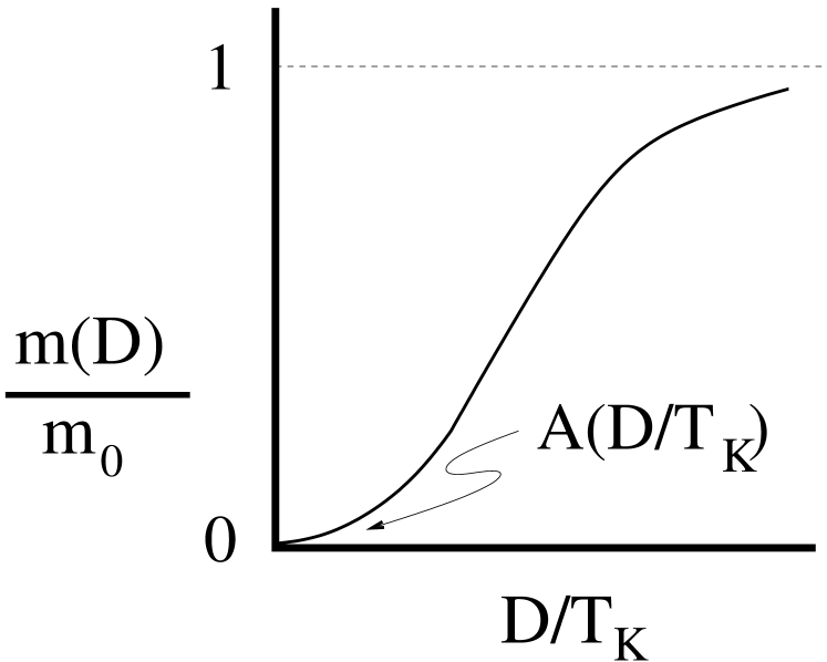
Figure 4: $m(D)$ as a function of $D/T_{K}$: the crossover from the perturbative behavior to the linear dependence on $D/T_{K}$ for $D/t_{K}\ll 1$ is evidenced.

Acknowledgements: We benefited from discussions with A. Trombettoni, R. Egger, A. Ferraz, H. Johannesson, V. Korepin and A. Tagliacozzo. P. S. thanks CNPq for partial financial support through the grant provided by a Bolsa de Produtivitade em Pesquisa.

References

- [1] A. M. Tsvelik, Phys. Rev. Lett. 110, 147202 (2013).
- [2] A. C. Hewson, The Kondo problem to heavy fermions, Cambridge University Press, 1997.
- [3] P. Nozières, Journal of Low Temperature Physics, 17, Nos. 1/2 (1974).
- [4] P. Nozières and A. Blandin, J. Phys. 41, 193 (1980).
- [5] D. Cox and A. Zawadowski, Adv. Phys. 47, 599 (1998).
- [6] N. Andrei and C. Destri, Phys. Rev. Lett. 52, 364 (1984).
- [7] A.M. Tvelick and P. B. Wiegmann, Z. Phys. B 54, 201 (1984).
- [8] I. Affleck, Nucl. Phys. B 336, 517 (1990); I. Affleck and A. Ludwig, Nucl. Phys. B 352, 849 (1991); Nucl. Phys. B 360, 641 (1991).
- [9] D. Giuliano, B. Jouault and A. Tagliacozzo, Europhys. Lett. 58, 401 (2002).
- [10] Y. Oreg and D. Goldhaber-Gordon, Phys. Rev. Lett. 90, 136602 (2003); R. M. Potok, I. G. Rau, H. Shtrikman, Y. Oreg, and D. Goldhaber-Gordon, Nature 446, 167 (2007).
- [11] N. Crampe and A. Trombettoni, Nucl. Phys. B 871, 526 (2013).
- [12] T. Matsubara and H. Matsuda, Prog. Theor. Phys. 16, 416 (1956); Prog. Theor. Phys. bf 16, 569 (1956); Prog. Theor. Phys. 17, 19, (1957).
- [13] J. Simon, W. S. Bakr, R. Ma, M. E. Tai, P. M. Preiss, and M. Greiner, Nature 472, 307 (2011).
- [14] D. Giuliano, D. Rossini, P. Sodano, and A. Trombettoni Phys. Rev. B 87, 035104 (2013).
- [15] D. Giuliano and P. Sodano, Nucl. Phys. B 711, 480 (2005).
- [16] D. B. Haviland, K. Andersson, and P. Agren, J. Low Temp. Phys. 124,(2001) 291.
- [17] D. Giuliano and P. Sodano, New. Jour. of Physics 10,093023(2008).
- [18] D. Giuliano and P. Sodano, Nucl. Phys. B 811, 395 (2009).
- [19] A. Cirillo, M. Mancini, D. Giuliano, and P. Sodano, Nucl. Phys. B 852, 235 (2011).
- [20] V. Rizzi, V. Cataudella, and R. Fazio, Phys.Rev. B 73, 100502 (2006).
- [21] I. V. Protopopov and M. V. Feigel’ man, Phys. Rev.B 70, 184519 (2004);Phys. Rev. B 74, 064516 (2006).
- [22] D. Giuliano and P. Sodano, EPL 88, 17012 (2009)
- [23] D. Giuliano and P. Sodano, Nucl. Phys. B 837, 153 (2010).
- [24] B. Douçot and J. Vidal, Phys. Rev. Lett. 88, 227005 (2002).
- [25] P. Coleman, L. B. Ioffe, and A. M. Tsvelik, Phys. Rev. B 52, 6611 (1995).
- [26] L. I. Glazman and A. I. Larkin,Phys. Rev. Lett. 79, 3736 (1997).
- [27] D. Giuliano and A. Tagliacozzo, Jour. Phys. Cond. Matt. 16, 6075 (2004).
- [28] L.B. Ioffe and M.V. Feigel’man, Phys. Rev. B 71, 024505 (2005).
- [29] I. M. Pop, K. Hasselbach, O. Buisson, W. Guichard, and B. Pannetier, Phys. Rev. B 78, 104504 (2008).