Driving Disk Winds and Heating up Hot Coronae by MRI Turbulence

Abstract

We investigate the formation of hot coronae and vertical outflows in accretion disks by magneto-rotational turbulence. We perform local three-dimensional (3D) MHD simulations with the vertical stratification by explicitly solving an energy equation with various effective ratios of specific heats, $\gamma$. Initially imposed weak vertical magnetic fields are effectively amplified by magnetorotational instability (MRI) and winding due to the differential rotation. In the isothermal case ($\gamma=1$), the disk winds are mainly driven by the Poynting flux associated with the MHD turbulence and show quasi-periodic intermittency. On the other hand, in the non-isothermal cases with $\gamma\geq 1.1$, the regions above 1-2 scale heights from the midplane are effectively heated up to form coronae with the temperature of $\sim$ 50 times of the initial value, which are connected to the cooler midplane region through the pressure-balanced transition regions. As a result, the disk winds are mainly driven by the gas pressure with exhibiting more time-steady nature, although the nondimensional time-averaged mass loss rates are similar to that of the isothermal case. Sound-like waves are confined in the cool midplane region in these cases, and the amplitude of the density fluctuations is larger than that of the isothermal case.

1. Introduction

In accretion disks magnetohydrodynamical (MHD) turbulence is believed to work as effective viscosity and play an essential role in the outward transport of the angular momentum and the radial motion of the gas (e.g. Lynden-Bell & Pringle, 1974; Balbus & Hawley, 1998). Magnetorotational instability (MRI hereafter Velikhov, 1959; Chandrasekhar, 1960; Balbus & Hawley, 1991) is a promising source of such turbulent viscosity in accretion disks.

Properties of the MRI in accretion disks have been widely studied. MHD simulations in the local shearing coordinates (Goldreich & Lynden-Bell, 1965) have been extensively and intensively performed without vertical density stratification (e.g., Hawley et al., 1995; Matsumoto & Tajima, 1995; Sano et al., 2004), and with the vertical stratification due to the gravity by a central object (e.g., Stone et al., 1996; Miller & Stone, 2000; Davis et al., 2010; Shi et al., 2010; Okuzumi & Hirose, 2011; Sai et al., 2013).

Accretion disks threaded with global magnetic fields are supposed to drive disk winds, which was first suggested by Blandford & Payne (1982) as an origin of jets from black hole accretion disks. This picture of magnetocentrifugally driven disk winds was extended to protostellar jets (Pudritz & Norman, 1983). Outflows and jets from various types of accretion disks have been observed, e.g., from young stars (Ohashi et al., 1997; Coffey et al., 2004), and from active galactic nuclei (Tombesi et al., 2010).

These two pictures – MRI-driven turbulence in accretion disks and magnetically driven winds from disk surfaces involving coherent field lines – are supposed to have a close link. For instance, turbulence in disks could drive the vertical motions of the gas by the MHD turbulent pressure. Based on these considerations, Suzuki & Inutsuka (2009) and Suzuki et al. (2010) recently proposed the onset of vertical outflows from MRl-turbulent accretion disks. They performed MHD simulations in local shearing boxes with the vertical stratification and net vertical magnetic fields by taking a special care of the outgoing boundary conditions (Suzuki & Inutsuka, 2006) at the vertical surfaces of the simulation boxes. They found that the disk winds are driven from the upper and lower boundaries by the Poynting flux associated with the MHD turbulence. This process can contribute to the mass loading to the basal regions of the global disk winds introduced above. Such vertical outflows are also observed in 3D global simulations (Flock et al., 2011; Suzuki & Inutsuka, 2013).

Later on, such MRI-turbulent driven disk winds have been further studied from various aspects. Bai & Stone (2013) examined properties of the disk winds with stronger net vertical magnetic fields. The connection between the upflows in local simulations and the global disk winds/jets is investigated (Lesur et al., 2013; Bai & Stone, 2013). Fromang et al. (2013, see also Suzuki & Inutsuka 2010) pointed out the mass flux of the disk winds depends on the simulation box size, which shows that we need great cares to handle disk winds by local shearing boxes.

Although there are limitations in the shearing box approximation, it is still useful technic to study the basic properties of MRI-turbulent driven vertical outflows. Most of previous simulations adopt an isothermal equation of state to mainly focus on the dynamics of the disk winds, apart from a limited number of works that considered detailed heating and cooling processes for black hole accretion disks (Turner, 2004; Hirose et al., 2006) and protoplanetary disks (Hirose & Turner, 2011). So far there has been no systematic studies done for the MRI-turbulent driven winds with different ratios of specific heats, $\gamma$ even within a framework of the shearing box approximation, which is the main focus of the present paper.

2. Simulation Setups

In Suzuki & Inutsuka (2009) & Suzuki et al. (2010) we performed 3D MHD simulations in local stratified shearing boxes (Stone et al., 1996) by solving the ideal MHD equations with an isothermal equation of state. In this paper, we extend these works by explicitly solving an energy equation in a Lagrangian form,

$$\rho\frac{d}{dt}\left[e+\frac{v^{2}}{2}+\frac{B^{2}}{8\pi\rho}+\frac{\Omega^{2}}{2}(z^{2}-3x^{2})\right]$$

$$=\mbox{\boldmath${\nabla}$}\cdot\left[-\left(p+\frac{B^{2}}{8\pi}\right)\mbox{\boldmath${v}$}+\frac{\mbox{\boldmath${B}$}}{4\pi}(\mbox{\boldmath${B\cdot v}$})\right],$$ (1)

where $\Omega$ is the Keplerian rotation frequency, $e$ is the specific energy per mass which is related to the gas pressure, $p$, the density, $\rho$, and the effective ratio of specific heats, $\gamma$, as

$$e=\frac{1}{\gamma-1}\frac{p}{\rho},$$ (2)

and the other variables in Equation (1) have the conventional meanings. The terms involving $\Omega^{2}$ in Equation (1) originate from the central object; $\Omega^{2}z^{2}/2$ is the potential due to the vertical component of the gravity and $-3\Omega^{2}x^{2}/2$ denotes the tidal potential.

In the energy equation above we do not explicitly consider external cooling and heating processes, e.g., radiation cooling/heating, thermal conduction, and etc. Instead, we study their effect phenomenologically by assuming different but spatially uniform $\gamma$ from 1 to $5/3$ in different cases. In our simulations, the gas is heated up mainly by the dissipation of magnetic energy, which we discuss later in this section. Taking $\gamma=1$ (isothermal condition) indicates that we (implicitly) assume that the temperature is kept constant by an unspecified cooling that can balance the magnetic heating. On the other hand, larger $\gamma$ corresponds to suppressing cooling; $\gamma=7/5$ and $5/3$ correspond to the adiabatic conditions for diatomic and monoatomic gases, respectively.

Apart from explicitly solving the energy equation, we basically follow Suzuki & Inutsuka (2009) when performing the numerical simulations. We adopt a second-order Godunov-CMoCCT scheme (Sano et al., 1999), in which we solve the nonlinear Riemann problems with the magnetic pressure at the cell boundaries for the compressive waves and adopt the consistent method of characteristics (CMoC) for the evolution of magnetic fields (Clarke, 1996). At the top and bottom $z$ boundaries, we prescribe the outgoing boundary condition by using the seven MHD characteristics (Suzuki & Inutsuka, 2006).

We fix the ratio of the box sizes of the $x$, $y$, and $z$ axes to 1:4:8, which are respectively resolved by 32, 64, and 256 spatially uniform grids. Each cell is elongated in the $y$ direction with $\Delta y$ being twice as large as $\Delta x$ and $\Delta z$. The lengths in the simulations are normalized by the initial pressure scale heights, $H_{0}$, as

$$H_{0}=\frac{\sqrt{2}c_{\rm s,0}}{\Omega}\equiv\frac{\sqrt{2T_{0}}}{\Omega},$$ (3)

where $c_{\rm s,0}$ is the initial sound speed, and we also use the initial temperature, $T_{0}$, which has the dimension of $v^{2}$. Hereafter subscripts ‘0’ represent the initial state. In this paper, $c_{\rm s}$ stands for an “isothermal” sound speed, $=\sqrt{p/\rho}=\sqrt{T}$; the usual sound speed, $\sqrt{(\partial p/\partial\rho)_{s}}=\sqrt{\gamma p/\rho}=\sqrt{\gamma T}$, is expressed as $\sqrt{\gamma}c_{\rm s}$. We initially set up the hydrostatic density structure with the constant temperature, $T=T_{0}$,

$$\rho=\max\left(\rho_{\rm mid,0}\exp\left(-\frac{z^{2}}{H_{0}^{2}}\right),10^{-9}\rho_{\rm mid,0}\right),$$ (4)

where $\rho_{\rm mid,0}$ is the initial density at the midplane. In order to perform the simulations stably, we adopt a floor value, $\rho_{\rm fl}=10^{-9}\rho_{\rm mid,0}$ throughout the simulations. In the non-isothermal cases, the simulation boxes are larger than that of the isothermal case to treat the extended coronae as shown later. In the cases with $\gamma\geq 1.03$, the initial densities near the surface regions, $|z|>4.55H_{0}$, are smaller than $\rho_{\rm fl}$, hence $\rho_{\rm fl}$ is used for these regions. In the simulations, we use the unit of $\Omega=1$, $H_{0}=1$, and $\rho_{\rm mid,0}=1$; accordingly, $T_{0}=1/2$ and $c_{\rm s,0}=1/\sqrt{2}$. We initially impose the weak net vertical magnetic field, $B_{z,0}$, with the plasma $\beta$ value, $8\pi p_{\rm mid,0}/B_{z,0}^{2}=10^{6}$ at the midplane. We start the simulations with giving small random perturbations with 0.5% of $c_{\rm s,0}$ as seeds of the MRI. The simulations are kept running until 200 rotations ($t\Omega/2\pi=200$).

In the simulations with $\gamma>1$, the gas is heated by the dissipation of the magnetic energy, where the heating is done by the numerical effect in the sub-grid scale since we do not explicitly take into account resistivity. Physically, we expect that the heating is due to cascading turbulence at small scales. As a disk is heated up, the sound speed increases, and accordingly the pressure scale height also increases. Therefore, to study the vertical structure, the $z$ coordinate in units of the scale height,

$$\int_{0}^{z}\frac{dz}{\langle h(z)\rangle}_{x,y}\equiv\int_{0}^{z}\frac{dz\Omega}{\sqrt{2}\langle c_{\rm s}\rangle_{x,y}(z)},$$ (5)

is a key quantity, where the subscripts, $x,y$, of $\langle\;\rangle$ indicate the average over a horizontal ($x-y$) plane. While $\int_{0}^{z}\frac{dz}{\langle h(z)\rangle_{x,y}}=z/H_{0}$ for the isothermal situation, generally $|\int_{0}^{z}\frac{dz}{\langle h(z)\rangle_{x,y}}|<|z/H_{0}|$ as a result of the heating for $\gamma>1$.

Table 1Simulation runs with different ratios of specific heats, $\gamma$.

$\gamma$	$(X,Y,Z)/H_{0}$	$\int_{z_{\rm bot}}^{z_{\rm top}}{dz}{\langle h(z)\rangle}$	$\Delta t_{\rm ave}$(rot.)	$M_{\rm f}/M_{0}$
1.0	0.9,3.6,7.2	7.2	140–200	0.907
1.01	1.0,4.0,8.0	7.1	120–200	0.895
1.03	1.35,5.4,10.8	7.1	100–200	0.896
1.1	4.0,16.0,32.0	7.3	150–200	0.951
1.2	4.0,16.0,32.0	7.1	130–200	0.906
1.3	4.0,16.0,32.0	7.3	130–200	0.937
1.4	4.0,16.0,32.0	7.4	120–200	0.934
5/3	4.0,16.0,32.0	7.2	120–200	0.890

Note. — The initial box size (2nd column) and the final vertical box size measured in the final scale height (3rd column; Equation 6) averaged over $\Delta t_{\rm ave}$ are compared. $X$ ,$Y$, and $Z(=z_{\rm top}-z_{\rm bot})$ in the 2nd column are the sizes of $x$, $y$, and $z$ components of the simulation box. The 4th column shows the final mass, $M_{\rm f}$, normalized by the initial mass, $M_{0}$, remained in the box.

The mass flux of the disk winds depends on the vertical box size in units of the scale height (Suzuki et al., 2010; Fromang et al., 2013). In order to compare the properties of the disk winds with different $\gamma$, it is desirable to adopt the same vertical box size in units of the final scale height after the steady-state conditions are achieved,

$$\int_{z_{\rm bot}}^{z_{\rm top}}\frac{dz}{\langle h(z)\rangle_{\Delta t_{\rm ave},x,y}},$$ (6)

where $z_{\rm bot}$ and $z_{\rm top}$ indicate the locations of the bottom and top boundaries of the simulation box, and we take the average over $\Delta t_{\rm ave}$ (Table 1) after the magnetic fields are amplified to the saturated state, which we describe later in this section. We cannot estimate $h(z)$ in advance, hence we perform simulations with different box sizes and pick up one that gives the desirable value for each $\gamma$. For the isothermal case ($\gamma=1$), we fix the vertical box size $(z_{\rm top}-z_{\rm bot})=7.2H_{0}$, indicating $0.9H_{0}$ and $3.6H_{0}$ for the box sizes in the $x$ and $y$ directions. For the other cases with $\gamma>1$, we tune the initial box sizes to give the final vertical box sizes after the saturation in a range of $7.1<\int_{z_{\rm bot}}^{z_{\rm top}}dz/\langle h(z)\rangle_{\Delta t_{\rm ave},x,y}<7.4$.

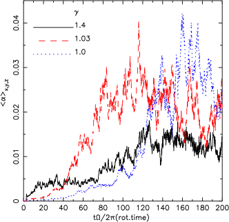
Figure 1.— Evolution of the box-averaged $\langle\alpha\rangle_{x,y,z}$ of the three cases with $\gamma=1.4$ (black solid), 1.03 (red dashed), and 1.0 (blue dotted). The vertical axis, $t\Omega/2\pi$, indicates time in units of one rotation.

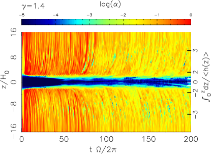
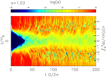
Figure 2.— Time-distance diagrams of $\langle\alpha\rangle_{x,y}$ of the cases with $\gamma=1.4$ (top), 1.03 (middle) and 1.0 (lower). The horizontal axis ($t\Omega/2\pi$) denotes time in units of rotation. The vertical axis shows $z$; on the left shown is distance in units of the initial scale height, $z/H_{0}$, and on the right shown is distance in units of the final scale height, $\int_{0}^{z}dz/\langle h(z)\rangle_{\Delta t_{\rm ave},x,y}$.

In order to check the saturation of the magnetic fields, we monitor the box-averaged $\alpha$ values (Shakura & Sunyaev, 1973), which is the sum of the Reynolds and Maxwell stresses normalized by the gas pressure,

$$\langle\alpha\rangle_{x,y,z}=\frac{\int_{z_{\rm bot}}^{z_{\rm top}}dz\langle\rho v_{x}\delta v_{y}-B_{x}B_{y}/4\pi\rangle_{x,y}}{\int_{z_{\rm bot}}^{z_{\rm top}}dz\langle p\rangle_{x,y}},$$ (7)

where $\delta v_{y}=v_{y}-v_{y,0}$ is the difference of toroidal velocity from the Keplerian shear flow, $v_{y,0}=-\frac{3}{2}\Omega x$. In Figure 1 we show the results of the cases with $\gamma=1.4$ (black solid line), 1.03 (red dashed line), and 1.0 (blue dotted line). We also display the time evolution of the vertical structure of horizontally averaged $\langle\alpha\rangle_{x,y}=\langle\rho v_{x}\delta v_{y}-B_{x}B_{y}/4\pi\rangle_{x,y}/\langle p\rangle_{x,y}$ in $t$–$z$ diagrams in Figure 2 to see more details. In the case with $\gamma=1.4$, the saturation is observed after $t\Omega/2\pi\gtrsim 120$, and we use $\Delta t_{\rm ave}=120-200$ rotations (1 rotation$=2\pi/\Omega$) to estimate the vertical box size in the final scale height (Equation 6). Although in the case with $\gamma=1.03$ the box averaged $\langle\alpha\rangle_{x,y,z}$ almost saturates after $t\Omega/2\pi\gtrsim 80$ (Figure 1), we use a more conservative $\Delta t_{\rm ave}=100-200$, because $\langle\alpha\rangle_{\Delta t_{\rm ave},x,y}$ at the midplane is growing in $t\Omega/2\pi\lesssim 90$ (middle panel of Figure 2). In the isothermal case ($\gamma=1.0$), we use $\Delta t_{\rm ave}=140-200$ rotations, because $\langle\alpha\rangle_{x,y,z}$ becomes saturated later than in the other two cases. On the right of each panel of Figure 2, we show $z$ in units of the final scale height, $\int_{0}^{z}dx/\langle h(z)\rangle_{\Delta t_{\rm ave},x,y}$. The interval between the ticks with $\Delta z=1$ varies with height in the non-isothermal cases because the temperature is higher near the surfaces as shown in $\S$ 3.

The initial and final box sizes and $\Delta t_{\rm ave}$’s are summarized in Table 1. For the cases with $\gamma\geq 1.1$, the vertical box size measured in the final scale height shrinks more than a factor of 4 because of the heating, which we examine in §3. The derived $\Delta t_{\rm ave}$ is also used to examine the time-averaged vertical structures of each case in §3.

The horizontal box sizes measured in the scale height of the non-isothermal cases vary with height because of the variation of the temperature. Because of the higher temperature near the surfaces (§3), the horizontal box sizes in units of the final scale height, $\int_{x_{\rm min}}^{x_{\rm max}}dx/\langle h(z)\rangle_{\Delta t_{\rm ave},x,y}<0.9$ and $\int_{y_{\rm min}}^{y_{\rm max}}dy/\langle h(z)\rangle_{\Delta t_{\rm ave},x,y}<3.6$, are smaller in the surface regions. of the non-isothermal cases. Although these horizontal sizes are insufficient to quantitatively discuss the saturation of the magnetic fields (e.g., Guan et al., 2009), we anticipate that it is still meaningful to compare the vertical disk structures with different $\gamma$.

3. Results

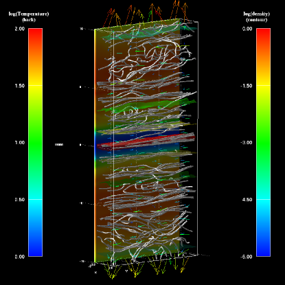
Figure 3.— Snapshot of the simulation with $\gamma=1.4$ at 180 rotation time ($t\Omega/2\pi=180$). White lines indicate magnetic field lines, colors on the back show normalized temperature, $T/T_{0}$, (left legend), color contours denote iso-density surfaces (right legend), and arrows indicate velocity fields.

Continued from the previous section we examine the time evolutions of the box averaged $\langle\alpha\rangle_{x,y,z}$ in Figure 1. After the quasi-steady saturated states are achieved, the three cases show different behavior. The isothermal case ($\gamma=1.0$) show large fluctuations of $\langle\alpha\rangle_{x,y,z}$ from 0.015 to 0.04. On the other hand, the case with $\gamma=1.4$ exhibits much milder behavior with $\langle\alpha\rangle_{x,y,z}$ kept in a range of 0.01-0.015. The case with $\gamma=1.03$ shows intermediate behavior; although the increase of the $\alpha$ is faster with showing large fluctuations in the earlier time, $2\pi t/\Omega\lesssim 120$, it settles down to a softer state later, between those for $\gamma=1.4$ and 1.0. Interestingly enough, the similar trends are observed in the disk winds, which we discuss the details in §3.3.

Figure 3 exhibits a snapshot structure of the case with $\gamma=1.4$ at 180 rotation time ($t\Omega/2\pi=180$). The turbulent magnetic field, mostly dominated by the toroidal component, is amplified by MRI and winding due to the differential rotation. The temperature contour on the back shows that the temperatures in $4\lesssim|z/H_{0}|\lesssim 12$ increase up to more than 50 times of the initial value, while the temperature in the midplane does not increase so much. $\frown$-shaped field lines, which are typical for Parker (magnetic buoyancy) instability (Parker, 1955; Nishikori et al., 2006) are seen in the surface regions, and the vertical outflows are observed from both the upper and lower surfaces, similarly to those seen in the isothermal simulations (Suzuki & Inutsuka, 2009; Suzuki et al., 2010).

3.1. Coronae

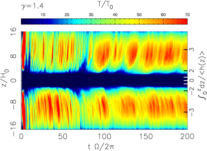
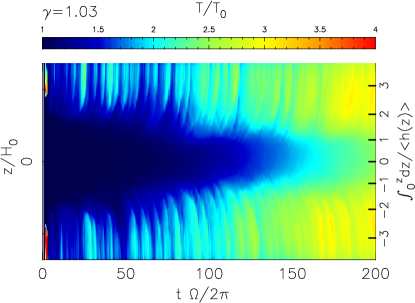
Figure 4.— Time-distance diagrams of temperatures, $\langle T/T_{0}\rangle_{x,y}$, of the cases with $\gamma=1.4$ (upper) and 1.03 (lower). The labels for the horizontal and vertical axes are the same as in Figure 2.

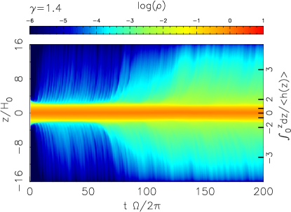
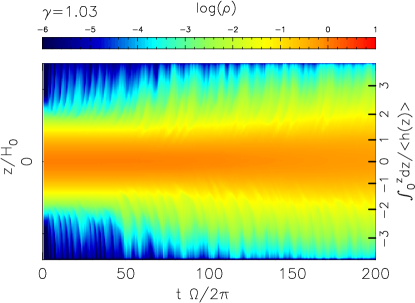
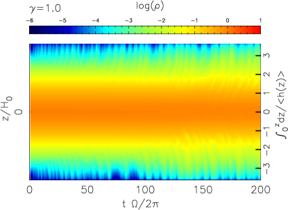
Figure 5.— Time-distance diagrams of densities, $\langle\rho\rangle_{x,y}$, of the cases with $\gamma=1.4$ (top), 1.03 (middle), and 1.0 (bottom). The labels for the horizontal and vertical axes are the same as in Figure 2.

Figures 4 and 5 present $t$–$z$ diagrams of the temperatures and the densities of the three cases with $\gamma=1.4,1.03$, & 1.0, whereas we do not show the temperature of the isothermal ($\gamma=1.0$) case. As shown in Figure 4 as well as Figure 3, the gas in the surface regions of the non-isothermal cases is heated up. The heating is done by the dissipation of the magnetic energy which is amplified by the MRI and the winding due to the differential rotation. Since the simulations do not explicitly take into account resistivity, the dissipation of the magnetic field occurs numerically in the sub-grid scales, whereas we expect that this actually takes place by cascading of small-scale turbulence.

The two cases of Figure 4 show an initial temperature rise in $t\Omega/2\pi<5$, because the initial densities in the upper regions, $|z/H_{0}|>4.55$, are larger than the hydrostatic value (Equation 4); the gas initially flows down from there toward the midplane, which causes the initial heating. The entire region is eventually relaxing to the quasi-steady state, which we analyze from now. In both the cases, the regions of $2.5<|\int_{0}^{z}\frac{dz}{\langle h(z)\rangle}_{\Delta t_{\rm ave},x,y}|<3$ are most effectively heated up to $T/T_{0}\sim 60$ in the case with $\gamma=1.4$ and $T/T_{0}\sim 3$ in the case with $\gamma=1.03$. Because the heating is done by the dissipation of the magnetic field which is amplified by the MRI and the winding, the increase of the temperature follows the increase of $\langle\alpha\rangle_{x,y}$ shown in Figure 2. This is more easily seen in the case with $\gamma=1.03$; the temperature increases in $t\Omega/2\pi\gtrsim 150$, which is delayed compared to the increase of $\langle\alpha\rangle_{x,y}$.

The top panel of Figure 4 illustrates that the hot regions with $T/T_{0}>50$ are clearly separated from the cool midplane region with $T/T_{0}\ll 10$ by the transition regions located at $\int_{0}^{z}\frac{dz}{\langle h(z)\rangle_{\Delta t_{\rm ave},x,y}}\approx\pm 1.5$; from now we call these hot regions coronae. On the other hand, in the small $\gamma$ ($=$1.03) case, the temperatures of the surface regions are not so high with $T/T_{0}\approx 3$ in the upper regions.

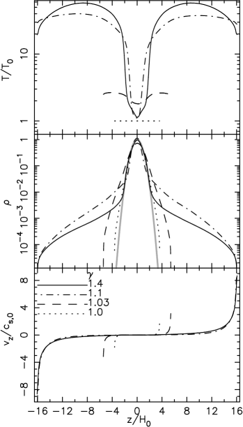
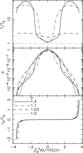
Figure 6.— Comparison of the time and horizontally averaged vertical structures of the cases with $\gamma=1.4$ (solid), 1.1 (dot-dashed), 1.03 (dashed), and 1.0 (dotted). The horizontal axis is vertical distance in units of the initial scale height $z/H_{0}$ for the left panels and in units of the final scale heights, $\int_{0}^{z}dz/\langle h(z)\rangle_{\Delta t_{\rm ave},x,y}$, for the right panels. From top to bottom, the temperatures normalized by the initial value, the densities, and the vertical velocities normalized by the initial constant sound speed, $c_{\rm s,0}$, (left panels) or normalized by the final local sound speeds, $c_{\rm s}(z)$, (right panels) are compared. The gray thick lines in the middle panels indicate the initial density profile.

For more quantitative inspection we display the time and horizontally averaged vertical structures of the four cases, $\gamma=1.0,1.03,1.1$, & 1.4 in Figure 6, where the time averages are taken over $\Delta t_{\rm ave}$ in Table 1 after the quasi-steady saturation is achieved (Figure 1). The top panel illustrates that the coronae with $T/T_{0}\approx 40$ also form in the case with $\gamma=1.1$. We have found that the formation of the coronae with $T/T_{0}\approx 40-70$ is universal in the cases with $\gamma\geq 1.1$. In these cases, with the large increases of the temperature (around $\int_{0}^{z}dz/\langle h(z)\rangle_{\Delta t_{\rm ave},x,y}\approx\pm 1.5$ for $\gamma=1.4$ and $\pm 1$ for $\gamma=1.1$) the density (middle panels) rapidly decreases to keep the nearly pressure-balanced structure. We call this pressure balanced structure with temperature rise a transition region.

The existence of the hot coronae above the cool midplane region is quite different from some results of recent stratified shearing box simulations. For instance, Bodo et al. (2012) performed the simulations with fixing the temperatures to the initial value ($T=T_{0}$) and the velocities to zero ($v_{z}=0$) at the top and bottom $z$ boundaries. They showed that the maximum temperature is obtained at the midplane and the temperature monotonically decreases to the surfaces. This shows that the boundary condition at the $z$ boundaries play a significant role in the vertical temperature and velocity structures.

Coupled with the formation of the hot coronae ($\gamma\geq 1.1$) or the warm regions ($1<\gamma<1.1$), the gas is lifted up from the midplane region to the upper regions as shown in Figure 5. In the case with $\gamma=1.4$ (top panel), it is clearly seen that the coronae are gradually filled with denser material in $t\Omega/2\pi\gtrsim 50$ by the evaporation from the midplane region, and at later times the evaporated gas is mainly supported by the gas pressure of the hot coronae (§3.3). The time averaged density structures of the cases $\gamma=1.1$ and 1.4 (middle panels of Figure 6) quantitatively show the large uplifted gas compared with the initial hydrostatic profile with the constant $T_{0}$ (gray thick lines). The supply of the gas to the coronal regions is also seen in the case with $\gamma=1.03$ (middle panel of Figure 5) although the amount is smaller than those of larger $\gamma$ cases. Even in the isothermal case (bottom panel of Figure 5) quasi-periodic uplifting motions of the gas are observed, which are by the Poynting flux associated with the breakups of channel flows (Suzuki & Inutsuka, 2009). The uplifted gas is finally connected to disk winds as will be discussed in §3.3.

3.2. Saturation of Magnetic Field

Figure 7.— Comparison of the time and horizontally averaged vertical structures of the $i=x$ (top), $y$ (middle), and $z$ (bottom) components of magnetic energies, $B_{i}^{2}/8\pi$, normalized by the initial gas pressure at the midplane, $p_{\rm 0,mid}$ (left), and quality factors, $Q_{i}$, for MRI (right) of the cases with $\gamma=1.4$ (solid), 1.1 (dot-dashed), 1.03 (dashed), and 1.0 (dotted). The horizontal axis, $\int_{0}^{z}dz/\langle h(z)\rangle_{\Delta t_{\rm ave},x,y}$, is measured in the final scale heights.

Figure 8.— Comparison of the time and horizontally averaged vertical structures of the plasma $\beta$ values (upper) and the $\alpha$ values (bottom) of the cases with $\gamma=1.4$ (solid), 1.1 (dot-dashed), 1.03 (dashed), and 1.0 (dotted). The horizontal axis, $\int_{0}^{z}dz/\langle h(z)\rangle_{\Delta t_{\rm ave},x,y}$, is measured in the final scale heights.

Magnetic field plays a central role in the formation of the coronae because its dissipation leads to the heating. The left panels of Figure 7 compare the time and horizontally averaged magnetic energies of the four cases with $\gamma=1.4$, 1.1, 1.03, and 1.0. The toroidal ($y$) component dominates as expected because of the winding by the differential rotation. In the surface regions, $|\int_{0}^{z}dz/\langle h(z)\rangle_{\Delta t_{\rm ave},x,y}|\gtrsim 2$, these four cases show similar profiles one another. On the other hand, in the midplane region larger $\gamma$ cases give lower magnetic energies of the $x$ and $z$ components in particular. $B_{y}^{2}$ only weakly depends on $\gamma$ because the strength of $B_{y}$ is mostly controlled by the winding. As a result, in the midplane region of larger $\gamma$ cases more or less coherent toroidal magnetic field dominates (Figure 3).

The lower levels of $B_{x}^{2}$ and $B_{z}^{2}$ are mainly because of the insufficient resolution. The right panels of Figure 7 display the time and horizontally averaged $i$-th components ($i=x,y,z$) of quality factors with respect to MRI (Noble et al., 2010; Hawley et al., 2011),

$$Q_{i}=2\pi\frac{\sqrt{v_{{\rm A},i}^{2}}}{\Omega\Delta l_{i}}=2\pi\sqrt{\frac{B^{2}_{i}}{4\pi\rho}}\frac{1}{\Omega\Delta l_{i}},$$ (8)

where $v_{{\rm A},i}=B_{i}/\sqrt{4\pi\rho}$ is Alfvén velocity along with an $i$–th direction and $\Delta l_{i}(=\Delta x,\Delta y\Delta z)$ is the grid size of an $i$–th component. $Q_{i}$ measures the number of mesh points which resolves the most unstable wavelength of MRI. According to Sano et al. (2004), $Q_{z}\gtrsim 6$ is a necessary condition for a vertical magnetic field to get a linear growth rate close to the analytic prediction from MRI. $Q_{x}$ and $Q_{z}$ of the cases with $\gamma=1.4$ and 1.1 at the midplane is small $<5$. In these cases the initial scale height, $H_{0}$, is resolved by 8 mesh points. Although at later time one scale height, $h(z)$, is eventually resolved by a larger number of grids, $\sim 10-15$, it is still insufficient to capture fine turbulent structure by the MRI at the midplane (Simon et al., 2009; Hawley et al., 2011, 2013; Parkin & Bicknell, 2013a, b). Therefore, the magnetic field strength at the midplane in the large $\gamma\geq 1.1$ is supposed to be underestimated and not to develop to the physically saturated state. On the other hand, in the small $\gamma<1.1$ cases and the surface regions of the large $\gamma$ cases we can safely discuss the saturation of the magnetic fields.

Figure 8 displays the time and horizontally averaged plasma $\beta$ values,

$$\langle\beta\rangle_{\Delta t_{\rm ave},x,y}=\frac{8\pi\langle p\rangle_{\Delta t_{\rm ave},x,y}}{\langle B^{2}\rangle_{\Delta t_{\rm ave},x,y}}$$

(upper panel) and $\alpha$ values,

$$\langle\alpha\rangle_{\Delta t_{\rm ave},x,y}=\frac{\langle\rho v_{x}\delta v_{y}-B_{x}B_{y}/4\pi\rangle_{\Delta t_{\rm ave},x,y}}{\langle p\rangle_{\Delta t_{\rm ave},x,y}}$$

(lower panel). $\langle\beta\rangle_{t_{\rm ave},x,y}$ is larger and $\langle\alpha\rangle_{t_{\rm ave},x,y}$ is smaller for smaller $\gamma$. In the surface regions, this is explained by the larger gas pressure due to the hotter coronae for larger $\gamma$ since the magnetic field strengths are similar among different $\gamma$ cases (left panels of Figure 7). The large $\beta$ and small $\alpha$ values at the midplane region in the cases with $\gamma=1.4$ and 1.1 are mainly because of the weaker magnetic field strength owing to the insufficient resolution (Figure 7).

In the surface regions, $|\int_{0}^{z}dz/\langle h(z)\rangle_{\Delta t_{\rm ave},x,y}|\gtrsim 2$, the $\langle\beta\rangle_{\Delta t_{\rm ave},x,y}$ values of the different cases are almost spatially constant (Figure 8), which indicates that the magnetic energy decreases with increasing $|z|$ (left panels of Figure 7) in the same manner as the decrease of the gas pressure, whereas the level of $\langle\beta\rangle_{\Delta t_{\rm ave},x,y}$ depends on $\gamma$ reflecting the coronal gas pressure in the numerator of $\beta$. In other words, the magnetic energy dissipates in these surface regions; the magnetic energy becomes relatively important with an elevating altitude from the midplane with decreasing density, and at the locations, $\int_{0}^{z}dz/\langle h(z)\rangle_{\Delta t_{\rm ave},x,y}\approx\pm 2$, with $\rho\approx$ $10^{-2}$–$10^{-3}$ times $\rho_{\rm mid}$ (Figure 6) and $1\lesssim\beta<10$, i.e., nearly equipartition, the magnetic energy starts to be gradually converted to other forms. This is the source of the coronal heating and the driving of the disk winds. Although in our simulations the dissipation of the magnetic energy is due to numerical dissipation at the sub-grid scales, in reality the MHD turbulence is supposed to dissipate through the energy cascading to smaller scales.

3.3. Vertical Outflows

Figure 9.— Comparison of the time and horizontally averaged vertical structures of the gas pressure (dashed), the magnetic pressure (dotted), and the magnetic tension (solid) terms of the cases with $\gamma=1.4$ (left), 1.03 (middle), and 1.0 (right). See text (Equations 9 & 10 and their explanations) for details.

The bottom panels of Figure 6 show that vertical outflows are accelerated in the surface regions. The left bottom panel ($v_{z}/c_{\rm s,0}$–$z/H_{0}$) shows that in larger $\gamma$ cases faster outflows are driven at higher altitudes. This is because the material is more extended to higher altitudes and the winds are effectively accelerated by the gas pressure of the hotter gas. If we plot the same quantity in the $v_{z}/c_{\rm s}(z)$–$\int_{0}^{z}dz/\langle h(z)\rangle_{\Delta t_{\rm ave},x,y}$ diagram (right bottom panel), the profiles of the shown four models resemble one another; the vertical velocities reach the local sound speeds at $\int_{0}^{z}dz/\langle h(z)\rangle_{\Delta t_{\rm ave},x,y}\approx\pm 3.5$ where the densities decrease to $\sim 10^{-4}-10^{-5}$ times $\rho_{\rm mid}$. By these outflows, the total mass in the simulation box of each case gradually decreases with time. Typically 5-10 % of the initial mass is lost until the end of the simulations at $t\Omega/\pi=200$ rotations (Table 1).

We inspect how the driving mechanism of these disk winds is different for different $\gamma$. By rearranging Equation (1), we can derive an Eulerian form of the energy equation:

$$\frac{\partial}{\partial t}\left[\rho\frac{v^{2}}{2}+\rho e+\frac{B^{2}}{8\pi}+\rho\Psi\right]$$ (9)

$$= -\mbox{\boldmath${\nabla\cdot}$}\left[\rho\mbox{\boldmath${v}$}\left(\frac{v^{2}}{2}+h+\Psi\right)-\frac{1}{4\pi}(\mbox{\boldmath${v\times B}$})\mbox{\boldmath${\times B}$}\right]$$

$$= -\mbox{\boldmath${\nabla\cdot}$}\left[\left\{\mbox{\boldmath${v}$}\left(\rho\frac{v^{2}}{2}+\rho e+\frac{B^{2}}{8\pi}+\rho\Psi\right)\right\}\right.$$

$$\left.+\left\{\left(p+\frac{B^{2}}{8\pi}\right)\mbox{\boldmath${v}$}-\frac{\mbox{\boldmath${B}$}}{4\pi}(\mbox{\boldmath${B\cdot v}$})\right\}\right],$$

where $\Psi\equiv\frac{\Omega^{2}}{2}(z^{2}-3x^{3})$ and $h=e+p/\rho$. One can see from the last equality, the energy flux can be divided into the two parts; the first $\{\;\}$ bracket indicates the energy advected with ${v}$ and the second $\{\;\}$ bracket indicates the work acting on gas; the second part exactly appears in the spatial derivative term in the Lagrangian form (Equation 1). Here, we examine this work component in the simulations. The $z$ component of the second part can be explicitly written as

$$\left(p+\frac{B^{2}}{8\pi}\right)\mbox{\boldmath${v}$}-\frac{\mbox{\boldmath${B}$}}{4\pi}(\mbox{\boldmath${B\cdot v}$})$$

$$=pv_{z}+\frac{B_{\perp}^{2}}{8\pi}v_{z}-\frac{B_{z}}{4\pi}B_{\perp}v_{\perp}-\frac{B_{z}^{2}}{8\pi}v_{z},$$ (10)

where $B_{\perp}^{2}=B_{x}^{2}+B_{y}^{2}$ and $B_{\perp}v_{\perp}=B_{x}v_{x}+B_{y}v_{y}$. The first, second, and third terms indicate the work by gas pressure, magnetic pressure, and magnetic tension, respectively. The last term is canceled out by a term from the advection component. We compare the first – third terms of the three cases with $\gamma=1.4$ (left panel), 1.03 (middle panel), and 1.0 (right panel) in Figure 9.

If a line in Figure 9 decreases with increasing $z$ in the $z>0$ region, the force acts on gas to drive a vertical upflow, and vice versa in the $z<0$ region. In the isothermal ($\gamma=1.0$) case, the magnetic pressure (dotted line) and tension (solid line) comparably contribute to driving the vertical outflows, while the contribution from the gas pressure is quite small. The “injection regions” of the magnetic tension form around $\int_{0}^{z}dz/\langle h(z)\rangle_{\Delta t_{\rm ave},x,y}\approx\pm 1.5$ as pointed out by Suzuki & Inutsuka (2009); from these regions, the Poynting fluxes associated with the tension are injecting toward both the midplane and surface directions.

On the other hand, in the case with $\gamma=1.4$, the gas pressure largely dominates the magnetic components in driving the disk winds. In this case, the magnetic energy in low-altitude regions once dissipates to heat up the gas. The gas pressure, which increases owing to the magnetic heating, finally contributes to driving the vertical outflows. This is in contrast to the isothermal case, in which the magnetic forces directly drive the vertical outflows. The behavior of the case with $\gamma=1.03$ lies between the two cases. While the largest contribution is from the magnetic pressure, the magnetic tension and the gas pressure also play a significant role.

Inspecting all the cases with different $\gamma$, we can conclude the following results on the driving mechanisms of the disk winds: While in the isothermal and small $\gamma\lesssim 1.03$ cases the vertical outflows are mainly driven by the Poynting flux, in the large $\gamma\gtrsim 1.1$ cases the gas pressure dominantly drives the vertical outflows. However, we should note that, even in the large $\gamma$ cases the magnetic fields play an important role, because the gas pressure is maintained by the dissipation of the magnetic energy which is amplified by the MRI and the winding due to the differential rotation. Since the disk winds are driven from the surface regions where the MRI is well-captured, increasing the numerical resolution does not change the obtained properties of the disk winds so much, although the magnetic field at the midplane of the large $\gamma$ cases would be affected because the numerical resolution there is insufficient at the moment (Figure 7).

Magnetic buoyancy (Parker, 1955) is also considered to operate in the surface regions and contribute to the outflows (Nishikori et al., 2006; Machida et al., 2013). As discussed in Figure 3, $\frown$–shaped field lines, typical for the Parker instability, are sometimes observed. Compared to the isothermal (see also Suzuki et al., 2010) and small $\gamma$ cases, however, the contribution from the magnetic buoyancy is smaller in the large $\gamma$ cases. In general, the Parker instability sets in for magnetically dominated (small $\beta$) condition with strong stratification (short pressure scale height). In the large $\gamma\geq 1.1$ cases the time and horizontally averaged $\beta$ is not so small $\approx 5$ (Figure 8) and the scale height in the surface regions is not short, which tend to suppress the Parker instability compared to the small $\gamma$ cases.

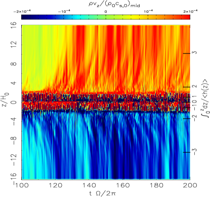
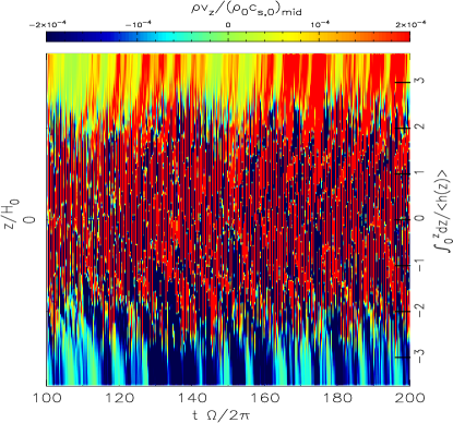
Figure 10.— Time-distance diagrams of the normalized mass flux, $\rho v_{z}/(\rho_{0}c_{\rm s,0})_{\rm mid}$ of the cases with $\gamma=1.4$ (upper) and 1.0 (lower). The labels for the horizontal and vertical axes are the same as in Figure 2.

The difference of the driving mechanisms influences the time-dependency of the disk winds. Figure 10 compares the $t-z$ diagrams of the mass flux of the cases with $\gamma=1.4$ (upper panel) and 1.0 (lower panel). The two cases show quite different appearances. The isothermal case (lower panel) shows a clearer on-off nature of the disk winds. As reported in Suzuki & Inutsuka (2009), it is related to the quasi-periodic breakups of channel-mode flows with 5-10 rotation times. In the case with $\gamma=1.4$, the mass flux increases to the saturated value in $t\Omega/2\pi\gtrsim 120$, after the gas is supplied to the coronal regions (top panel of Figure 5). After that $\rho v_{z}$ exhibits smoother structure in the coronal regions, $|\int_{0}^{z}dz/\langle h(z)\rangle_{\Delta t_{\rm ave},x,y}|>1.5$, with rather quasi-steady vertical outflows. The midplane region ($|\int_{0}^{z}dz/\langle h(z)\rangle_{\Delta t_{\rm ave},x,y}|<1.5$) with $T/T_{0}<10$ (Figure 6) seems to be separated from the coronal regions by the transition regions at $\int_{0}^{z}dz/\langle h(z)\rangle_{\Delta t_{\rm ave},x,y}\approx\pm 1.5$. The quasi-steady nature of the disk winds in this case is related to the fact that the vertical outflows are mainly driven by the gas pressure. The coronal temperatures are more or less uniformly distributed in $|\int_{0}^{z}dz/\langle h(z)\rangle_{\Delta t_{\rm ave},x,y}|\gtrsim 2$, and the force by the gas pressure gradient are more time-steady, which is in contrast to the strong intermittency of the Poynting flux-driven outflows in the isothermal case.

3.4. Dependence on $\gamma$

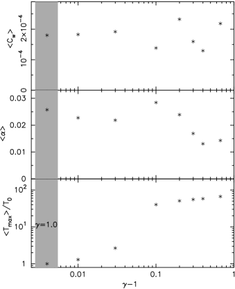
Figure 11.— Dependences of time averaged three quantities on $\gamma-1$. Shown are the sum of the nondimensionalized mass flux of the vertical outflows, $\langle C_{\rm w}\rangle_{\Delta t_{\rm ave},x,y}$, from the upper and lower surfaces (eq.11; top), the peak temperature, the sum of the box-averaged Maxwell and Reynolds stresses, $\langle\alpha\rangle_{\Delta t_{\rm ave},x,y,z}$, (middle), and $\langle T_{\rm max}\rangle_{\Delta t_{\rm ave},x,y}$ (bottom). In the shaded region at the left most location the results of the isothermal case ($\gamma=1.0$) are plotted.

We summarize typical time-averaged quantities of the simulations with different $\gamma$. The top panel of Figure 11 shows the dependence of the mass flux of the disk winds. The shown quantity is

$$\langle C_{\rm w}\rangle_{\Delta t_{\rm ave},x,y}=\left[\langle(\rho v_{z})_{\rm top}\rangle+\langle(-\rho v_{z})_{\rm bot}\rangle\right]/\langle(\rho c_{\rm s})_{\rm mid}\rangle,$$ (11)

where the subscripts, ‘top’ and ‘bot’, indicates the top and bottom boundaries of the simulation box, and the subscript ‘mid’ stands for the midplane. The variables in the brackets on the right hand side are also time and horizontally averaged. The meaning of Equation (11) would be clear, the sum of the mass fluxes from the upper and lower simulation boundaries, which is further normalized by the time and horizontally averaged $\rho c_{\rm s}$ at the midplane. Note that the $-$ sign for the mass flux from the bottom surface is to pick up the outflowing direction.

The data points show that the nondimensional mass flux, $C_{\rm w}$, seems to be almost independent from $\gamma$ and is distributed within a factor of 2, which is consistent with the trend obtained from the time-averaged vertical structure (bottom right panel of Figure 6). This indicates that the time-averaged $C_{\rm w}$ dose not depend on the properties of the vertical outflows, either Poynting flux-driven winds with strong intermittency (smaller $\gamma$) or more time-steady gas pressure-driven wind (larger $\gamma$), which is a little surprising. We suppose that the main reason of the insensitive $C_{\rm w}$ to $\gamma$ is that the original source of the vertical outflows is the magnetic energy. As discussed in §3.2 the magnetic energy gradually dissipates to be converted to other forms of energies at the locations, $\int_{0}^{z}dz/\langle h(z)\rangle_{\Delta t_{\rm ave},x,y}\approx\pm 2$, which is almost independent from $\gamma$, with $\rho\approx$ $10^{-2}$–$10^{-3}$ times $\rho_{\rm mid}$ (Figure 6) and $1\lesssim\beta<10$ (nearly equipartition; Figure 8) .

In the small $\gamma$ regime the magnetic pressure and tension directly accelerate the Poynting flux-driven vertical outflows, while in the large $\gamma$ regime the magnetic energy is firstly transferred to the internal energy, the coronal heating in other words, and then the disk winds are driven by the gas pressure of the hot coronae. The locations (at $\rho\approx 10^{-2}-10^{-3}\rho_{\rm mid}$) of the energy conversion regulate the final mass flux, $C_{\rm w}\approx 2\times 10^{-4}$, which is insensitive to $\gamma$.

The relative comparison of $C_{\rm W}$ among different $\gamma$ cases of the simulations is meaningful since the vertical box sizes are tuned to give 7.1–7.4 in units of the final scale heights (Table 1). However, we should cautiously note that the absolute values of $C_{\rm W}$ should be taken with cares because they depend on the vertical box sizes (Suzuki et al., 2010; Fromang et al., 2013); a larger vertical box would give a smaller $C_{\rm W}$.

The middle panel of Figure 11 presents the box- and time-averaged $\langle\alpha\rangle_{\Delta t_{\rm ave},x,y,z}$ values. We do not find any monotonic trend of $\langle\alpha\rangle_{\Delta t_{\rm ave},x,y,z}$ with $\gamma$ and the values are typically $(1-3)\times 10^{-2}$. However, we cannot proceed detailed saturation arguments (e.g. Simon et al., 2009; Hawley et al., 2011; Parkin & Bicknell, 2013a), since the numerical resolution is not sufficient particularly in the midplane region of the large $\gamma$ cases (right panels of Figure 7).

The bottom panel of Figure 11 compares the maximum temperatures, $T_{\rm max}$, normalized by the initial value, $T_{0}$, of the different $\gamma$ cases. $T_{\rm max}$ is derived from the time and horizontally averaged vertical structure. The derived $\langle T_{\rm max}\rangle_{\Delta t_{\rm ave},x,y}$ is located in a region of $2<|\int_{0}^{z}dz/\langle h(z)\rangle_{\Delta t_{\rm ave},x,y}|$ in the non-isothermal cases, whereas temperature becomes locally and transiently higher than $\langle T_{\rm max}\rangle_{\Delta t_{\rm ave},x,y}$. One can see a clear increasing trend with $\gamma$, because larger $\gamma$ simply corresponds to smaller net cooling (cooling - heating). Moreover, $T_{\rm max}/T_{0}$ jumps up from $\gamma=1.01$ to $\gamma=1.1$, which corresponds to the change of the regime from the Poynting flux-driven winds to the gas pressure-driven winds.

3.5. Wave Phenomena

Figure 12.— Comparison of the time and horizontally averaged vertical structures of $-B_{z}\delta v_{\perp}B_{\perp}/4\pi$ (dotted) and $\delta\rho\delta v_{z}\gamma c_{s}^{2}$ (solid) for the cases with $\gamma=1.4$ (left), 1.03 (middle), and 1.0 (right). They correspond to the net energy fluxes associated with Alfvénic and sound-like waves, respectively. See text (Equations 12 & 13 and their explanations) for details.

In Suzuki & Inutsuka (2009) we examined the vertical energy flux associated with wave-like activities and found Alfvénic and sound-like waves propagating to both upward and downward directions. Following the procedure in Suzuki & Inutsuka (2009), we inspect the vertical structures of two quantities, $-B_{z}\delta v_{\perp}B_{\perp}/4\pi$ and $\delta\rho\delta v_{z}\gamma c_{s}^{2}$. $-B_{z}\delta v_{\perp}B_{\perp}/4\pi$ is the Poynting flux of magnetic tension, as discussed in Equation (9), and can be rewritten as

$$-\frac{1}{4\pi}B_{z}\delta v_{\perp}B_{\perp}=\rho v_{{\rm A},z}(\delta v_{\perp,+}^{2}-\delta v_{\perp,-}^{2}),$$ (12)

where $\delta v_{\perp,\pm}=\frac{1}{2}(\delta v_{\perp}\mp B_{\perp}/\sqrt{4\pi\rho})$ are Elsässer variables, which correspond to the amplitudes of Alfvén waves propagating to the $\pm z$-directions. Thus, $-B_{z}\delta v_{\perp}B_{\perp}/4\pi$ corresponds to the net Poynting flux associated with propagating Alfvénic disturbances to the $+z$ direction. $\delta\rho\delta v_{z}\gamma c_{s}^{2}$ is also rewritten as

$$\delta\rho\delta v_{z}\gamma c_{s}^{2}=\rho\sqrt{\gamma}c_{s}(\delta v_{\parallel,+}^{2}-\delta v_{\parallel,-}^{2}),$$ (13)

where $\delta v_{\parallel,\pm}=\frac{1}{2}(\delta v_{z}\pm\sqrt{\gamma}c_{s}\frac{\delta\rho}{\rho})$ denote the amplitudes of sound waves propagating to the $\pm z$-directions. Here, note that the sound speed is expressed as $\sqrt{\gamma}c_{\rm s}$ since in this paper we define $c_{\rm s}$ as isothermal sound speed.

Figure 12 compares these quantities of the three cases with $\gamma=1.4$ (left panel), 1.03 (middle panel), and 1.0 (right panel). As already discussed in Suzuki & Inutsuka (2009), in the isothermal case sound-like waves propagating to the midplane are observed. The peak values are located at the injection regions, $\int_{0}^{z}dz/\langle h(z)\rangle_{\Delta t_{\rm ave},x,y}\approx\pm 1.5$ for the Alfvénic waves (dotted line); Alfvénic waves are injected from these regions mostly associated with the breakups of channel flows.

The case with $\gamma=1.03$ exhibits similar structures except for $\delta\rho\delta v_{z}\gamma c_{s}^{2}$ (solid line) in the midplane region, $|\int_{0}^{z}dz/\langle h(z)\rangle_{\Delta t_{\rm ave},x,y}|<1$; the direction of the sound-like waves is upward (to both $\pm z$) from the midplane, which is opposite to that in the isothermal case. A speculative explanation is that the downward magnetic tension forces from the injection regions, which drive downward sound-like waves, are not relatively sufficient because the upward forces by the gas pressure are comparably important in this case (middle panel of Figure 9).

The case with $\gamma=1.4$ shows very different behavior. The energy flux of Alfvénic waves is mostly dominated by that of sound-like waves. In particular, it is nearly zero in the midplane region between the transition regions at $\int_{0}^{z}dz/\langle h(z)\rangle_{\Delta t_{\rm ave},x,y}\approx\pm 1.5$, which separate the cool midplane from the above hot coronae. The midplane region is protected from the magnetic perturbations in the upper coronae because the Alfvénic disturbances are reflected at the transition regions (see §3.6). The direction of the sound-like waves in this region is to the midplane. The large jumps are also seen in the sound-like waves at the transition regions; the sound speed also changes abruptly there owing to the change of the temperature, which causes the reflection of the sound-like waves. Thus, the sound-like waves are confined in the cool midplane region.

Figure 13.— Comparison of the time and horizontally averaged nondimensional density fluctuations, $\delta\rho/\rho$, of cases with $\gamma=1.4$ (solid), 1.03 (dashed), and 1.0 (dotted).

Sound waves are associated with density perturbations. Therefore, we expect that the different structures of $\delta\rho\delta v_{z}\gamma c_{s}^{2}$ will give different density perturbations. In Figure 13 we compares the vertical structures of the nondimensional density perturbations, which are calculated as

$$\langle\frac{\delta\rho}{\rho}\rangle_{\Delta t_{\rm ave},x,y}=\frac{\langle\sqrt{(\rho-\langle\rho\rangle_{x,y})^{2}}\rangle_{\Delta t_{\rm ave},x,y}}{\langle\rho\rangle_{\Delta t_{\rm ave},x,y}}.$$ (14)

The cases with $\gamma=1.03$ (dashed line) and 1.0 (dotted line) exhibit similar vertical structures; larger $\delta\rho/\rho\approx 0.5$ in the surface regions decrease to $\sim 0.05$ at the midplane. On the other hand, the case with $\gamma=1.4$ shows complicated structure. The jumps at $\int_{0}^{z}dz/\langle h(z)\rangle_{\Delta t_{\rm ave},x,y}\approx\pm 1.5$ coincide with the transition regions between the upper hot coronae and the lower cool midplane. In the midplane region, $\delta\rho/\rho\approx 0.1$ is larger than those obtained in the other two cases, probably because of the confinement of the sound-like waves in the midplane region (Figure 12). However in the coronal regions $\delta\rho/\rho\lesssim 0.2$ is much smaller than those in the other cases.

3.6. Time Evolution of $B_{y}$

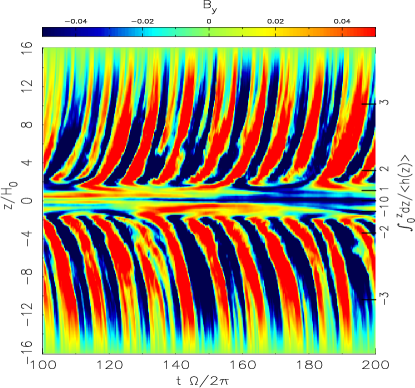
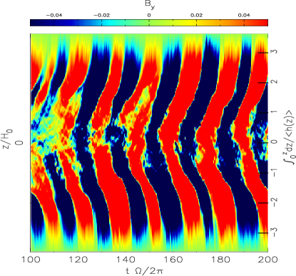
Figure 14.— Same as Figure 10 but for the toroidal magnetic fields.

The evolution of toroidal magnetic fields, $B_{y}$, is widely discussed in terms of “dynamo” activity in disks by MRI (Brandenburg et al., 1995; Nishikori et al., 2006; Shi et al., 2010). In Figure 14, we compare the $t-z$ diagrams of the cases with $\gamma=1.4$ (upper panel) and 1.0 (lower panel). The isothermal case (lower panel) exhibits usual quasi-periodic changing of the sign of $B_{y}$, as seen by previous works (e.g. Davis et al., 2010). The case with $\gamma=1.4$ also shows quasi-periodic oscillations of the $B_{y}$, but the period is shorter than that in the isothermal case and the amplitude (contrast between red and blue regions) is smaller. The tendency is similar for other large $\gamma(\geq 1.1)$ cases. This indicates that the toroidal magnetic fields change the sign before the magnetic fields are amplified to the level as strong as that obtained in the isothermal case. This is probably because in the large $\gamma$ case the magnetic fields are more subject to the gas motion because of the high $\beta$ condition (Figure 8).

The difference of the time-dependencies is consistent with the time evolutions of $\langle\alpha\rangle_{x,y,z}$ as shown in Figure 1. For larger $\gamma$, $\langle\alpha\rangle_{x,y,z}$ shows smaller fluctuations with time, because the dynamics are largely controlled by the gas pressures, which distribute more uniformly in a more time-steady manner, rather than by the magnetic fields, which intermittently pile up associated with channel flows.

Another interesting feature of the non-isothermal case with $\gamma=1.4$ is that the butterfly pattern triggered in the coronal regions is very vague in the midplane region. The left panel of Figure 9 also shows that the Poynting flux is negligibly small in this region. They imply that the miplane region seems to be protected from the magnetic perturbations in the coronal regions. The transition region which separates the cool midplane and the hot corona accompanies the large density difference to satisfy the pressure balance structure (Figure 6). This inevitably leads to the large jump of the Alfvén speed, $v_{{\rm A},z}$, across the transition region. Then, Alfvénic perturbations arising from magnetic tension suffer reflection and the downward Poynting flux from the coronal regions are mostly reflected back and cannot penetrate the transition regions to the midplane. Reflection of Alfvén waves is widely discussed on the sun because it is very efficient at the transition region between the cool chromosphere and the hot corona (e.g., Suzuki & Inutsuka, 2005; Matsumoto & Suzuki, 2012). A signature of reflected Alfvén waves is actually observed on the solar surface by the HINODE satellite (Fujimura & Tsuneta, 2009). These are quite similar to what we observe in the present simulations with relatively large $\gamma$.

4. Summary and Discussion

Using the 3D MHD simulations in the local stratified shearing boxes with weak net vertical magnetic fields, we have studied the formation of the hot coronae and the disk winds induced by the MRI turbulence in the accretion disks. Taking into account the effect of the cooling phenomenologically with the effective ratio of the specific heats, $\gamma$, we have inspected how the basic properties are affected by the cooling. Since the simulations are performed in the nondimensional form without any physical scale, the simulations are applicable to various objects. The amplifications of the magnetic fields are observed in all the simulation runs with different $\gamma$ from 1 to 5/3, which give the time- and box-averaged $\alpha\approx(1-3)\times 10^{-2}$, whereas we should take these values with cares because the numerical resolution is not sufficient in the midplane region.

The properties of the coronae and the disk winds are not so affected by the numerical resolution because the simulations well capture the MRI there, and we have found that the results are classified into the two regimes. In the small $\gamma(<1.03)$ regime, the temperatures in the surface regions are not high because the effect of the heating is weak owing to the small $\gamma$. The vertical outflows are directly driven by the Poynting flux associated with the amplified turbulent magnetic fields, they are more time-dependent, involved with the intermittent breakups of large-scale channel flows.

In the large $\gamma(\geq 1.1)$ regime, the hot coronae form by the dissipation of the magnetic energy and the temperatures are $\sim 50$ times of the initial values with the time-averaged peak temperature slowly increasing with $\gamma$. The vertical outflows are mainly driven by the gas pressure of the hot coronae. Because the spatial distribution of the gas pressure is more uniform than that of the magnetic energy, the disk winds stream out in a more time-steady manner than in the small $\gamma$ regime. The hot coronae are connected to the cool midplane through the sharp transition regions. Across the transition regions, both the sound and Alfvén speeds change abruptly because of the jumps of the temperature and the density. The transition regions work as the walls against wave activity. Sound-like waves are confined in the cool midplane region with giving the larger amplitudes of the density perturbations. The midplane region is also protected from the magnetic perturbations in the upper coronae.

Although the driving mechanisms and the time-dependencies of the vertical outflows are different for the small and large $\gamma$ regimes, the time-averaged nondimensional mass fluxes, $C_{\rm W}$, are similar each other. This is because in both the regimes the origin that drives the vertical outflows is the magnetic energy that is amplified by the MRI. The magnetic energy is gradually converted at the locations with $\rho\approx 10^{-2}-10^{-3}\rho_{\rm mid}$, directly to the kinetic energy of the disk winds in the small $\gamma$ regime, or firstly to the thermal energy of the hot coronae that is finally transferred to the disk winds in the large $\gamma$ regime. The location of the energy conversion, which is insensitive to $\gamma$, controls the final $C_{\rm W}$. We should cautiously note that the derived mass flux, $C_{\rm W}\approx 2\times 10^{-4}$, depends on the vertical box size (Suzuki et al., 2010; Fromang et al., 2013), although the comparisons of different cases with the same vertical box size make sense.

Our treatment of spatially uniform $\gamma$ is too much simplified. In reality, $\gamma$ should be non-uniform. Deeper regions near the midplane tend to be more optically thick, which gives larger $\gamma$, while in surface regions $\gamma$ is smaller. In more elaborated models with applications to specific objects, adequate cooling and heating processes should be included with radiative transfer (e.g., Hirose et al., 2006).

The authors thank Prof. Shu-ichiro Inutsuka for many fruitful discussion. The authors also appreciate constructive comments by an anonymous referee. This work was supported in part by Grants-in-Aid for Scientific Research from the MEXT of Japan, 22864006. Numerical simulations in this work were carried out with SR16000 at the Yukawa Institute Computer Facility and with the Cray XT4 and XC30 operated in CfCA, National Astrophysical Observatory of Japan.

References

- Bai & Stone (2013) Bai, X.-N., & Stone, J. M. 2013, ApJ, 767, 30
- Balbus & Hawley (1991) Balbus, S. A., & Hawley, J. F. 1991, ApJ, 376, 214
- Balbus & Hawley (1998) —. 1998, Reviews of Modern Physics, 70, 1
- Blandford & Payne (1982) Blandford, R. D., & Payne, D. G. 1982, MNRAS, 199, 883
- Bodo et al. (2012) Bodo, G., Cattaneo, F., Mignone, A., & Rossi, P. 2012, ApJ, 761, 116
- Brandenburg et al. (1995) Brandenburg, A., Nordlund, A., Stein, R. F., & Torkelsson, U. 1995, ApJ, 446, 741
- Chandrasekhar (1960) Chandrasekhar, S. 1960, Proceedings of the National Academy of Science, 46, 253
- Clarke (1996) Clarke, D. A. 1996, ApJ, 457, 291
- Coffey et al. (2004) Coffey, D., Bacciotti, F., Woitas, J., Ray, T. P., & Eislöffel, J. 2004, ApJ, 604, 758
- Davis et al. (2010) Davis, S. W., Stone, J. M., & Pessah, M. E. 2010, ApJ, 713, 52
- Flock et al. (2011) Flock, M., Dzyurkevich, N., Klahr, H., Turner, N. J., & Henning, T. 2011, ApJ, 735, 122
- Fromang et al. (2013) Fromang, S., Latter, H., Lesur, G., & Ogilvie, G. I. 2013, A&A, 552, A71
- Fujimura & Tsuneta (2009) Fujimura, D., & Tsuneta, S. 2009, ApJ, 702, 1443
- Goldreich & Lynden-Bell (1965) Goldreich, P., & Lynden-Bell, D. 1965, MNRAS, 130, 125
- Guan et al. (2009) Guan, X., Gammie, C. F., Simon, J. B., & Johnson, B. M. 2009, ApJ, 694, 1010
- Hawley et al. (1995) Hawley, J. F., Gammie, C. F., & Balbus, S. A. 1995, ApJ, 440, 742
- Hawley et al. (2011) Hawley, J. F., Guan, X., & Krolik, J. H. 2011, ApJ, 738, 84
- Hawley et al. (2013) Hawley, J. F., Richers, S. A., Guan, X., & Krolik, J. H. 2013, ApJ, 772, 102
- Hirose et al. (2006) Hirose, S., Krolik, J. H., & Stone, J. M. 2006, ApJ, 640, 901
- Hirose & Turner (2011) Hirose, S., & Turner, N. J. 2011, ApJ, 732, L30
- Lesur et al. (2013) Lesur, G., Ferreira, J., & Ogilvie, G. I. 2013, A&A, 550, A61
- Lynden-Bell & Pringle (1974) Lynden-Bell, D., & Pringle, J. E. 1974, MNRAS, 168, 603
- Machida et al. (2013) Machida, M., Nakamura, K. E., Kudoh, T., et al. 2013, ApJ, 764, 81
- Matsumoto & Tajima (1995) Matsumoto, R., & Tajima, T. 1995, ApJ, 445, 767
- Matsumoto & Suzuki (2012) Matsumoto, T., & Suzuki, T. K. 2012, ApJ, 749, 8
- Miller & Stone (2000) Miller, K. A., & Stone, J. M. 2000, ApJ, 534, 398
- Nishikori et al. (2006) Nishikori, H., Machida, M., & Matsumoto, R. 2006, ApJ, 641, 862
- Noble et al. (2010) Noble, S. C., Krolik, J. H., & Hawley, J. F. 2010, ApJ, 711, 959
- Ohashi et al. (1997) Ohashi, N., Hayashi, M., Ho, P. T. P., & Momose, M. 1997, ApJ, 475, 211
- Okuzumi & Hirose (2011) Okuzumi, S., & Hirose, S. 2011, ApJ, 742, 65
- Parker (1955) Parker, E. N. 1955, ApJ, 122, 293
- Parkin & Bicknell (2013a) Parkin, E. R., & Bicknell, G. V. 2013a, ApJ, 763, 99
- Parkin & Bicknell (2013b) —. 2013b, MNRAS
- Pudritz & Norman (1983) Pudritz, R. E., & Norman, C. A. 1983, ApJ, 274, 677
- Sai et al. (2013) Sai, K., Katoh, Y., Terada, N., & Ono, T. 2013, ApJ, 767, 165
- Sano et al. (1999) Sano, T., Inutsuka, S., & Miyama, S. M. 1999, in Astrophysics and Space Science Library, Vol. 240, Numerical Astrophysics, ed. S. M. Miyama, K. Tomisaka, & T. Hanawa, 383
- Sano et al. (2004) Sano, T., Inutsuka, S.-i., Turner, N. J., & Stone, J. M. 2004, ApJ, 605, 321
- Shakura & Sunyaev (1973) Shakura, N. I., & Sunyaev, R. A. 1973, A&A, 24, 337
- Shi et al. (2010) Shi, J., Krolik, J. H., & Hirose, S. 2010, ApJ, 708, 1716
- Simon et al. (2009) Simon, J. B., Hawley, J. F., & Beckwith, K. 2009, ApJ, 690, 974
- Stone et al. (1996) Stone, J. M., Hawley, J. F., Gammie, C. F., & Balbus, S. A. 1996, ApJ, 463, 656
- Suzuki & Inutsuka (2005) Suzuki, T. K., & Inutsuka, S.-i. 2005, ApJ, 632, L49
- Suzuki & Inutsuka (2006) —. 2006, Journal of Geophysical Research (Space Physics), 111, 6101
- Suzuki & Inutsuka (2009) —. 2009, ApJ, 691, L49
- Suzuki & Inutsuka (2013) —. 2013, submitted to ApJ
- Suzuki et al. (2010) Suzuki, T. K., Muto, T., & Inutsuka, S.-i. 2010, ApJ, 718, 1289
- Tombesi et al. (2010) Tombesi, F., Sambruna, R. M., Reeves, J. N., et al. 2010, ApJ, 719, 700
- Turner (2004) Turner, N. J. 2004, ApJ, 605, L45
- Velikhov (1959) Velikhov, E. P. 1959, Zh. Eksp. Teor. Fiz., 36, 1398