Feedback control of flow alignment in sheared liquid crystals

Abstract

Based on a continuum theory, we investigate the manipulation of the non-equilibrium behavior of a sheared liquid crystal via closed-loop feedback control. Our goal is to stabilize a specific dynamical state, that is, the stationary ”flow-alignment”, under conditions where the uncontrolled system displays oscillatory director dynamics with in-plane symmetry. To this end we employ time-delayed feedback control (TDFC), where the equation of motion for the $i$th component, $q_{i}(t)$, of the order parameter tensor is supplemented by a control term involving the difference $q_{i}(t)-q_{i}(t-\tau)$. In this diagonal scheme, $\tau$ is the delay time. We demonstrate that the TDFC method successfully stabilizes flow alignment for suitable values of the control strength, $K$, and $\tau$; these values are determined by solving an exact eigenvalue equation. Moreover, our results show that only small values of $K$ are needed when the system is sheared from an isotropic equilibrium state, contrary to the case where the equilibrium state is nematic.

I Introduction

Liquid crystals under shear can display a variety of non-equilibrium dynamical states determining the motion of the director of the (shear-induced or spontaneous) orientational ordering. The simplest of these states is the stationary ”flow-alignment” typically occurring at large shear rates and/or large values of the (particle geometry-related) coupling parameter $\lambda_{\mathrm{K}}$. However, the systems can also display various types of oscillatory motion, spatio-temporal symmetry breaking, and even chaotic behavior Rienäcker et al. (2002a, b); Grosso et al. (2003); Forest et al. (2004); Ripoll et al. (2008); Das et al. (2005). The discovery of this rich dynamical behavior has stimulated intense research both by theoretical methods (such as continuum approaches Hess (1975, 1976); Doi (1980, 1981); Olmsted and Goldbart (1992) and particle-based computer simulations Tao et al. (2005, 2009); Germano and Schmid (2005); Ripoll et al. (2008)) and by experiments (see, e.g., Bandyopadhyay et al. (2000); Lettinga et al. (2005)).

The nonlinear orientational dynamics also has direct implications for the rheological behavior of the system as reflected, e.g., by non-monotonic stress-strain curves (”constitutive relations”) Fielding (2007); Aradian and Cates (2005); Cates et al. (2002); Aradian and Cates (2006); Goddard et al. (2008); Klapp and Hess (2010); Heidenreich et al. (2009) and a non-Newtonian behavior of the viscosity. Understanding the dynamics is thus a prerequisite for the deliberate design of materials with specific rheological properties, which are tunable by parameters such as particle geometry, concentration (temperature) and external fields.

Beyond pure understanding, however, one may wish to stabilize a certain dynamic state with a well-defined associated rheology. A candidate for stabilization could be the stationary shear-alignment state. Indeed, it has been shown Hess and Kröger (2004); Klapp and Hess (2010) that the viscosity in such a state is particularly low (”shear-thinning”), in fact, lower than the viscosity of the corresponding unsheared system. In other words the stationary alignment of the liquid crystal molecule in the shear flow tends to lower frictional effects. This situation changes dramatically when the nematic director starts to oscillate Klapp and Hess (2010). Thus, shear-aligned systems may serve as particularly good lubricants.

In this paper we investigate the possibility to stabilize the flow-aligned state by a continuum approach for the orientational dynamics Hess (1975, 1976), combined with the method of time-delayed feedback control (TDFC). The relevant dynamical variable within the continuum approach is the second-rank alignment tensor ${\bf a}(t)$ carrying five independent components. In a previous, short study Strehober et al. (2012) we have already shown the TDFC to be successful if the dynamics of the full ${\bf a}(t)$ is simplified into that of a two-dimensional director characterizing uniaxial, shear-induced ordering within the shear plane. In the present paper we release this somewhat artificial restriction and investigate the full (in-plane) dynamics under TDFC. We focus on conditions where the uncontrolled system displays a wagging-like oscillatory motion within the shear plane. In this situation it seems tempting to consider only a reduced (three-dimensional system) involving only those components of the order parameter ${\bf a}$, which describe in-plane dynamics. However, as it was demonstrated in previous studies Rienäcker (2000); Rienäcker et al. (2002b), this reduction can predict a stable fixed point (the so-called log-rolling) which is actually unstable after inclusion of the remaining components of the order parameter. We thus consider the full five dimensional dynamical system to explore stability.
As in our earlier work Strehober et al. (2013), we did make some simplifying assumptions. First, we do not consider back-coupling of the orientational dynamics onto the flow. Rather we assume that the velocity field is imposed externally. Extensions of the theory incorporating such effects are proposed in a study of Lima and Rey de Andrade Lima and Rey (2004) as well as by Heidenreich et al. Heidenreich et al. (2009). Second we neglect the role of boundaries, which was discussed by Tsuji and Rey Tsuji and Rey (1997) as well as in Heidenreich et al. (2009). A third assumption is that we consider our sheared system being free of defects (for corresponding extensions see Rey and Denn (2002)).
Moreover, in the context of TDFC, we explore the interplay between the performance of the control scheme, on the one side, and the nature of the underlying equilibrium phase from which the liquid crystal is sheared, on the other side. TDFC is a closed-loop control method proposed 1992 by Pyragas Pyragas (1992), which allows one to stabilize periodic and steady states which would be unstable otherwise. In the meantime, TDFC has been applied to a broad variety of nonlinear systems including semiconductor nanostructures Baba et al. (2002); Unkelbach et al. (2003); Schlesner et al. (2003); Kehrt et al. (2009), lasers Dahms et al. (2008, 2010), excitable media Schlesner et al. (2006, 2008); Kyrychko et al. (2009), and neural systems Dahlem et al. (2008); Schöll et al. (2009); Panchuk et al. (2012) (see Schöll and Schuster (2008); Schöll (2009) for overviews). Within the Pyragas method, the equations of motion are supplemented by control terms built on the differences $q_{i}(t)-q_{i}(t-\tau)$ between the present and an earlier value of an appropriate system variable $q_{i}$. This type of control is noninvasive as the control forces vanish when the steady state (or a periodic state with period $T=n\tau$, with $n=1,2,3,\dots$) is reached. A general, analytic investigation of the application of TDFC to steady states has been given in Ref. Hövel and Schöll (2005).

The paper is organized as follows. We start in Sec. II with a review of the basic dynamical equations for the order parameter, $\bm{a}(t)$. In Sec. III.1 we summarize the dynamical behavior occurring in dependence of the shear rate and the coupling parameter for two temperatures (and correspondingly, different phases) of the underlying equilibrium system (for a full discussion based on a bifurcation analysis, see Ref. Strehober et al. (2013). For each reduced temperature $\theta$, we select a parameter set in which the uncontrolled system displays oscillatory director dynamics within the shear plane. The theoretical background of the TDFC method is introduced in Sec. III.2. Numerical results for the selected parameter sets are presented in Sec. IV. Finally, we give a conclusion and outlook.

II Background: Continuum theory of the orientational dynamics under shear

We employ a mesoscopic description of the system, where the relevant dynamic variable is the orientational order parameter averaged over some volume in space. In a sheared liquid crystal, this order parameter corresponds to the time-dependent, 2nd-rank alignment tensor ${\bf a}=\sqrt{15/2}\langle\mbox{ $\hskip 1.00006pt\stackrel{{\scriptstyle\rule{0.3pt}{0.8288pt}\overline{\hphantom{\mbox{$\displaystyle{\bf u}{\bf u}$}}}\rule{0.3pt}{0.8288pt}}}{{{\bf u}{\bf u}}}\hskip 1.99997pt$ }\rangle$, where ${\bf u}$ describes the orientation of the molecular axis and $\hskip 1.00006pt\stackrel{{\scriptstyle\rule{0.3pt}{0.8288pt}\overline{\hphantom{\mbox{$\displaystyle\ldots$}}}\rule{0.3pt}{0.8288pt}}}{{\ldots}}\hskip 1.99997pt$ indicates the symmetric traceless part of a tensor. The average $\langle\ldots\rangle$ is defined as (see Ref. Strehober et al. (2013))

$$\langle\ldots\rangle=\int_{S^{2}}{\mathrm{d}}^{2}\bm{u}\,\ldots\,\rho^{\mathrm{or}}(\bm{u},\bm{r},t),$$ (1)

involving the orientational distribution function $\rho^{\mathrm{o}r}(\bm{u},\bm{r},t)$ Sonnet et al. (1995). The integral in Eq. (1) is performed over the unit sphere. The orientational distribution is defined as $\rho^{\mathrm{or}}(\bm{u},\bm{r},t)=N^{-1}\langle\sum_{i=1}^{N}\delta(\bm{u}-\bm{u}_{i}(t))\rangle_{\mathrm{ens}}$, where $\bm{u}_{i}$ is the microscopic orientation of particle $i$ ($i=1,\ldots,N$), and $\langle\ldots\rangle_{\mathrm{ens}}$ is an ensemble average in a small volume $dV$ around the space point $\bm{r}$ at time $t$.

In the isotropic equilibrium state, all components of ${\bf a}$ are zero, whereas nematic ordering (which may be uniaxial or biaxial in character) is characterized by one or several components of ${\bf a}$ being non-zero.

Switching on an external shear flow characterized by a velocity field ${\bf v}$, the alignment tensor becomes a time-dependent quantity. Its equation of motion can be derived from a generalized Fokker-Planck equation Hess (1976); Doi (1980, 1981) or, alternatively, from irreversible thermodynamics Hess (1975), yielding for a homogeneous system (in dimensionless form) Grandner et al. (2007a)

$$\frac{d{\bf a}}{dt}=2\mbox{ $\hskip 1.00006pt\stackrel{{\scriptstyle\rule{0.3pt}{0.8288pt}\overline{\hphantom{\mbox{$\displaystyle{\bm{\Omega}}\cdot{\bf a}$}}}\rule{0.3pt}{0.8288pt}}}{{{\bm{\Omega}}\cdot{\bf a}}}\hskip 1.99997pt$ }+2\sigma\,\mbox{ $\hskip 1.00006pt\stackrel{{\scriptstyle\rule{0.3pt}{0.8288pt}\overline{\hphantom{\mbox{$\displaystyle{\bm{\Gamma}}\cdot{\bf a}$}}}\rule{0.3pt}{0.8288pt}}}{{{\bm{\Gamma}}\cdot{\bf a}}}\hskip 1.99997pt$ }-{\Phi}^{\prime}(\bm{a})+\sqrt{\frac{3}{2}}\lambda_{\mathrm{K}}\,{\bm{\Gamma}}.$$ (2)

In Eq. (2), ${\bm{\Gamma}}=\left((\nabla{\bf v})^{T}+\nabla{\bf v}\right)/2$ is the strain rate tensor (with the superscript ”T” denoting the transpose of tensor $\nabla{\bf v}$) and ${\bm{\Omega}}=\left((\nabla{\bf v})^{T}-\nabla{\bf v}\right)/2$ is the vorticity. The symbol $\hskip 1.00006pt\stackrel{{\scriptstyle\rule{0.3pt}{0.8288pt}\overline{\hphantom{\mbox{$\displaystyle\bf{x}$}}}\rule{0.3pt}{0.8288pt}}}{{\bf{x}}}\hskip 1.99997pt$ indicates the symmetric traceless part of a tensor $\bf{x}$, i.e. $\mbox{ $\hskip 1.00006pt\stackrel{{\scriptstyle\rule{0.3pt}{0.8288pt}\overline{\hphantom{\mbox{$\displaystyle{\bf x}$}}}\rule{0.3pt}{0.8288pt}}}{{{\bf x}}}\hskip 1.99997pt$ }=1/2({\bf x}+{\bf x}^{T})-1/3Tr({\bf x})$. In the present work we consider a planar Couette flow characterized by ${\bf v}=\dot{\gamma}y{\bf e}_{\mathrm{x}}$, with $\dot{\gamma}$ being the shear rate and ${\bf e}_{\mathrm{x}}$ being a unit vector. This yields ${\bm{\Gamma}}=\dot{\gamma}\mbox{ $\hskip 1.00006pt\stackrel{{\scriptstyle\rule{0.3pt}{0.8288pt}\overline{\hphantom{\mbox{$\displaystyle{\bf e}_{\mathrm{x}}{\bf e}_{\mathrm{y}}$}}}\rule{0.3pt}{0.8288pt}}}{{{\bf e}_{\mathrm{x}}{\bf e}_{\mathrm{y}}}}\hskip 1.99997pt$ }$ and ${\bm{\Omega}}=(\dot{\gamma}/2)\left({\bf e}_{\mathrm{x}}{\bf e}_{\mathrm{y}}-{\bf e}_{\mathrm{y}}{\bf e}_{\mathrm{x}}\right)$, respectively. The (dimensionless) parameter $\lambda_{\mathrm{K}}$ is the so-called ”tumbling” parameter, which measures the coupling strength between alignment and strain. This parameter is related to the shape (i.e., the aspect ratio) of the particles Hess (1976). The relaxation parameter $\sigma$ plays only a minor role, and following previous works Hess and Kröger (2005); Rienäcker et al. (2002a); Grandner et al. (2007b, c); Strehober et al. (2013), we set $\sigma=0$. Finally, the (tensorial) quantity ${\Phi}^{\prime}(\bm{a})$ appearing in Eq. (2) corresponds to the derivative of the free energy with respect to the (non-conserved) order parameter, i.e., ${\Phi}^{\prime}(\bm{a})=\partial\Phi/\partial{\bf a}$. We employ the (dimensionless) Landau-de Gennes (LG) expression for the free energy de Gennes and Prost (1993) given by

$$\Phi=\frac{\theta}{2}{\bf a}:{\bf a}-\sqrt{6}\left({\bf a}\cdot{\bf a}\right):{\bf a}+\frac{1}{2}\left({\bf a}:{\bf a}\right)^{2},$$ (3)

where the notation ”:” stands for the trace over the product of two tensors, and ”$\cdot$” indicates conventional matrix multiplication. In Eq. (3), $\theta$ plays the role of an effective, dimensionless temperature, which is the tuning parameter for the isotropic-nematic transition in thermotropic liquid-crystal-systems. A first order isotropic-nematic transition occurs at $\theta=1$. For temperatures $\theta>1$ ($\theta<1$) the isotropic (nematic) phase is stable, i.e., it corresponds to the lowest minimum of the free energy. Upon “cooling down” from high temperatures, the nematic state appears as a metastable phase already at $\theta=9/8$. Crossing the phase transition (at $\theta=1$), the isotropic phase remains as a metastable phase down to $\theta=0$, below which it becomes unstable. We note that this general scenario applies not only to thermotropic liquid crystals (where $\theta$ is related to a true temperature), but also to lyotropic liquid crystals and suspensions of colloidal rods. In these cases, the isotropic-nematic transition is triggered by the concentration, and $\theta$ has to be defined accordingly Strehober et al. (2013), otherwise the approach remains the same.

Equation (2) is most conveniently solved by expanding $\bm{a}$ and the other tensors appearing on the right side into a tensorial basis set (see, e.g., Rienäcker et al. (2002b)), e.g., $\bm{a}=\sum_{l=0}^{4}a_{l}{\bf T}^{l}$, where $a_{l}$ are the (five) independent components of ${\bf a}$, and the (orthonormal) tensors ${\bf T}^{l}$ involve linear combinations of the unit vectors ${\bf e}_{\mathrm{x}}$, ${\bf e}_{\mathrm{y}}$, and ${\bf e}_{\mathrm{z}}$ (for explicit expressions, see e.g. in Ref. Rienäcker et al. (2002b)). One then obtains the five-dimensional dynamical system

$$\dot{\bm{q}} =\bm{F},$$ (4)

where the vector $\bm{q}=(a_{0},a_{1},a_{2},a_{3},a_{4})$, and the components of the vector $\bm{F}$ are given by

$${F}_{0}= -\phi_{0}$$

$${F}_{1}= -\phi_{1}+\dot{{\gamma}}a_{2}$$

$${F}_{2}= -\phi_{2}-\dot{{\gamma}}a_{1}+{\frac{1}{2}}{\sqrt{3}}{\lambda}_{K}\dot{{\gamma}}$$

$${F}_{3}= -\phi_{3}+{\frac{1}{2}}\dot{{\gamma}}a_{4}$$

$${F}_{4}= -\phi_{4}-{\frac{1}{2}}\dot{{\gamma}}a_{3}.$$ (5)

In Eqs. (5), the quantities $\phi_{l}$ ($l=0,\ldots,4$) represent the components of the vector ${\bm{\Phi}}$ (that consist of the projections of ${\Phi}^{\prime}(\bm{a})$ on the tensor basis). These quantities are nonlinear functions of the $a_{l}$; explicit expressions are given in the appendix.

III Feedback control

III.1 Choosing candidate states

The dynamical behavior emerging from the mesoscopic equations of motion (4) has been studied in detail for a variety of temperatures $\theta$ (determining the behavior of the unsheared system) and a broad range of shear rates $\dot{\gamma}$ and shear coupling parameters $\lambda_{\mathrm{K}}$ Strehober et al. (2013); Hess and Kröger (2005); Heidenreich (2008); Rienäcker (2000); Rienäcker et al. (2002a, b). In particular in Ref. Strehober et al. (2013), we have investigated systems at different temperatures via a numerical bifurcation analysis (for numerical details see Appendix of Strehober et al. (2013)). Special attention has been devoted to systems sheared from the stable or metastable nematic equilibrium phase ($\theta\leq 9/8$). An exemplary dynamical state diagram for the case $\theta=0$ is shown in Fig. 1 (data taken from Ref. Strehober et al. (2013) and the diagram is consistent with earlier works, i.e. Rienäcker et al. (2002a, b); Rienäcker (2000)).

Figure 1: (Color online) Dynamical state diagram in the plane spanned by the tumbling parameter $\lambda_{\mathrm{K}}$ and the (dimensionless) shear rate $\dot{\gamma}$ for a nematic system ($\theta=0$). The lines were obtained via a codimension-2 bifurcation analysis as described in Ref. Strehober et al. (2013). The nearly vertical line represents a supercritical Hopf bifurcation line (H). On the right side of the H line we find flow alignment (A), corresponding to a stable fixed point. This is indicated by the notation (1s,0u), where ”1s” and ”0u” means one stable (s) and no unstable (u) fixed point, respectively. Upon crossing the H line towards lower values of $\lambda_{\mathrm{K}}$, oscillatory in-plane states [wagging (W) and tumbling (T)] become stable. As indicated by the notations (0s,3u) [and (0s,1u)] there is no stable fixed point in this area, but three [one] unstable ones. The cross marks the parameter set $\bm{\beta}_{\mathrm{I}}=(\lambda_{\mathrm{K}}=1.0,\dot{\gamma}=5.0,\theta=0)$ where we apply feedback control. The shaded areas appearing at low $\dot{\gamma}$ correspond to oscillatory states with out-of-plane symmetry. The lines labeled LP1 and LP2 are limit point lines (saddle-node bifurcation lines).

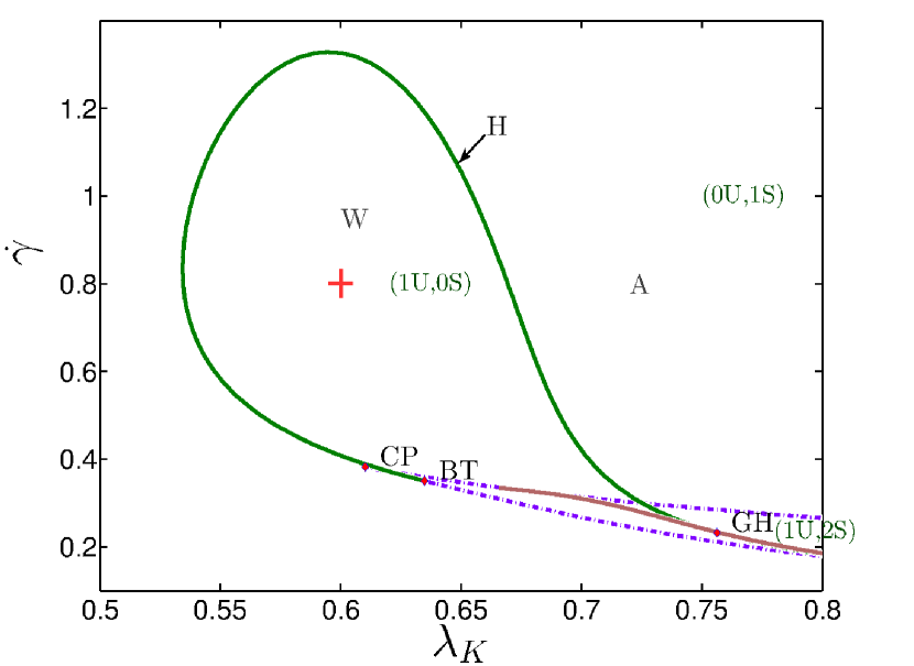
Figure 2: (Color online) Dynamical state diagram at $\theta=1.20$, where the unsheared system is isotropic. The lines are obtained via a codimension-2 bifurcation analysis as described in Ref. Strehober et al. (2013). With the bifurcation analysis we also detect special points like cusp point (CP), Bogdanov-Takens point (BT) and generalized Hopf point (GH). The solid line (shaped like an oval) represents a supercritical H bifurcation line, within which the system is in an oscillatory (W) state. The cross marks the parameter set $\bm{\beta}_{\mathrm{II}}=(\lambda_{K}=0.6,\dot{\gamma}=0.8,\theta=1.20)$ selected as a second candidate for feedback control. Outside this W regime (characterized by one unstable fixed point), the system is in a stationary, flow-aligned state (A). The dashed lines appearing in the right, lower corner of the diagram are limit point lines (LP) (saddle-node bifurcation lines). Between the LP curves one finds areas of bistability between paranematic and nematic states (for details on that see Ref. Strehober et al. (2013)). The notation regarding the fixed points is as in Fig. 1.

For large values of the shear rate ($\dot{\gamma}\gtrsim 4.5$, i.e., above the semicircle line in Fig. 1) the stable dynamical states have in-plane symmetry. In this case the main director is restricted to directions within the shear plane (i.e., the $x$-$y$-plane), implying that the components $a_{3}=a_{4}=0$. At large values of the coupling parameter $\lambda_{\mathrm{K}}$, this in-plane state is stationary in character, reflecting that the nematic director is ”frozen” and encloses a fixed angle with the direction of the shear flow. This is the so-called ”flow alignment” state, which we label by A. Mathematically, the A state corresponds to a stable fixed point of the dynamics. Decreasing the coupling parameter $\lambda_{\mathrm{K}}$ (at fixed, large $\dot{\gamma}$), one encounters a supercritical Hopf bifurcation Strehober et al. (2013) and the system displays oscillatory states with in-plane symmetry. These are the so-called wagging (W) occurring at intermediate values of $\lambda_{\mathrm{K}}$, and the tumbling (T) state at low $\lambda_{\mathrm{K}}$, Both T and W are characterized by the presence of stable limit cycles, and, correspondingly, unstable fixed points (for a more detailed discussion, see Sec. IV). In the W state the angle between the nematic director and the flow direction oscillates periodically between a minimal and a maximal value, whereas in the T state, the director performs full, in-plane rotations. We stress, however, that there is no fundamental difference between W and T motion in the sense that these states are not separated by a bifurcation Strehober et al. (2013).

At lower shear rates, additional dynamical states appear which are characterized by non-zero values of all five components of the order parameter. Physically, this means that the main director performs oscillations not only within the shear plane, but also out of this plane. Typical representatives are the ”kayaking wagging” (KW) and ”kayaking tumbling” (KT) states first observed in Ref. Larson and Öttinger (1991). In Fig. 1, such out-of-plane solutions occur in the shaded regions. We have also indicated regions of bistability and complex chaotic behavior (for a more detailed discussion, see Refs. Strehober et al. (2013); Rienäcker (2000); Rienäcker et al. (2002a, b)).

The main goal of the present paper is to explore the stabilization of the fixed point corresponding to flow alignment within a parameter range where the system is in an in-plane oscillatory state (i.e., W or T). The specific position in parameter space is indicated by the cross in Fig. 1, corresponding to the parameter set $\bm{\beta}_{\mathrm{I}}:=(\lambda_{K}=1.0,\dot{\gamma}=5.0,\theta=0)$.

Our reasoning to focus on in-plane situations is twofold: First, the absence of stable out-of-plane solutions allows us to focus on only three components of the order parameter tensor, that is, $a_{0}$, $a_{1}$ and $a_{2}$. Second, it has been shown Strehober et al. (2013) that the out-of-plane states do not arise via a Hopf bifurcation. Thus, there is no ”natural” unstable fixed point which one could try to stabilize via TDFC.

In addition to a nematic system, we also consider in our study a system which is isotropic in the absence of shear ($\theta=1.20$). A corresponding state diagram is shown in Fig. 2. At large coupling parameters ($\lambda_{\mathrm{K}}\gtrsim 0.75$), the shear flow induces first ($\dot{\gamma}\lesssim 0.2$) a ”paranematic” ordering characterized by very small values of the order parameters. Increasing $\dot{\gamma}$ the systems then transforms via a first-order transition into a flow-aligned state (A). Interestingly, however, the system can also display an in-plane oscillatory state, that is, wagging (W). This behavior is rather surprising in view of the isotropic nature of the underlying equilibrium state and was detected only recently Strehober et al. (2013). As seen from Fig. 2, the wagging occurs in a parameter island located at lower values of $\lambda_{\mathrm{K}}$. The major part of the boundaries of this island represent Hopf bifurcations. We select a parameter point within this wagging island as a second candidate for feedback control. Specifically, $\bm{\beta}_{\mathrm{II}}:=(\lambda_{K}=0.6,\dot{\gamma}=0.8,\theta=1.20)$.

Having identified suitable parameter sets ($\bm{\beta}_{\mathrm{I}},\bm{\beta}_{\mathrm{II}}$) to apply feedback control of steady states, we now turn to a detailed discussion of (i) the stability of the corresponding steady states, and (ii) their behavior under TDFC with diagonal control scheme. The corresponding methods are outlined in the subsequent Sec. III.2. In Sec. IV, we will present the numerical results.

As already remarked in the introduction, we perform the stability analysis described below with the full, five-dimensional system (see also discussion in Sec. IV.1). In this way we avoid difficulties arising if one considers the three-component system alone.

III.2 Time-delayed feedback control

As a starting point for feedback control, we first need to determine the steady states (fixed points) $\bm{q}^{\star}=(a_{0}^{\star},a_{1}^{\star},a_{2}^{\star},a_{3}^{\star},a_{4}^{\star})$ of the dynamical system [see Eq. (4)] corresponding to the two parameter sets $\bm{\beta}_{\mathrm{I}}$, $\bm{\beta}_{\mathrm{II}}$. The fixed points fulfill the condition $\dot{\bm{q}^{\star}}=0$. We have solved these equations numerically.

For each fixed point, its linear stability can be checked by considering the $5\times 5$ Jacobian ${\bf J}$ of the dynamical system. The elements $J_{ij}=\partial F_{i}/\partial q_{j}$ of ${\bf J}$ are given in the appendix A. Small perturbations $\delta{\bf q}(t)$ away from the steady state evolve with time as $\dot{\delta{\bf q}}(t)={\bf J}\delta{\bf q}(t)$. This linear equation can be solved with the ansatz $\delta{\bf q}(t)={\bf A}\exp[\nu t]$ (with ${\bf A}$ containing the real amplitudes of the perturbation), yielding the eigenvalue equation

$$\nu\delta{\bf q}={\bf J}\delta{\bf q}.$$ (6)

The eigenvalues can then be calculated from the characteristic equation $\mathrm{det}\left({\bf J}-\nu{\bf I}\right)=0$ (where ${\bf I}$ is the unity matrix). Stability of the fixed point $\bm{q}^{\star}=(a_{0}^{\star},a_{1}^{\star},a_{2}^{\star},a_{3}^{\star},a_{4}^{\star})$ requires that all eigenvalues of $\bm{J}$ evaluated at this fixed point have negative real parts, implying that perturbations die off with time.

We now aim to stabilize the unstable fixed point ${\bf q}^{\star}$ corresponding to flow alignment within the range, where the system ends up in wagging motion. To this end, we use the TDFC method Pyragas (1992). Following earlier work Hövel and Schöll (2005), we employ a diagonal control scheme, where the control force acting on the $i$th component (with $i=0,1,2,3,4$) involves only the same component. Explicitly,

$$\dot{q_{i}}=F_{i}({\bf q},\bm{\beta})-K\left(q_{i}(t)-q_{i}(t-\tau)\right)$$ (7)

where $K$ measures the strength of control and $\tau$ is the delay time. Note that the feedback terms in Eq. (7) vanish when the fixed point is fully stabilized, that is, if ${\bf q}^{\star}(t-\tau)={\bf q}^{*}(t)$. The impact of the control on the phase portrait, for the two different parameter sets ($\bm{\beta}_{\mathrm{A}}$, $\bm{\beta}_{\mathrm{II}}$), is shown in Sec. IV.

To get a better insight into the role of the feedback control, it is instructive to perform a (linear) stability analysis of the delayed differential equations given in (7) Hövel and Schöll (2005). In analogy to the procedure discussed before [see Eq. (20 below)], we consider a small displacement from the fixed point, $\delta{\bf q}(t)$. To linear order, the dynamics of this displacement follows from Eq. (7) as

$$\dot{\delta{\bf q}}=\left({\bf J}-K{\bf I}\right)\delta{\bf q}(t)+K\delta{\bf q}(t-\tau).$$ (8)

This equation can be solved with the exponential ansatz $\delta{\bf q}(t)={\bf B}\exp[\mu t]$, where ${\bf B}$ contains the amplitudes of the displacement, and $\mu$ is a complex number. Inserting this ansatz into Eq. (8) one obtains the eigenvalue equation

$$\left(\mu+K\left(1-\exp[-\mu\tau]\right)\right)\delta{\bf q}={\bf J}\delta{\bf q}.$$ (9)

The corresponding characteristic equation yielding the eigenvalues $\mu$ is given by

$$\mathrm{det}\left({\bf J}-\left(\mu+K\left(1-\exp[-\mu\tau]\right)\right){\bf I}\right)=0.$$ (10)

However, an even simpler way to calculate the eigenvalues $\mu$ is based on the following notion: Equation (9) has exactly the same form as the corresponding equation for the uncontrolled case, Eq. (6). In other words, the linear operator ${\bf J}$ has the same set of eigenfunctions $\delta{\bf q}$ in both, the uncontrolled and the controlled case. This notion implies that if the eigenvalues $\nu$ of the uncontrolled system are known, then the eigenvalues $\mu$ of the controlled system can be calculated from

$$\mu+K\left(1-\exp[-\mu\tau]\right)=\nu$$ (11)

We also stress that Eq. (11) is equivalent to the eigenvalue equation derived in Ref. Hövel and Schöll (2005). In that paper, the (diagonal) feedback control of unstable steady states in a two-dimensional dynamical system was studied from a general perspective, that is, without reference to a particular physical system. In particular, it was shown that Eq. (11) can be solved analytically by using the Lambert function ${\cal W}$ Corless et al. (1996). The same strategy can be used in the present, five-dimensional case, because we are using the same, diagonal control scheme. To see this, we rearrange Eq. (11) into

$$\left(\mu+K-\nu\right)\tau=K\tau\exp[-\mu\tau].$$ (12)

Setting $z=\left(\mu+K-\nu\right)\tau$ and multiplying both sides of Eq. (12) with $\exp[z]$ we have

$$z\exp[z]=K\tau\exp[\left(K-\nu\right)\tau]\equiv g.$$ (13)

We can solve this equation with respect to $z$ by using that $z={\cal W}(z\exp[z])={\cal W}(g)$. After re-substituting (i.e., $\mu\tau=z-(K-\nu)\tau$) we finally obtain the explicit formula

$$\mu\tau={\cal W}\left(K\tau\exp[-\nu\tau+K\tau]\right)+\nu\tau-K\tau.$$ (14)

We have calculated the eigenvalues both, numerically [from Eq. (10)] and analytically [from Eq. (14)] for a range of control parameters $K$, $\tau$, at the two parameter sets $\bm{\beta}_{\mathrm{I}}$ and $\bm{\beta}_{\mathrm{II}}$ (see Figs. 1 and 2, respectively). Notice that the TDFC scheme, which is based on the coupling of a dynamical variable to its own history [see Eq. (7)], creates an infinite number of eigenvalues and corresponding eigenmodes Hövel and Schöll (2005).

IV Results

IV.1 Fixed point stabilization in the nematic phase

We start by determining the (unstable) fixed points at the parameter set ${\bm{\beta}}_{\mathrm{I}}$ (see Fig. 1). Since we are in the regime of in-plane dynamic states ($a_{3}=a_{4}=0$) we can visualize the nullclines of the system, i.e. the geometrical shapes where $\dot{a}_{i}=0$, as two-dimensional surfaces in the three-dimensional space spanned by $(a_{0},a_{1},a_{2})$. These surfaces are shown in Fig. 3.

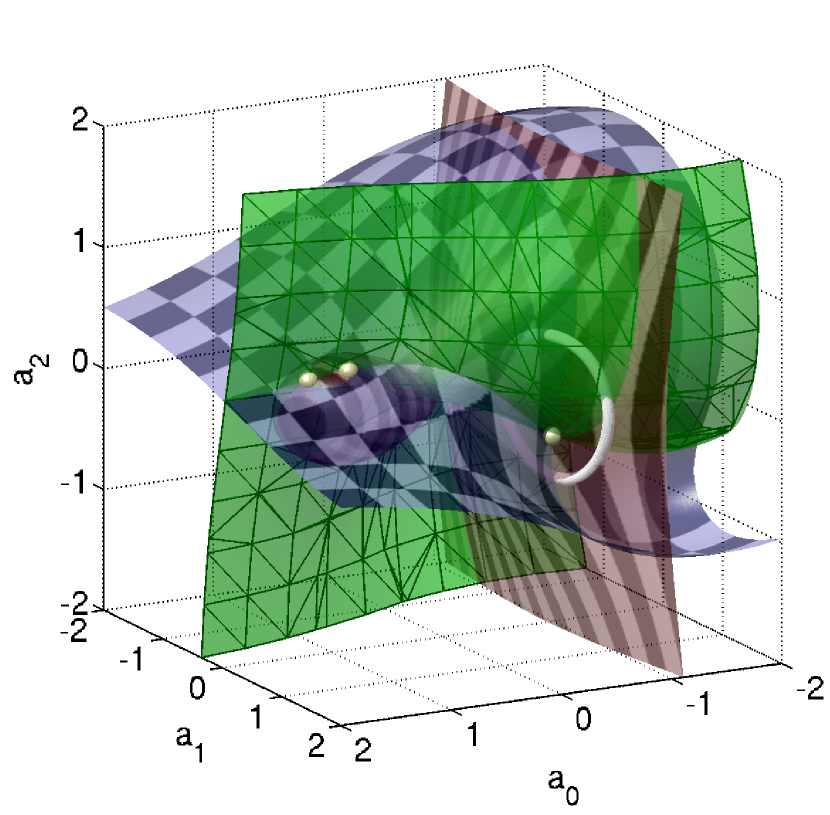
Figure 3: (Color online) Nullclines corresponding to the dynamical variables $a_{0}$, $a_{1}$, $a_{2}$. The parameters are fixed to the set ${\bm{\beta}}_{\mathrm{I}}$ located within the in-plane W regime (see Fig. 1). The striped, unichrome, and checkerboard patterned surface are obtained from setting $\dot{a_{0}}=0$, $\dot{a_{1}}=0$, and $\dot{a_{2}}=0$, respectively (the components $a_{3}$ and $a_{4}$ vanish at ${\bm{\beta}}_{\mathrm{I}}$). The small spheres indicate the intersections of all nullclines and thus depict the (unstable) fixed points of the system, $\bm{q}^{\star}_{1}=(1.30034,0.139206,0.318084,0,0)$, $\bm{q}^{\star}_{2}=(-0.563386,0.807425,-0.217522,0,0)$, and $\bm{q}^{\star}_{3}=(0.98609,0.232099,0.38358,0,0)$. The white cycle corresponds to the stable limit cycle emerging around $\bm{q}^{\star}_{2}$.

The fixed points of the system are located where all of the three nullclines intersect. As seen from Fig. 3, there are three fixed points (indicated by small spheres). An analysis of the corresponding Jacobian shows that all of these fixed points are unstable (i.e., at least one eigenvalue has a positive real part), as expected in the wagging regime. We remark in this context that the fixed point $\bm{q}^{\star}_{1}$ would actually be stable if we had restricted ourselves to the analysis of the 3-dimensional system ($a_{0},a_{1},a_{2}$). Indeed, in this case, all three eigenvalues related to $\bm{q}^{\star}_{1}$ have negative real parts. The corresponding ”log-rolling” state has been analyzed in Ref. Rienäcker et al. (2002b). In the full, five-dimensional analysis, however, this fixed point becomes unstable since the nematic director can ”escape” in further directions. The other fixed points, $\bm{q}^{\star}_{2}$ and $\bm{q}^{\star}_{3}$, are unstable in both the three- and the five-component dynamical system.

Also indicated in Fig. 3 is the (stable) limit cycle emerging around the fixed point $\bm{q}^{\star}_{2}$. This limit cycle corresponds to undamped oscillations of the order parameters as functions of time. The corresponding period is close to that predicted by linear stability analysis, $T_{0}=2\pi/|\mathrm{Im}(\nu)|$, where $\nu$ is one member of the (complex conjugate) pair of eigenvalues at $\bm{q}^{\star}_{2}$ that have a positive real part (numerically, we find $\nu\approx 0.49+\mathrm{i}4.61$, yielding $T_{0}\approx 1.36$). The dynamical evolution of an unstable configuration of dynamical variables towards the limit cycle is illustrated in Fig. 4 a).

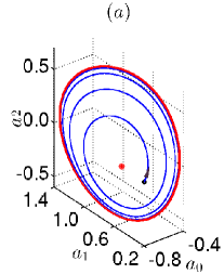
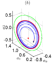
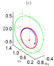
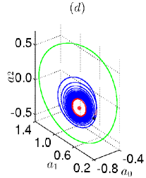
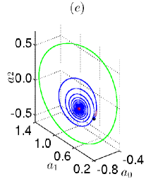
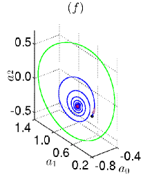
Figure 4: (Color online) Phase portraits of the dynamical variables $a_{i}$ ($i=0,1,2$). Parameters are fixed to the set ${\bm{\beta}}_{\mathrm{I}}$ located within the in-plane W regime (see Fig. 1). The central small (red) dot marks the (unstable) fixed point. (a) Uncontrolled system ($K=0$) with initial condition $a_{0}^{\mathrm{init}}=-0.57$, $a_{1}^{\mathrm{init}}=0.5$, $a_{2}^{\mathrm{init}}=-0.22$. The initial condition is indicated with a black diamond. (b)-(f) Systems under time-delayed feedback control [see Eq. (7)] with the control strength (b) $K=0.1$, (c) $0.2$, (d) $0.3$, (e) $0.4$, and (f) $0.5$, respectively, and delay time $\tau=0.5$. In all cases (b)-(f), the control starts at $t=0$, assuming that $a_{i}(t)=a_{i}^{\mathrm{init}}$ in the interval $[-\tau,0]$. In (a)-(d) the blue (dark) trajectories approach stable limit cycles, which are plotted as red (thick dark) cycles. In (b)-(f) the limit cycle of the uncontrolled system (a) is replotted for reference as green (light) cycle. For (e),(f) the trajectories end in the fixed point.

We now apply the TDFC scheme described in Sec. III.2. To illustrate the impact on the phase portraits, we show in Figs. 4 b)-f) exemplary results for a fixed delay time, $\tau=0.5$, and different values of the control strength, $K$. All calculations have been started with the same initial values for the order parameters, $a_{0}$, $a_{1}$, $a_{2}$, and the same history regarding the onset of control. Inspecting Figs. 4 it is seen that for $K\leq 0.3$, the feedback control reduces the diameter of the limit cycle but the dynamics remains oscillatory at long times [see parts (b)-(d)]. However, for $K=0.4$ and $K=0.5$, the initially oscillatory motion becomes more and more damped out with time, and the final state is the fixed point $\bm{q}^{\star}_{2}$. Physically, this means that the director freezes along an in-plane direction, corresponding to flow alignment. Thus, the control scheme has been successful.

A more systematic way to analyze the stability of the fixed point $\bm{q}^{\star}_{2}$ under feedback control is to monitor the complex eigenvalues $\mu$ [see Eq. (9)]. Specifically, we consider the largest real part of $\mu$. Indeed, due to the transcendental character of Eq. (11), the spectrum of eigenvalues of the controlled system is infinite due to the infinite number of branches of the Lambert ${\cal W}$ function (multileaf structure). Stabilization (within the linear approximation) of the fixed point then means that $\mathrm{max}\left(\mathrm{Re}\left(\mu\right)\right)$ is negative at the values of $K$ and $\tau$ considered.

To get a first insight into the ranges of control parameters, where TDFC works, we plot in Fig. 5 the quantity $\mathrm{max}\left(\mathrm{Re}\left(\mu\right)\right)$ as a function of $\tau$ for different values of the control strength $K$.

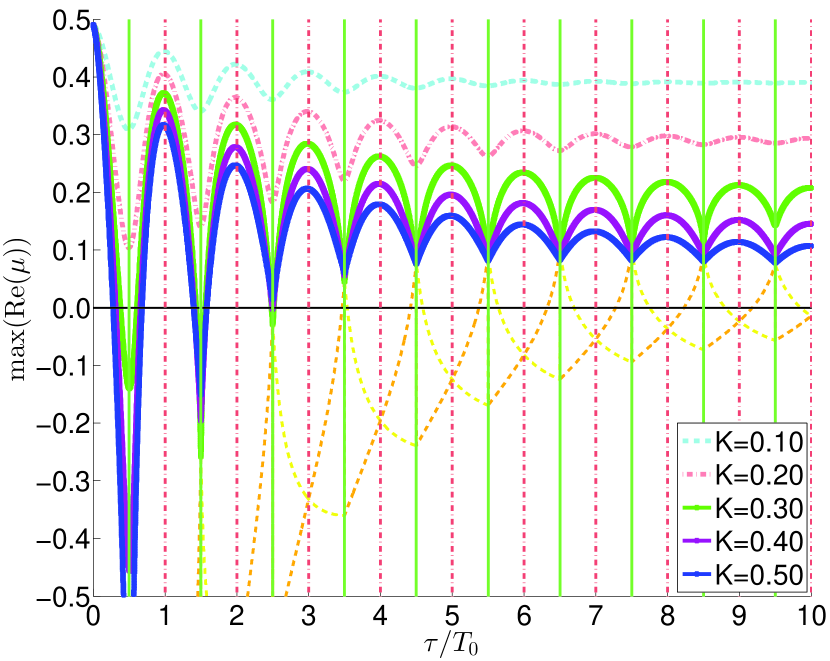
Figure 5: (Color online) Largest real part of the complex eigenvalues $\mu$ vs $\tau$ for different values of $K$. The dot-dashed vertical lines correspond to multiples of $T_{0}=2\pi/|\mathrm{Im}(\nu)|$ ($T_{0}\approx 1.36$), where $\nu$ is the eigenvalue of the uncontrolled system at the fixed point $\bm{q}^{\star}_{2}$ (see Fig. 3). The solid vertical lines are shifted relative to the dashed lines by $T_{0}/2$. The dashed lines in the lower part indicate some lower branches of eigenvalues for $K=0.30$. The other parameters are fixed to the set ${\bm{\beta}}_{\mathrm{I}}$ located within the in-plane W regime (see Fig. 1).

All curves start at the value of the real part corresponding to $\tau=0$ where the control terms in Eq. (7) vanish. The positive value indicates the instability of the steady state. Upon increase of the delay time from zero, the largest real parts corresponding to different $K$ first decrease up to a certain delay time, and display subsequently an oscillatory behavior. However, for the cases $K=0.1$ and $K=0.2$, the largest real part remains positive. Only for $K\geq 0.3$ there exist values of $\tau$ where the largest real parts become negative, indicating that the control is successful.

Following the analysis in Ref. Hövel and Schöll (2005), it is possible to analytically determine the minimum value of $K$ required to control the system at specific values of $\tau$. The boundary of stability is determined by the condition $\mathrm{Re}(\mu)=0$, or equivalently, $\mu=i\Omega$ (with $\Omega$ being real). Inserting this into Eq. (11) we find

$$\mathrm{Re}(\nu) = K\left(1-\cos\Omega\tau\right)$$

$$\mathrm{Im}(\nu) = \Omega+K\sin\Omega\tau.$$ (15)

From the first equation of Eq. (IV.1) it follows that at the boundary of stability, $K$ varies between $\mathrm{Re}(\nu)/2$ and $\infty$ (since $\cos\Omega\tau$ is bounded between $-1$ and $1$). Thus, the minimal value of $K$ is given by

$$K_{\mathrm{min}}=\mathrm{Re}(\nu)/2$$ (16)

corresponding to $\cos\Omega\tau=-1$. The fixed point $\bm{q}^{\star}_{2}$ considered here is characterized by $\mathrm{Re}(\nu)\approx 0.49$, yielding $K_{\mathrm{min}}\approx 0.25$ according to Eq. (16). This is consistent with the results displayed in Fig. 5. We can also obtain a constraint for the delay times corresponding to the stability boundary. Specifically, the condition $\cos\Omega\tau=-1$ requires that

$$\Omega\tau=(2n+1)\pi,\quad n=0,1,2,\ldots$$ (17)

Equation (17) immediately implies that $\sin\Omega\tau=0$. From the second equation of Eq. (IV.1) it therefore follows that $\Omega=\mathrm{Im}(\nu)$. Combining this with Eq. (17) we obtain the following condition for the delay times at minimum K:

$$\tau = \frac{\pi}{\mathrm{Im}(\nu)}(2n+1)$$ (18)

$$= T_{0}\left(n+\frac{1}{2}\right),\quad n=0,1,2,\ldots,$$

where we have used that $T_{0}=2\pi/|\mathrm{Im}(\nu)|$. We conclude that both of the control parameters, $K$ and $\tau$, required to stabilize the fixed point are intimately related to the eigenvalues of the uncontrolled system

A further interesting case occurs when $\cos\Omega\tau=1$ in Eq. (IV.1). In this case, control is essentially impossible, since the corresponding value of the control strength [at finite values of $\mathrm{Re}(\nu)$] is $K=\infty$. The corresponding delay times can be found using the same arguments as those leading to Eq. (18). Specifically, one has $\sin\Omega\tau=0$ (and thus, $\Omega=\mathrm{Im}(\nu)=2\pi/T_{0}$), but this time $\Omega\tau$ is an even multiple of $\pi$ [contrary to Eq. (17)]. We therefore find that at delay times $\tau=nT_{0}$ with $n=0,1,2,\ldots$, stabilization via TDFC is not possible for any finite value of $K$. The important role of the delay time is reflected in Fig. 5. For all values of $K$ considered, we find the minima of the functions $\mathrm{max(Re(}\mu)$ to occur at $\tau=(n+1/2)T_{0}$, while maxima occur at even multiples of $T_{0}$. Further (analytic) results on the domain of control in the ($K,\tau$)-plane can be found in Ref. Hövel and Schöll (2005), where the same, diagonal control scheme has been employed to stabilize a fixed point.

So far we have focused on some specific values of $K$. To get an overall ”stability map” we show in Fig. 6 the real part of the largest eigenvalue in the $K-\tau$ plane (only negative values are plotted).

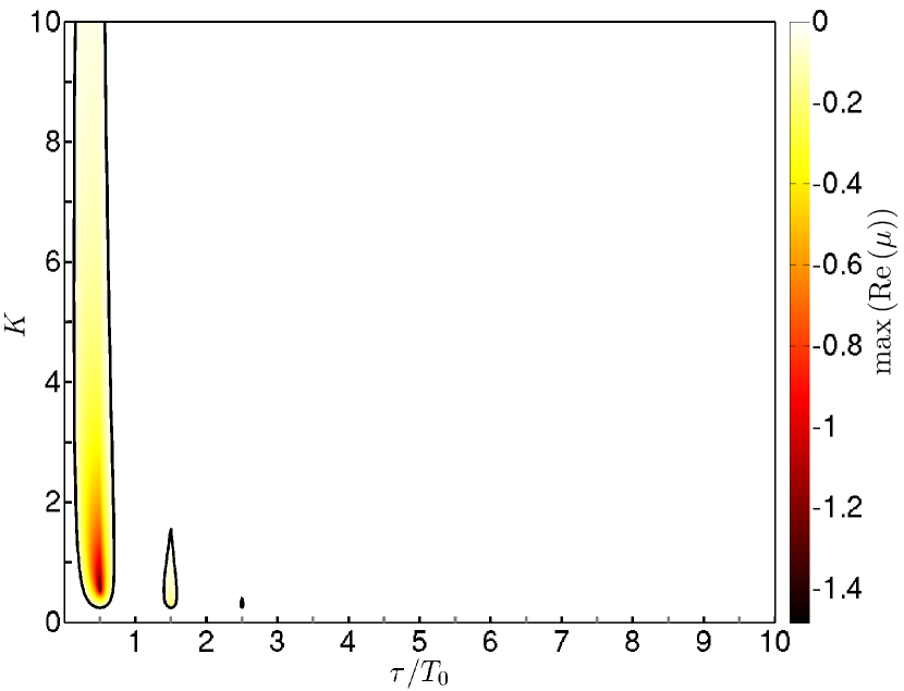
Figure 6: (Color online) Largest real part of the complex eigenvalues $\mu$ in the $K$-$\tau$ plane (only negative values are shown). The black contours bound regions where the largest real part is negative. The shear parameters are fixed to the set ${\bm{\beta}}_{\mathrm{I}}$ located within the in-plane W regime (see Fig. 1).

The black contours indicate the control parameters where the real part of the largest eigenvalue becomes zero. Within the black contours the real part is negative (colored in the plot); therefore these lines bound the regions where TDFC is successful. It is seen that the areas of stabilization shrink with increasing delay time and eventually disappear. This is due to the scaling behavior of the eigenvalue spectrum for large $\tau$ Yanchuk et al. (2006); Wolfrum et al. (2010).

IV.2 Stabilization in the isotropic phase

As a second example for the stabilization of a fixed point we now consider the reduced temperature $\theta=1.20$, at which the equilibrium (i.e., zero-shear) system is orientationally disordered. The presence of shear then induces either flow alignment or oscillatory dynamics (of type W). As seen from Fig. 2, stable W motion occurs at rather small values of the coupling parameter $\lambda_{\mathrm{K}}$ and intermediate values of the shear rate. Within this ”island” of W motion, we now focus on the parameter set ${\bm{\beta}}_{\mathrm{II}}$. The corresponding nullclines (pertaining to the components $a_{0}$, $a_{1}$, and $a_{2}$) are shown in Fig. 7.

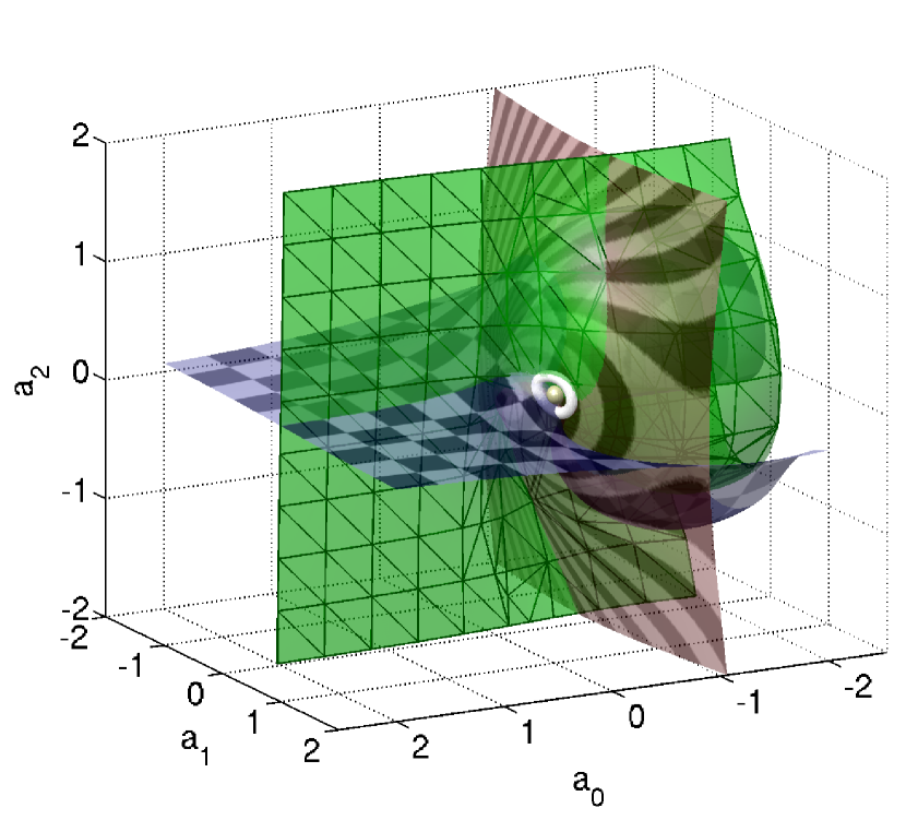
Figure 7: (Color online) Same as Fig. 3, but for the parameter set ${\bm{\beta}}_{\mathrm{II}}$ located within the island of W dynamics, which appears on shearing from the isotropic phase (see Fig. 2). The small sphere indicates the unstable fixed point, $\bm{q^{*}}_{1}=[-0.283501,0.49587,0.108511,0,0]$. The white cycle corresponds to the stable limit cycle emerging around $\bm{q}^{\star}_{1}$.

Contrary to the situation within the nematic phase discussed in the previous paragraph, we find at ${\bm{\beta}}_{\mathrm{II}}$ only one (unstable) fixed point, $\bm{q^{*}}_{1}$, and one stable limit cycle. The relevant eigenvalue of the uncontrolled system at the fixed point is given by $\nu\approx 0.027+i0.65$. From that, we find the oscillation period $T_{0}=2\pi/|\mathrm{Im}(\nu)|\approx 9.68$.

In Fig. 8a) we replot this limit cycle, supplemented by phase portraits illustrating the impact of TDFC.

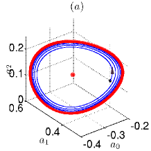
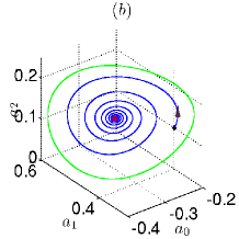
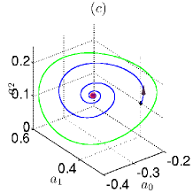
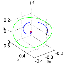
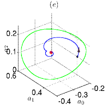
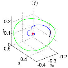
Figure 8: (Color online) Phase portraits of the dynamical variables $a_{i}$ ($i=0,1,2$). The central small dot marks the (unstable) fixed point. (a) Uncontrolled system ($K=0$) with initial condition $a_{0}^{\mathrm{init}}=-0.20$, $a_{1}^{\mathrm{init}}=0.4$, $a_{2}^{\mathrm{init}}=0.1$. (b)-(f) Systems under time-delayed feedback control [see Eq. (7)] with the control strength (b) $K=0.03$, (c) $0.05$, (d) $0.1$, (e) $0.15$, and (f) $0.2$, respectively, and delay time $\tau=5.0$. In all cases (b)-(f), the control starts at $t=0$, assuming that $a_{i}(t)=a_{i}^{\mathrm{init}}$ in the interval $[-\tau,0]$. In (a) the blue (dark) trajectory approaches a stable limit cycle, that is plotted as red (thick dark) cycle. In (b)-(f) the limit cycle of the uncontrolled system (a) is replotted for reference as green (light) cycle. For (b)-(f) all trajectories end in the fixed point. The shear parameters are fixed to the set ${\bm{\beta}}_{\mathrm{II}}$, see Fig. 2.

It is seen that the feedback control has a significant effect already at very small values of the control strength, that is, at $K=0.03$, although the chosen time delay is rather large ($\tau=5.0$). This already indicates that the system reacts more sensitively to TDFC compared to the system considered before.

The fact that small $K$ are sufficient to stabilize the fixed point is supported by the behavior of the largest real part of the eigenvalue $\mu$ plotted as function of $\tau$ in Fig. 9.

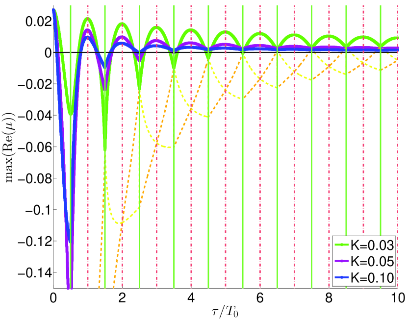
Figure 9: (Color online) Largest real part of the complex eigenvalues $\mu$ vs $\tau$ for different values of $K$ (the shear parameters are fixed to the set ${\bm{\beta}}_{\mathrm{II}}$, see Fig. 2). The dash-dotted vertical lines correspond to multiples of $T_{0}=2\pi/|\mathrm{Im}(\nu)|$ ($T_{0}\approx 9.68$), where $\nu$ is the eigenvalue of the uncontrolled system at the fixed point $\bm{q}^{\star}_{1}$ (see Fig. 7). The solid vertical lines are shifted relative to the dash-dotted lines by $T_{0}/2$. The dashed lines in the lower part indicate some lower branches of eigenvalues for $K=0.03$.

Clearly, the functions have the same qualitative behavior as those obtained in the nematic phase (see Fig. 5); however, the numerical values of $K$ are much smaller.

Finally, we present in Fig. 10 the ranges of control parameters where TDFC is successful; the boundaries have again been obtained from Eqs. (16) and (18), respectively. Compared to the nematic system, we observe a much larger number of areas where the fixed point can be stabilized. This underlines our finding that less effort is required to stabilize liquid-crystalline systems sheared from the isotropic phase, than systems sheared from the nematic phase.

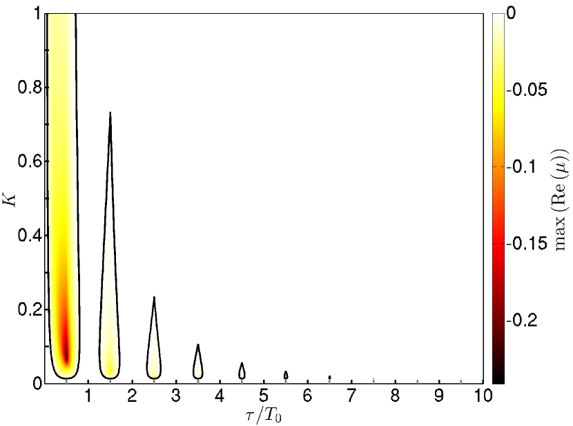
Figure 10: (Color online) Largest real part of the complex eigenvalues $\mu$ in the $K$-$\tau$ plane. The black contours bound regions where the largest real part is negative, these regions are colored, according to the colormap. The shear parameters are fixed to the set ${\bm{\beta}}_{\mathrm{II}}$, see Fig. 2.

V Conclusions

In the present paper we have discussed a five-dimensional dynamical system describing the director dynamics of sheared liquid crystal under time-delayed feedback control. The goal was to stabilize the stationary, ”flow-aligned” state for shear rates and shear coupling parameters, where the uncontrolled system performs oscillatory wagging motion in the shear plane. To this end we have applied a diagonal feedback control scheme involving a single delay time $\tau$. Following earlier theoretical work Hövel and Schöll (2005), we have analytically studied the (linear) stability problem of the controlled system, yielding explicit expressions for the domain of control. One main result is that the optimal values of control strength and delay time are closely related to the relevant complex eigenvalue of the corresponding uncontrolled system, that is, the sheared liquid crystal in the ”wagging” state. Interestingly, there is also a strong influence of the equilibrium state from which the system was sheared: in a system sheared from the isotropic phase, the control strength required to stabilize flow alignment is much smaller than in a sheared nematic system. This shows that interaction effects between the particles (which are responsible for the isotropic-nematic transition) are crucially important.

From a more general perspective, the present study thus shows that TDFC of unstable steady states, which has already been applied to a variety of optical and neural systems Dahms et al. (2010); Lehnert et al. (2011); Schöll et al. (2009); Hövel et al. (2010), is also possible and useful in the context of non-equilibrium soft-matter systems such as sheared complex fluids. In that case, stabilization of the flow-aligned state seems particularly interesting because flow-alignment is characterized by a small shear viscosity (as opposed to that of oscillatory states). Nevertheless, from a fundamental point of view it would be very interesting to extend the present analysis to the (time-delayed) feedback control of oscillatory states, which are also observed experimentally (e.g. in suspensions of tobacco viruses) Lettinga and Dhont (2004); Lettinga et al. (2005). Of course, these considerations prompt the question how a closed-loop feedback scheme such as the one proposed here could be realized experimentally.

In that context we would like to note that the ”control targets” chosen in our study, that is, the components of the order parameter tensor ${\bf a}(t)$, are related to material properties accessible in experiments. In particular, the components $a_{1}$ and $a_{2}$ are related to the so-called flow angle Hess and Kröger (2004) (i.e. the angle between the nematic director and the flow direction) and to birefringence Burghardt (1998); Kilfoil and Callaghan (2000); Cao and Berne (1993). Moreover, there is a direct relation between the alignment and the stress tensor, which can be measured in rheological experiments. This offers an additional route to extract at least some (typically non-diagonal) components of ${\bf a}$. Given that it can be difficult to monitor all components of ${\bf a}$ at once, the present diagonal control scheme, where all $a_{i}$ ($i=0,\dots,4$) are treated on the same footing, may seem too artificial. We note, however, that the control scheme could be easily modified such that only some, experimentally accessible, components of ${\bf a}$ are controlled (see Ref. Flunkert and Schöll (2011) for an application in a laser with feedback). The only drawback is that an analytical treatment is then impossible.

We further note that additive terms, such as the control terms in our TDFC scheme, also arise if the system is under the influence of an external (magnetic or electrical) field. For example, a magnetic field $\bm{H}$ would lead to an additional free energy contribution of the form $\Phi=-\bm{H}\cdot\bm{a}\cdot\bm{H}$, yielding additive terms $\propto H^{2}$ in the equation of motion [see Eq. (5)]. One idea could therefore be to choose the strength of the external field, or rather, of $H^{2}$, to be linearly dependent on the order parameters to generate a linear control scheme such as the one used here. Further possibilities to detect and thus, to control, the orientational motion could arise if the particles carry electric or magnetic moments on their own, such that time-dependent director motion directly leads to electromagnetic fields. Theoretically, the dynamical properties of such systems (without feedback control) have already been investigated Grandner et al. (2007a).

Appendix A

The components of the vector ${\bm{\Phi}}$ (consists of projections of ${\Phi^{\prime}}(\bm{a})$ on to the tensor basis)

$$\phi_{0}= ({\theta}-3a_{0}+2a^{2})a_{0}+3(a^{2}_{1}+a^{2}_{2})-{\frac{3}{2}}(a^{2}_{3}+a^{2}_{4})$$

$$\phi_{1}= ({\theta}+6a_{0}+2a^{2})a_{1}-{\frac{3}{2}}{\sqrt{3}}(a^{2}_{3}-a^{2}_{4})$$

$$\phi_{2}= ({\theta}+6a_{0}+2a^{2})a_{2}-3{\sqrt{3}}a_{3}a_{4}$$

$$\phi_{3}= ({\theta}-3a_{0}+2a^{2})a_{3}-3{\sqrt{3}}(a_{1}a_{3}+a_{2}a_{4})$$

$$\phi_{4}= ({\theta}-3a_{0}+2a^{2})a_{4}-3{\sqrt{3}}(a_{2}a_{3}-a_{1}a_{4}).$$ (19)

See also Refs. Hess and Kröger (2004); Klapp and Hess (2010); Strehober et al. (2013).

The elements of the Jacobian, $J_{ij}=\partial F_{i}/\partial q_{j}$, are given by

$$J_{00} =-(\theta-6a_{0}+4a_{0}^{2}+2a^{2})$$ (20)

$$J_{01} =-(4a_{0}a_{1}+6a_{1})$$ (21)

$$J_{02} =-(4a_{0}a_{2}+6a_{2})$$ (22)

$$J_{03} =-(4a_{0}a_{3}-3a_{3})$$ (23)

$$J_{04} =-(4a_{0}a_{4}-3a_{4}),$$ (24)

$$J_{10} =-((6+4a_{0})a_{1})$$ (25)

$$J_{11} =-(\theta+6a_{0}+2a^{2}+4a_{1}^{2})$$ (26)

$$J_{12} =-(4a_{1}a_{2})+\dot{{\gamma}}$$ (27)

$$J_{13} =-(4a_{1}a_{3}-3\sqrt{3}a_{3})$$ (28)

$$J_{14} =-(4a_{1}a_{4}+3\sqrt{3}a_{4}),$$ (29)

$$J_{20} =-((6+4a_{0})a_{2})$$ (30)

$$J_{21} =-(4a_{1}a_{2})-\dot{\gamma}$$ (31)

$$J_{22} =-(\theta+6a_{0}+2a^{2}+4a_{2}^{2})$$ (32)

$$J_{23} =-(4a_{2}a_{3}-3\sqrt{3}a_{4})$$ (33)

$$J_{24} =-(4a_{2}a_{4}-3\sqrt{3}a_{3}),$$ (34)

$$J_{30} =-((-3+4a_{0})a_{3})$$ (35)

$$J_{31} =-(4a_{1}a_{3}-3\sqrt{3}a_{3})$$ (36)

$$J_{32} =-(4a_{2}a_{3}-3\sqrt{3}a_{4})$$ (37)

$$J_{33} =-(4a_{3}^{2}-3\sqrt{3}a_{1}+(\theta-3a_{0}+2a^{2}))$$ (38)

$$J_{34} =-(4a_{4}a_{3}-3\sqrt{3}a_{2})+{\frac{1}{2}}\dot{{\gamma}},$$ (39)

$$J_{40} =-((-3+4a_{0})a_{4})$$ (40)

$$J_{41} =-(4a_{1}a_{4}+3\sqrt{3}a_{4})$$ (41)

$$J_{42} =-(4a_{2}a_{4}-3\sqrt{3}a_{3})$$ (42)

$$J_{43} =-(4a_{3}a_{4}-3\sqrt{3}a_{2})-{\frac{1}{2}}\dot{{\gamma}}$$ (43)

$$J_{44} =-(4a_{4}^{2}+3\sqrt{3}a_{1}+(\theta-3a_{0}+2a^{2})).$$ (44)

References

- Rienäcker et al. (2002a) G. Rienäcker, M. Kröger, and S. Hess, Phys. Rev. E 66, 040702(R) (2002a).
- Rienäcker et al. (2002b) G. Rienäcker, M. Kröger, and S. Hess, Physica A 315, 537 (2002b).
- Grosso et al. (2003) M. Grosso, S. Crescitelli, E. Somma, J. Vermant, P. Moldenaers, and P. L. Maffettone, Phys. Rev. Lett. 90, 098304 (2003).
- Forest et al. (2004) M. G. Forest, Q. Wang, and R. Zhou, Rheol. Acta 86, 80 (2004).
- Ripoll et al. (2008) M. Ripoll, P. Holmqvist, R. G. Winkler, G. Gompper, J. K. G. Dhont, and M. P. Lettinga, Phys. Rev. Lett. 101, 168302 (2008).
- Das et al. (2005) M. B. Das, C. Chakrabarti, S. Dasgupta, Ramaswamy, and A. K. Sood, Phys. Rev E 71, 021707 (2005).
- Hess (1975) S. Hess, Z. Naturforsch. 30a, 728 (1975).
- Hess (1976) S. Hess, Z. Naturforsch. 31a, 1034 (1976).
- Doi (1980) M. Doi, Ferroelectrics 30, 247 (1980).
- Doi (1981) M. Doi, J. Polym. Sci. Polym. Phys. Ed. 19, 229 (1981).
- Olmsted and Goldbart (1992) P. Olmsted and P. Goldbart, Phys. Rev. A 46, 4966 (1992).
- Tao et al. (2005) Y.-G. Tao, W. K. den Otter, and W. J. Briels, Phys. Rev. Lett. 95, 237802 (2005).
- Tao et al. (2009) Y. Tao, W. den Otter, and W. Briels, Europhys. Lett. 86, 56005 (2009).
- Germano and Schmid (2005) G. Germano and F. Schmid, J. Chem. Phys. 123, 214703 (2005).
- Bandyopadhyay et al. (2000) R. Bandyopadhyay, G. Basappa, and A. K. Sood, Phys. Rev. Lett. 84, 2022 (2000).
- Lettinga et al. (2005) M. P. Lettinga, Z. Dogic, H. Wang, and J. Vermant, Langmuir 21, 8048 (2005).
- Fielding (2007) S. M. Fielding, Soft Matter 3, 1262 (2007).
- Aradian and Cates (2005) A. Aradian and M. E. Cates, Europhys. Lett. 70, 397 (2005).
- Cates et al. (2002) M. E. Cates, D. A. Head, and A. Ajdari, Phys. Rev. E 66, 025202(R) (2002).
- Aradian and Cates (2006) A. Aradian and M. E. Cates, Phys. Rev. E 73, 041508 (2006).
- Goddard et al. (2008) C. Goddard, O. Hess, A. G. Balanov, and S. Hess, Phys. Rev. E 77, 026311 (2008).
- Klapp and Hess (2010) S. H. L. Klapp and S. Hess, Phys. Rev. E 81, 051711 (2010).
- Heidenreich et al. (2009) S. Heidenreich, S. Hess, and S. H. L. Klapp, Phys. Rev. Lett. 102, 028301 (2009).
- Hess and Kröger (2004) S. Hess and M. Kröger, J. Phys.: Condensed Matter 16, S3835 (2004).
- Strehober et al. (2012) D. A. Strehober, E. Schöll, and S. H. L. Klapp, AIP Conference Proceedings 1493, 552 (2012).
- Rienäcker (2000) G. Rienäcker, Orientational Dynamics of Nematic Liquid Crystals in a Shear Flow, Ph.D. thesis, TU Berlin (2000).
- Strehober et al. (2013) D. A. Strehober, H. Engel, and S. H. L. Klapp, Phys. Rev. E 88, 012505 (2013).
- de Andrade Lima and Rey (2004) L. R. P. de Andrade Lima and A. D. Rey, Phys. Rev. E 70, 011701 (2004).
- Tsuji and Rey (1997) T. Tsuji and A. D. Rey, Journal of Non-Newtonian Fluid Mechanics 73, 127 (1997).
- Rey and Denn (2002) A. D. Rey and M. M. Denn, Annual Review of Fluid Mechanics 34, 233 (2002).
- Pyragas (1992) K. Pyragas, Phys. Lett. A 170, 421 (1992).
- Baba et al. (2002) N. Baba, A. Amann, E. Schöll, and W. Just, Phys. Rev. Lett. 89, 074101 (2002).
- Unkelbach et al. (2003) J. Unkelbach, A. Amann, W. Just, and E. Schöll, Phys. Rev. E 68, 026204 (2003).
- Schlesner et al. (2003) J. Schlesner, A. Amann, N. B. Janson, W. Just, and E. Schöll, Phys. Rev. E 68, 066208 (2003).
- Kehrt et al. (2009) M. Kehrt, P. Hövel, V. Flunkert, M. A. Dahlem, P. Rodin, and E. Schöll, Eur. Phys. J. B 68, 557 (2009).
- Dahms et al. (2008) T. Dahms, P. Hövel, and E. Schöll, Phys. Rev. E 78, 056213 (2008).
- Dahms et al. (2010) T. Dahms, V. Flunkert, F. Henneberger, P. Hövel, S. Schikora, E. Schöll, and H. J. Wünsche, Eur. Phys. J. ST 191, 71 (2010).
- Schlesner et al. (2006) J. Schlesner, V. Zykov, H. Engel, and E. Schöll, Phys. Rev. E 74, 046215 (2006).
- Schlesner et al. (2008) J. Schlesner, V. S. Zykov, H. Brandstädter, I. Gerdes, and H. Engel, New J. Phys. 10, 015003 (2008).
- Kyrychko et al. (2009) Y. N. Kyrychko, K. B. Blyuss, S. J. Hogan, and E. Schöll, Chaos 19, 043126 (2009).
- Dahlem et al. (2008) M. A. Dahlem, F. M. Schneider, and E. Schöll, Chaos 18, 026110 (2008).
- Schöll et al. (2009) E. Schöll, G. Hiller, P. Hövel, and M. A. Dahlem, Phil. Trans. R. Soc. A 367, 1079 (2009).
- Panchuk et al. (2012) A. Panchuk, D. P. Rosin, P. Hövel, and E. Schöll, Int. J. Bif. Chaos (2012).
- Schöll and Schuster (2008) E. Schöll and H. G. Schuster, eds., Handbook of Chaos Control (Wiley VCH, Weinheim, 2008).
- Schöll (2009) E. Schöll, Nonlinear Dynamics of Nanosystems, edited by G. Radons, B. Rumpf, and H. G. Schuster (Wiley-VCH, Weinheim, 2009).
- Hövel and Schöll (2005) P. Hövel and E. Schöll, Phys. Rev. E 72, 046203 (2005).
- Sonnet et al. (1995) A. Sonnet, A. Kilian, and S. Hess, Phys. Rev. E 52, 718 (1995).
- Grandner et al. (2007a) S. Grandner, S. Heidenreich, S. Hess, and S. H. L. Klapp, Eur. Phys. J. E 24, 353 (2007a).
- Hess and Kröger (2005) S. Hess and M. Kröger, in Computer Simulations of Liquid Crystals and Polymers, NATO Science Series II: Mathematics, Physics and Chemistry, Vol. 177, edited by P. Pasini, C. Zannoni, and S. Zumer (Springer Netherlands, 2005) pp. 295–333.
- Grandner et al. (2007b) S. Grandner, S. Heidenreich, S. Hess, and S. H. L. Klapp, Eur. Phys. J. E 24, 353 (2007b).
- Grandner et al. (2007c) S. Grandner, S. Heidenreich, P. Ilg, S. Klapp, and S. Hess, Phys. Rev. E 75, 2 (2007c).
- de Gennes and Prost (1993) P. G. de Gennes and J. Prost, The physics of liquid crystals (Clarendon, Oxford, 1993).
- Heidenreich (2008) S. Heidenreich, Orientational Dynamics and Flow Properties of Polar and Non-Polar Hard-Rod Fluids, Ph.D. thesis, TU Berlin (2008).
- Larson and Öttinger (1991) R. G. Larson and H. C. Öttinger, Macromolecules 24, 6270 (1991).
- Corless et al. (1996) R. M. Corless, G. H. Gonnet, D. E. G. Hare, D. J. Jeffrey, and D. E. Knuth, Adv. Comput. Math. 5, 329 (1996).
- Yanchuk et al. (2006) S. Yanchuk, M. Wolfrum, P. Hövel, and E. Schöll, Phys. Rev. E 74, 026201 (2006).
- Wolfrum et al. (2010) M. Wolfrum, S. Yanchuk, P. Hövel, and E. Schöll, Eur. Phys. J. Special Topics 191, 91 (2010).
- Lehnert et al. (2011) J. Lehnert, P. Hövel, V. Flunkert, P. Y. Guzenko, A. L. Fradkov, and E. Schöll, Chaos 21, 043111 (2011).
- Hövel et al. (2010) P. Hövel, M. A. Dahlem, and E. Schöll, Int. J. Bifur. Chaos 20, 813 (2010).
- Lettinga and Dhont (2004) M. P. Lettinga and J. K. G. Dhont, J. Phys.: Condens. Matter 16, S3929 (2004).
- Burghardt (1998) W. R. Burghardt, Macromolecular Chemistry and Physics 199, 471 (1998).
- Kilfoil and Callaghan (2000) M. L. Kilfoil and P. T. Callaghan, Macromolecules 33, 6828 (2000).
- Cao and Berne (1993) J. Cao and B. J. Berne, J. Chem. Phys. 99, 2213 (1993).
- Flunkert and Schöll (2011) V. Flunkert and E. Schöll, Phys. Rev. E 84, 016214 (2011).