Non-collective excitations in low-energy heavy-ion reactions: applicability of the random-matrix model

Abstract

We investigate the applicability of a random-matrix model to the description of non-collective excitations in heavy-ion reactions around the Coulomb barrier. To this end, we study fusion in the reaction ¹⁶O + ²⁰⁸Pb, taking account of the known non-collective excitations in the ²⁰⁸Pb nucleus. We show that the random-matrix model for the corresponding couplings reproduces reasonably well the exact calculations, obtained using empirical deformation parameters. This implies that the model may provide a powerful method for systems in which the non-collective couplings are not so well known.

I Introduction

Heavy-ion reactions around the Coulomb barrier often show a behavior that cannot be accounted for by a simple potential model dasgupta ; BT98 ; HT12 . They have thus provided a good opportunity to investigate the role of internal degrees of freedom in the reaction process. One of the well known examples is a large enhancement of sub-barrier fusion cross sections due to the couplings between the relative motion of the projectile and target nuclei and their internal degrees of freedom, such as surface vibrations for spherical nuclei, or rotational motion for nuclei possessing a static, intrinsic deformation. It is well recognized that these couplings lead to a distribution of potential barriers DLW83 , and a method was proposed by Rowley, Satchler and Stelson to extract the barrier distributions directly from experimental fusion cross sections RSS91 . The barrier distributions extracted in this way are found to be sensitive to details of the couplings, often showing a characteristic structured behavior dasgupta ; L95 ; LRL93 . Similar heavy-ion barrier distributions can also be defined for large-angle quasi-elastic scattering timmers ; HR04 .

In order to analyze experimental data for these low-energy heavy-ion reactions, the coupled-channels method has been employed as a standard approach ccfull ; HT12 . This method describes the reaction in terms of the internal excitations of the colliding nuclei, representing the total wave function of the system as a superposition of wave functions for the relevant reaction channels. Conventionally, a few low-lying collective excitations, that are strongly coupled to the ground state, are taken into account in these calculations. Such analyses have successfully accounted for the strong enhancement of sub-barrier fusion cross sections, and have successfully reproduced the structure of the fusion and quasi-elastic barrier distributions for many systems dasgupta ; HT12 .

Recently, quasi-elastic barrier distributions have been measured for the ²⁰Ne +^90,92Zr systems piasecki . The corresponding coupled-channels calculations show that the main structure of these barrier distributions is determined by the rotational excitations of the strongly deformed nucleus ²⁰Ne. The calculated barrier distributions are in fact almost identical for the two systems, even when the collective excitations of the Zr isotopes are taken into account. It was, therefore, surprising when the two experimental barrier distributions were found to be different in an important respect. That is, the barrier distribution for ²⁰Ne + ⁹²Zr exhibits a much more smeared behavior than that for the ²⁰Ne + ⁹²Zr system. The origin of this difference has been conjectured in Ref. piasecki to be the multitude of non-collective excitations of the Zr isotopes, that are generally ignored in a coupled-channels analysis. In fact, the two extra neutrons in the ⁹²Zr nucleus lead to a significantly larger number of non-collective excited states compared with ⁹⁰Zr, since this latter possesses an $N=50$ closed shell (the difference is reflected by the number of known states up to an excitation energy of 5 MeV; one finds 35 for ⁹⁰Zr and 87 for ⁹²Zr bnl ).

There are many ways to describe non-collective excitations in heavy-ion reactions YHR10 ; YHR12 ; DHD08 ; B10 ; B102 ; KPW76 ; AKW78 ; BSW78 ; akw1 ; akw2 ; akw3 ; akw4 . In the 1970’s, Weidenmüller et al. introduced a random-matrix model for such excitations in order to study deep inelastic collisions KPW76 ; AKW78 ; BSW78 ; akw1 ; akw2 ; akw3 ; akw4 . In Ref. YHR10 , we have used a similar model in a schematic one-dimensional barrier-penetration problem, in order to study the role of these non-collective excitations in low-energy reactions. On the other hand, in Ref. YHR12 , we have explicitly taken into account in the coupled-channels formalism all of the 70 known non-collective states in ²⁰⁸Pb below 7.382 MeV WCHM75 ; LBF73 without resorting to the random-matrix model, and have analysed in this way the experimental data for the ¹⁶O+²⁰⁸Pb reaction. Although some discrepancies between the experimental and theoretical barrier distributions remain after the inclusion of non-collective excitations, we have shown in Ref. YHR12 that these excitations play a more important role as the incident energy increases. We have also compared there the role of non-collective excitations in the fusion and quasi-elastic barrier distributions, and have shown that they affect both distributions in a similar fashion.

Given that exact calculations with a realistic spectrum for non-collective states is possible here, it is intriguing to also apply the random-matrix model to this system in order to test its applicability. This theoretical test is the main aim of this paper, and we achieve it by comparing our new results with those obtained in Ref. YHR12 . Note that, in contrast to ²⁰⁸Pb, the properties of the non-collective states in ^90,92Zr are not known sufficiently well. As we will show in this paper, the random-matrix model provides a good method for a description of non-collective excitations in such a situation.

The paper is organized as follows. In Sec. II, we explain the coupled-channels formalism with non-collective excitations based on the random-matrix model. In Sec. III, we discuss the strength distribution and fusion cross sections obtained with this model. We then compare these with calculations using the more exact couplings and discuss the applicability of the random-matrix model. The paper is summarised in Sec. IV.

II Coupled-channels method with non-collective excitations

In order to describe internal excitations during the reaction process, we assume the following Hamiltonian,

$$H=-\frac{\hbar^{2}}{2\mu}\nabla^{2}+V_{\rm rel}(r)+H_{0}(\{\xi\})+V_{\rm coup}(\mbox{\boldmath$r$},\{\xi\}),$$ (1)

where $r$ is the separation of the projectile and target nuclei, and $\mu$ is the reduced mass. In this equation, $H_{0}(\{\xi\})$ is the intrinsic Hamiltonian with $\{\xi\}$ representing a set of internal degrees of freedom. The optical potential for the relative motion is $V_{\rm rel}(r)$, and it includes an imaginary part to simulate the fusion process (that is, strong absorption into compound-nucleus degrees of freedom inside the Coulomb barrier). The coupling Hamiltonian between the relative motion and the intrinsic degrees of freedom is denoted by $V_{\rm coup}(\mbox{\boldmath$r$},\{\xi\})$.

The coupled-channels equations for this Hamiltonian are obtained by expanding the total wave function in terms of the eigenfunctions of $H_{0}(\{\xi\})$. The equations read,

$$\left[-\frac{\hbar^{2}}{2\mu}\frac{d^{2}}{dr^{2}}+\frac{J(J+1)\hbar^{2}}{2\mu r^{2}}+V_{\rm rel}(r)+\epsilon_{n}-E\right]u_{n}^{J}(r)$$

$$+\sum_{m}V_{nm}(r)u_{m}^{J}(r)=0,$$ (2)

where $\epsilon_{n}$ is the excitation energy for the $n$-th channel. In deriving these equations, we have employed the iso-centrifugal approximation HT12 ; LR84 ; NRL86 ; NBT86 ; ELP87 ; T87 ; GAN94 . In this approximation, the orbital angular momentum in the centrifugal potential is replaced by the total angular momentum $J$, thereby considerably reducing the dimension of the coupled-channels equations.

In solving these equations, we impose the following asymptotic boundary conditions,

$$u_{n}^{J}(r)\rightarrow H_{J}^{(-)}(k_{n}r)\delta_{n,0}-\sqrt{\frac{k_{0}}{k_{n}}}S_{n}^{J}H_{J}^{(+)}(k_{n}r),$$ (3)

for $r\rightarrow\infty$, together with the regular boundary condition at the origin. Here, $k_{n}=\sqrt{2\mu(E-\epsilon_{n})/\hbar^{2}}$ is the wave number for the $n$-th channel, where $n=0$ corresponds to the entrance channel. $S_{n}^{J}$ is the nuclear $S$-matrix, and $H_{J}^{(-)}(kr)$ and $H_{J}^{(+)}(kr)$ are the incoming and the outgoing Coulomb wave functions, respectively. The fusion cross sections are then obtained as

$$\sigma_{\rm fus}(E)=\frac{\pi}{k_{0}^{2}}\sum_{J}(2J+1)\left(1-\sum_{n}\left|S_{n}^{J}\right|^{2}\right).$$ (4)

In the random-matrix model KPW76 ; AKW78 ; BSW78 ; akw1 ; akw2 ; akw3 ; akw4 , one assumes an ensemble of coupling matrix elements whose first moment satisfies

$$\overline{V_{nn^{\prime}}^{II^{\prime}}(r)}=0,$$ (5)

while the second moment satisfies

$$\ \ \ \ \ \overline{V_{nn^{\prime}}^{II^{\prime}}(r)V_{n^{\prime\prime}n^{\prime\prime\prime}}^{I^{\prime\prime}I^{\prime\prime\prime}}(r^{\prime})}$$

$$=\left\{\delta_{nn^{\prime\prime}}\delta_{n^{\prime}n^{\prime\prime\prime}}\delta_{II^{\prime\prime}}\delta_{I^{\prime}I^{\prime\prime\prime}}+\delta_{nn^{\prime\prime\prime}}\delta_{n^{\prime}{n^{\prime\prime}}}\delta_{II^{\prime\prime\prime}}\delta_{I^{\prime}{I^{\prime\prime}}}\right\}$$

$$\ \ \ \ \times\sqrt{(2I+1)(2I^{\prime}+1)}\,\sum_{\lambda}\left(\begin{array}[]{ccc}I&\lambda&I^{\prime}\\ 0&0&0\end{array}\right)^{2}$$ (8)

$$\ \ \ \ \times\alpha_{\lambda}(n,n^{\prime};I,I^{\prime};r,r^{\prime}).$$ (9)

Here, $I$ is the spin of the intrinsic state labeled by $n$, and $\alpha_{\lambda}$ is the coupling form factor.

In this paper, for simplicitly, we assume that the non-collective excitations couple only to the ground state, as in the linear coupling approximation employed in our previous work YHR12 . For the form factor $\alpha_{\lambda}$, we assume the following dependence

$$\alpha_{\lambda}(n,0;I,0;r,r^{\prime})=\frac{w_{\lambda}}{\sqrt{\rho(\epsilon_{n})}}e^{-\frac{\epsilon_{n}^{2}}{2\Delta^{2}}}e^{-\frac{(r-r^{\prime})^{2}}{2\sigma^{2}}}h(r)h(r^{\prime}),$$ (10)

where $\rho(\epsilon_{n})$ is the level density at an excitation energy $\epsilon_{n}$, and ($w_{\lambda},\Delta,\sigma$) are adjustable parameters. The appearance of the level density in the denominator reflects the complexity of the non-collective excited states, as discussed in Ref. akw1 . For the function $h(r)$, we adopt the derivative of the Woods-Saxon potential, that is,

$$h(r)=\frac{e^{(r-R)/a}}{\left[1+e^{(r-R)/a}\right]^{2}}.$$ (11)

Note that this choice of the form factor corresponds to the coupling Hamiltonian in the linear coupling approximation derived from the Woods-Saxon potential.

III Applicability of random-matrix model

III.1 Strength distribution

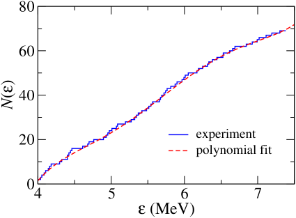
Figure 1: (Color online) The number of levels of the ²⁰⁸Pb nucleus up to the excitation energy $\epsilon$ as a function of $\epsilon$. The histogram represents the experimental data WCHM75 , while the dashed line shows its fit with a polynomial function up to the sixth order.

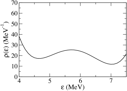
Figure 2: The continuous level density for ²⁰⁸Pb obtained as a first derivative of the fitting function $f(\epsilon)$ shown in Fig. 2.

Let us now apply the random-matrix model to the ¹⁶O+²⁰⁸Pb reaction and discuss its applicability. We first discuss the strength distribution for the non-collective excitations in ²⁰⁸Pb obtained with the random-matrix model. To this end, we define the strength distribution as

$$b_{I} =\sqrt{\sum_{\lambda}\left(\begin{array}[]{ccc}0&\lambda&I\\ 0&0&0\end{array}\right)^{2}\sqrt{\frac{2I+1}{\rho(\epsilon)}}e^{-\frac{\epsilon^{2}}{2\Delta^{2}}}}$$ (14)

$$=\sqrt{\sqrt{\frac{2I+1}{\rho(\epsilon)}}e^{-\frac{\epsilon^{2}}{2\Delta^{2}}}}.$$ (15)

This quantity essentially corresponds to the “square root”  of Eq. (9), except for an overall scale factor (here we have assumed $w_{\lambda}=w$ for all $\lambda$ and omitted $w_{\lambda}$ in the definition for the strength function).

The level density in Eq. (15) is treated in the following way. It is originally defined by

$$\rho(\epsilon)=\sum_{n}\delta(\epsilon-\epsilon_{n})$$ (16)

for a discrete spectrum. For practical purposes, we define the function

$$N(\epsilon)=\int^{\epsilon}_{0}\rho(\epsilon^{\prime})d\epsilon^{\prime}=\sum_{n}\theta(\epsilon-\epsilon_{n}),$$ (17)

that gives the number of levels up to the excitation energy $\epsilon$. We fit this function with a polynomial in $\epsilon$, and then define a continuous level density by differentiating this polynomial. Figure 2 shows the experimental $N(\epsilon)$ for ²⁰⁸Pb WCHM75 in the interval between 4 MeV and 7.5 MeV (solid line) and its fit with a polynomial $\displaystyle f(\epsilon)=\sum_{n=0}^{6}a_{n}\epsilon^{n}$ (dashed line). The values of $a_{n}$ are $a_{0}=-7479,a_{1}=6969$ (MeV^-1), $a_{2}=-2612$ (MeV^-2), $a_{3}=497.5$ (MeV^-3), $a_{4}=-49.59$ (MeV^-4), $a_{5}=2.347$ (MeV^-5), and $a_{6}=-0.03632$ (MeV^-6). The continuous level density, $\rho(\epsilon)=df(\epsilon)/d\epsilon$, is shown in Fig. 2.

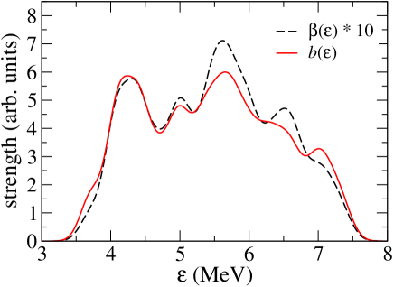
Figure 3: (Color online) The strength distributions for ²⁰⁸Pb as a function of excitation energy $\epsilon$. The dashed line shows the distribution of the experimental deformation parameters, while the solid line is obtained based on the random-matrix model using Eq. (15). Both distributions are smeared with a Gaussian function with a width of 0.15 MeV. An overall scaling factor is introduced to the dashed line as the dimension is different between the two curves (see text).

The strength distribution $b_{I}$ calculated with this level density is shown in Fig. 3 by the solid line as a function of excitation energy $\epsilon$. The parameter $\Delta$ in Eq. (15) is chosen to be 7 MeV, as in Refs. akw3 ; akw4 . For comparison, the figure also shows the distribution of the experimental deformation parameters $\beta_{I}$ WCHM75 , smeared with a gaussian function with a width of 0.15 MeV (dashed line). We have also performed the same smearing for the strength distribution $b_{I}$. Also, since the dimensions of $\beta_{I}$ and $b_{I}$ are not the same, the deformation parameters $\beta_{I}$ are scaled by a factor 10 so that the heights of the first peaks at about 4.3 MeV match one another. Although there exists a small deviation for the peaks between 5 MeV and 7 MeV, the overall structure of the strength distribution is well reproduced by this model.

III.2 Fusion cross sections

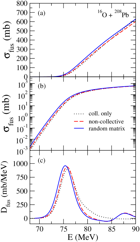
Figure 4: (Color online) (a) and (b) Fusion cross sections $\sigma_{\rm fus}$ and (c) fusion barrier distributions $D_{\rm fus}(E)=d^{2}{E\sigma_{\rm fus}(E)}{dE^{2}}$ for the ¹⁶O + ²⁰⁸Pb system obtained from three different calculations. Dashed lines show results obtained with the experimental, non-collective deformation parameters, whereas the solid lines are obtained from the random-matrix model. Dotted lines result from calculations that include only the ²⁰⁸Pb collective excitations.

The strength distribution discussed in the previous subsection determines the coupling strength to each excited state. Let us then examine how the random-matrix model can be compared with the exact results in terms of the fusion cross sections for the ¹⁶O + ²⁰⁸Pb system. For this purpose, we use the same Woods-Saxon potential for the nuclear potential as in Ref. YHR12 ; it has a surface diffuseness $a=0.671$ fm, a radius $R=8.39$ fm and a depth $V_{0}$ = 550 MeV. For the couplings to the collective excitations, we take into account the vibrational $3^{-}$ state at 2.615 MeV, the $5^{-}$ state at 3.198 MeV, and the $2^{+}$ state at 4.085 MeV in ²⁰⁸Pb. The octupole mode is included up to the two-phonon states, while the other, weaker, vibrational modes are taken into account only up to their one-phonon states. The deformation parameters for these vibrational modes are estimated from the measured electromagnetic transition probabilities. They are $\beta_{3}$ = 0.122, $\beta_{5}$ = 0.058, and $\beta_{2}$ = 0.058 together with a radius parameter of $r_{0}$=1.2 fm. Although we took into account the octupole phonon state of ¹⁶O in our preivous study YHR12 , for simplicity we do not include it in the present calculations, since its effect can be well described by an adiabatic renormalization of the potential depth HT12 ; THAB94 . For the parameter $\sigma$ in Eq. (10), we follow Refs. akw3 ; akw4 and use $\sigma=4$ fm. On the other hand, the parameter $w_{\lambda}=w$ is chosen to be $w=38000$ MeV^3/2 so that the height of the main peak in the fusion barrier distribution is reproduced by the random-matrix model.

Figures 4 (a) and 4 (b) show the ¹⁶O+²⁰⁸Pb fusion excitation function on linear and logarithmic scales respectively. The dashed lines show the results obtained with the measured deformation parameters for the non-collective excitations, while the solid lines show the results obtained using the random-matrix approximation. For comparison, the dotted lines show results that account only for the collective excitations. Although a small overall shift can be seen, it is clear that the random-matrix model reproduces the exact results reasonably well.

In order to highlight the energy dependence, Fig. 4 (c) shows the fusion barrier distribution $D_{\rm fus}(E)=d^{2}(E\sigma_{\rm fus})/dE^{2}$ dasgupta ; HT12 ; RSS91 ; L95 . Although the main peak is slightly shifted in energy, this confirms that the random-matrix model reproduces well the exact results. That is, with respect to the dotted line, the change in the energy dependence of fusion cross sections due to the non-collective excitations is similar in the two calculations. In particular, both barrier distributions are smeared out in a similar way at energies around 80 MeV, and both calculations yield a similar second peak around 87.5 MeV. (We note that if the strength $w_{0}$ was somewhat larger, the second peak could appear at even higher energies, possibly reflecting the broad bump seen at around 97 MeV in the experimental data.)

As we have argued in Ref. YHR10 , the higher-energy peaks in the barrier distribution are affected more by non-collective excitations than are the lower-energy peaks. Unfortunately this is not easy to see in Fig. 4 because the peaks obtained with purely collective couplings are not resolved. This difference can, however, be easily understood using perturbation theory. That is, the eigenchannels corresponding to the higher-energy peaks in the barrier distribution couple more strongly to the non-collective states via their ground state component simply because the energy differences are smaller. Higher peaks are thus redistributed more, effectively removing much of their strength from that region of energy.

From these calculations, it is evident that the effects of non-collective excitations are not sensitive to details of the non-collective couplings, and that the random-matrix model is applicable to the description of non-collective excitations, so long as the relevant parameters are chosen appropriately.

IV Summary

We have investigated the applicability of the random-matrix model for the description of non-collective excitations in low-energy heavy-ion reactions. To this end, we have calculated the fusion excitation function for the ¹⁶O +²⁰⁸Pb system, where the role of the non-collective excitations has already been investigated in our previous study using empirical deformation parameters.

We have first shown that the coupling strength distribution obtained with the random-matrix model agrees well with the experimental distribution. The fusion cross section and barrier distribution for the ¹⁶O + ²⁰⁸Pb system obtained with empirical non-collective couplings are also well reproduced by the random-matrix model with appropriately chosen parameters. These results provide a validation of the random-matrix model for the description of non-collective couplings.

For the ²⁰⁸Pb nucleus, detailed properties of non-collective states are known over a large energy range. However, this is not always the case for other systems. That is, for many nuclei, even though the energies and spin-parity may be relatively well known for many non-collective states, the coupling strengths are poorly determined. In such a situation, the present study suggests that the random matrix model provides a powerful tool to treat these coupling strengths. A good example is the quasi-elastic barrier distribution for the ²⁰Ne + ^90,92Zr systems, where it has been suggested that non-collective excitations may play an important role. Analyses for these systems within the random-matrix model are under way. We shall report the results in a separate publication YHR13 .

- (1) M. Dasgupta, D.J. Hinde, N. Rowley, and A.M. Stefanini, Annu. Rev. Nucl. Part. Sci. 48, 401(1998).
- (2) A. B. Balantekin and N. Takigawa, Rev. Mod. Phys. 70, 77(1998).
- (3) K. Hagino and N. Takigawa, Prog. Theor. Phys., 128, 1061 (2012).
- (4) C.H. Dasso, S. Landowne, and A. Winther, Nucl. Phys. A405, 381 (1983); A407, 221 (1983).
- (5) N. Rowley, G.R. Satchler and P.H. Stelson, Phys. Lett. B254 25, (1991).
- (6) J.R. Leigh et al., Phys. Rev. C52, 3151 (1995).
- (7) J. R. Leigh, N. Rowley, R. C. Lemmon, D. J. Hinde, J. O. Newton, J. X. Wei, J. C. Mein, C. R. Morton, S. Kuyucak, and A. T. Kruppa, Phys. Rev. C47, R437(1993).
- (8) H. Timmers, J.R. Leigh, M. Dasgupta, D.J. Hinde, R.C. Lemmon, J.C. Mein, C.R. Morton, J.O. Newton, and N. Rowley, Nucl. Phys. A584, 190 (1995).
- (9) K. Hagino and N. Rowley, Phys. Rev.C 69, 054610(2004).
- (10) K. Hagino, N. Rowley, A. T. Kruppa, Compt. Phys. Comm. 123, 143 (1999).
- (11) E. Piasecki, Ł. Świderski, W. Gawlikowicz, J. Jastrzebski, N. Keeley, M. Kisieliński, S. Kliczewski, A. Kordyasz, M. Kowalczyk, S. Khlebnikov, E. Koshchiy, E. Kozulin, T. Krogulski, T. Loktev, M. Mutterer, K. Piasecki, A. Piórkowska, K. Rusek, A. Staudt, M. Sillanpää, S. Smirnov, I. Strojek, G. Tiourin, W. H. Trzaska, A. Trzcińska, K. Hagino, and N. Rowley, Phys. Rev. C80, 054613 (2009).
- (12) Brookhaven National Laboratory, Evaluated Nuclear Structure Data File, http://www.nndc.bnl.gov/ensdf/, and references therein.
- (13) S. Yusa, K. Hagino, and N. Rowley, Phys. Rev. C82, 024606(2010).
- (14) S. Yusa, K. Hagino, and N. Rowley, Phys. Rev. C85, 054601(2012).
- (15) A. Diaz-Torres, D. J. Hinde, M. Dasgupta, G. J. Milburn, and J. A. Tostevin, Phys. Rev. C 78, 064604 (2008).
- (16) A. Diaz-Torres, Phys. Rev. C 81, 041603(R) (2010).
- (17) A. Diaz-Torres, Phys. Rev. C 82, 054617 (2010).
- (18) C. M. Ko, H. J. Pirner, and H. A. Weidenmüller, Phys. Lett. 62B, 248 (1976).
- (19) D. Agassi, H. A. Weidenmüller, and C. M. Ko, Phys. Lett. 73B, 284 (1978).
- (20) B. R. Barrett, S. Shlomo, and H. A. Weidenmüller, Phys. Rev. C 17, 544 (1978).
- (21) D. Agassi, C.M. Ko, and H.A. Weidenmüller, Ann. Phys 107, 140(1977).
- (22) C.M. Ko, D. Agassi, and H.A. Weidenmüller, Ann. Phys 117, 237(1979).
- (23) D. Agassi, C.M. Ko, and H.A. Weidenmüller, Ann. Phys 117, 407 (1979).
- (24) D. Agassi, C.M. Ko, and H.A. Weidenmüller, Phys. Rev. C 18, 223(1978).
- (25) W. T. Wagner, G. M. Crawley, G. R. Hammerstein, and H. McManus, Phys. Rev. C12, 757(1975).
- (26) M. B. Lewis, F. E. Bertrand, and C. B. Fulmer, Phys. Rev. C7, 1966(1973).
- (27) R. Lindsay and N. Rowley, J. Phys. G10, 805 (1984).
- (28) M.A. Nagarajan, N. Rowley, and R. Lindsay, J. Phys. G12, 529 (1986).
- (29) M.A. Nagarajan, A.B. Balantekin, and N. Takigawa, Phys. Rev. C34, 894 (1986).
- (30) H. Esbensen, S. Landowne, and C. Price, Phys. Rev. C36, 1216 (1987); C36, 2359 (1987).
- (31) O. Tanimura, Phys. Rev. C35, 1600 (1987); Z. Phys. A327, 413 (1987).
- (32) J. Gomez-Camacho, M.V. Andres, and M.A. Nagarajan, Nucl. Phys. A580, 156 (1994).
- (33) N. Takigawa, K. Hagino, M. Abe, and A.B. Balantekin, Phys. Rev. C49, 2630 (1994).
- (34) S. Yusa, K. Hagino, and N. Rowley, to be published.