Partial differential equation about the prevalence of a chronic disease in the presence of duration dependency

Ralph Brinks
Abstract

The illness-death model of a chronic disease consists of the states Normal, Disease, and Death. In general, the transition rates between the states depend on three time scales: calendar time, age and duration of the chronic disease. Previous works have shown that the age-specific prevalence of the chronic disease can be described by differential equations [2, 4] if the duration is negligible. This article derives a partial differential equation (PDE) in the presence of duration dependency. As an important application, the PDE allows the calculation of the age-specific incidence from cross-sectional surveys.

1 Introduction

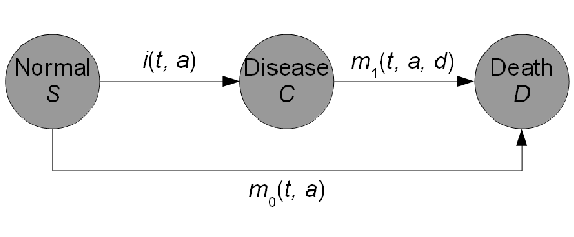
The articles [2] and [4] deal with the illness-death model as shown in Figure 1. The model describes a population consisting of healthy and ill persons with respect to a chronic (i.e., irreversible) disease. Let the number of persons in the states Normal and Disease be denoted with S𝑆S and C𝐢C. The transition rates between the states are the incidence rate i𝑖i and the mortality rates m0subscriptπ‘š0m_{0} and m1subscriptπ‘š1m_{1} of the healthy and the diseased persons, respectively. In general, these rates depend on the calendar time t𝑑t, on the age aπ‘Ža and in case of m1subscriptπ‘š1m_{1} also on the duration d𝑑d.

Refer to caption
Figure 1: Illness-death model with three states and the associated transition rates. Persons in the state Normal do not have the chronic disease. In case of an onset, they change to the state Disease.

The articles [2] and [4] derived differential equations (DEs) about the age-specific prevalence p=CC+S𝑝𝐢𝐢𝑆p=\tfrac{C}{C+S} and the rates i𝑖i, m0subscriptπ‘š0m_{0} and m1::subscriptπ‘š1absentm_{1}:

(1) βˆ‚p=(1βˆ’p)​(iβˆ’p​(m1βˆ’m0)).𝑝1𝑝𝑖𝑝subscriptπ‘š1subscriptπ‘š0\partial p=(1-p)\,\left(i-p\left(m_{1}-m_{0}\right)\right).

The symbol βˆ‚\partial means a differential operator, either βˆ‚=dd​addπ‘Ž\partial=\tfrac{\mathrm{d}}{\mathrm{d}a} or βˆ‚=βˆ‚βˆ‚t+βˆ‚βˆ‚a,π‘‘π‘Ž\partial=\tfrac{\partial}{\partial t}+\tfrac{\partial}{\partial a}, depending on the setting.


The advantages of an equation of the form (1) is the relatively simple relation between the rates i,m0,m1𝑖subscriptπ‘š0subscriptπ‘š1i,m_{0},m_{1} and the prevalence p𝑝p. If the rates on the right hand side of the equation are known, the DE can be solved for p𝑝p. This is called the direct problem [3]. Furthermore, if p,m0𝑝subscriptπ‘š0p,m_{0} and m1subscriptπ‘š1m_{1} are known, Equation (1) can be solved for the incidence i𝑖i. This inverse problem allows the calculation of the incidence of a chronic disease from cross-sectional data. Usually in epidemiology, incidence rates are surveyed by lengthy (and thus expensive) follow-up studies. The possibility to use less complex cross-sectional data instead of follow-up studies is an enormous benefit and has been requested for a long time (see [7] for an overview).


The DEs in [2, 4] were restricted to the case of m1subscriptπ‘š1m_{1} being independent from the disease duration d𝑑d. For some chronic diseases, this is not the case. An example is type 2 diabetes: after physiological onset, most patients do not have any symptoms and the disease remains undetected. After onset of clinical symptoms, the mortality already m1subscriptπ‘š1m_{1} is higher compared to the mortality m0subscriptπ‘š0m_{0} of a healthy person with the same age (and sex). Then, the therapy starts. During therapy, the mortality decreases and after some time with the disease the mortality increases again due to late sequelae. In the Danish diabetes register the J-shaped mortality ratio (i.e., m1m0subscriptπ‘š1subscriptπ‘š0\tfrac{m_{1}}{m_{0}}) is empirically evident [5]. There are other chronic diseases with duration being an important factor for mortality, for example, dementia [10] and systemic lupus erythematosus [1]. It is likely that duration is an important covariate for many of chronic diseases.

The aim of this article is the derivation of a partial differential equation (PDE) similar to Equation (1) in case the mortality rate m1subscriptπ‘š1m_{1} depends on the duration d𝑑d. Thus, this work is a generalization of the the previous articles [2, 4].

2 Basic equations for the illness-death model

As in [4] let S​(t,a)π‘†π‘‘π‘ŽS(t,a) and C​(t,a)πΆπ‘‘π‘ŽC(t,a) denote the numbers of healthy and diseased persons aged aπ‘Ža at time t𝑑t. Based on the possible transitions from the Normal state in Figure 1 we get the following Cauchy problem for S​(t,a)π‘†π‘‘π‘ŽS(t,a):

(2) (βˆ‚t+βˆ‚a)​S​(t,a)subscript𝑑subscriptπ‘Žπ‘†π‘‘π‘Ž\displaystyle(\partial_{t}+\partial_{a})\,S(t,a) =\displaystyle= βˆ’(m0​(t,a)+i​(t,a))​S​(t,a)subscriptπ‘š0π‘‘π‘Žπ‘–π‘‘π‘Žπ‘†π‘‘π‘Ž\displaystyle-\left(m_{0}(t,a)+i(t,a)\right)\,S(t,a)
S​(tβˆ’a,0)π‘†π‘‘π‘Ž0\displaystyle S(t-a,0) =\displaystyle= S0​(tβˆ’a).subscript𝑆0π‘‘π‘Ž\displaystyle S_{0}(t-a).

Here S0​(tβˆ’a)=S​(tβˆ’a,0)subscript𝑆0π‘‘π‘Žπ‘†π‘‘π‘Ž0S_{0}(t-a)=S(t-a,0) is the number of healthy newborns at calendar time tβˆ’aπ‘‘π‘Žt-a. Henceforth, the notation βˆ‚xsubscriptπ‘₯\partial_{x} means the partial derivative for the variable x,x∈{t,a,d}.π‘₯π‘₯π‘‘π‘Žπ‘‘x,~{}x\in\{t,a,d\}. The rates i,m0𝑖subscriptπ‘š0i,m_{0} and m1subscriptπ‘š1m_{1} in Figure 1 are assumed to be sufficiently smooth, such that the common uniqueness and existence theorems hold [9].

The unique solution S​(t,a)π‘†π‘‘π‘ŽS(t,a) is

(3) S​(t,a)=S0​(tβˆ’a)​exp⁑(βˆ’βˆ«0am0​(tβˆ’a+Ο„,Ο„)+i​(tβˆ’a+Ο„,Ο„)​d​τ).π‘†π‘‘π‘Žsubscript𝑆0π‘‘π‘Žsuperscriptsubscript0π‘Žsubscriptπ‘š0π‘‘π‘Žπœπœπ‘–π‘‘π‘Žπœπœd𝜏S(t,a)=S_{0}(t-a)\,\exp\left(-\int_{0}^{a}m_{0}(t-a+\tau,\tau)+i(t-a+\tau,\tau)\,\mathrm{d}\tau\right).

In case of the diseased persons, we have to distinguish between different disease durations. Let C⋆​(t,a,d)superscriptπΆβ‹†π‘‘π‘Žπ‘‘C^{\star}(t,a,d) be the number of diseased persons aged aπ‘Ža at time t𝑑t having the disease for the exact duration d,d<a.π‘‘π‘‘π‘Žd,~{}d<a.

For C⋆​(t,a,d)superscriptπΆβ‹†π‘‘π‘Žπ‘‘C^{\star}(t,a,d) we also have a PDE:

(4) (βˆ‚t+βˆ‚a+βˆ‚d)​C⋆​(t,a,d)=βˆ’C⋆​(t,a,d)​m1​(t,a,d).subscript𝑑subscriptπ‘Žsubscript𝑑superscriptπΆβ‹†π‘‘π‘Žπ‘‘superscriptπΆβ‹†π‘‘π‘Žπ‘‘subscriptπ‘š1π‘‘π‘Žπ‘‘(\partial_{t}+\partial_{a}+\partial_{d})\,C^{\star}(t,a,d)=-C^{\star}(t,a,d)\,m_{1}(t,a,d).

The initial condition for making Equation (4) a Cauchy problem stems from the assumption that newly diseased persons may only enter from the Normal state. This means: C⋆​(t,a,0)=i​(t,a)​S​(t,a)superscriptπΆβ‹†π‘‘π‘Ž0π‘–π‘‘π‘Žπ‘†π‘‘π‘ŽC^{\star}(t,a,0)=i(t,a)\,S(t,a) for all t,a.π‘‘π‘Žt,a.

The unique solution of the Cauchy problem for C⋆​(t,a,d)superscriptπΆβ‹†π‘‘π‘Žπ‘‘C^{\star}(t,a,d) is:

C⋆​(t,a,d)superscriptπΆβ‹†π‘‘π‘Žπ‘‘\displaystyle C^{\star}(t,a,d) =\displaystyle= C⋆​(tβˆ’d,aβˆ’d,0)​exp⁑(βˆ’βˆ«0dm1​(tβˆ’d+Ο„,aβˆ’d+Ο„,Ο„)​dΟ„)superscriptπΆβ‹†π‘‘π‘‘π‘Žπ‘‘0superscriptsubscript0𝑑subscriptπ‘š1π‘‘π‘‘πœπ‘Žπ‘‘πœπœdifferential-d𝜏\displaystyle C^{\star}(t-d,a-d,0)\,\exp\left(-\int_{0}^{d}m_{1}(t-d+\tau,a-d+\tau,\tau)\,\mathrm{d}\tau\right)
=\displaystyle= i​(tβˆ’d,aβˆ’d)​S​(tβˆ’d,aβˆ’d)​eβˆ’βˆ«0dm1​(tβˆ’d+Ο„,aβˆ’d+Ο„,Ο„)​dΟ„.π‘–π‘‘π‘‘π‘Žπ‘‘π‘†π‘‘π‘‘π‘Žπ‘‘superscript𝑒superscriptsubscript0𝑑subscriptπ‘š1π‘‘π‘‘πœπ‘Žπ‘‘πœπœdifferential-d𝜏\displaystyle i(t-d,a-d)\,S(t-d,a-d)\,e^{-\int\limits_{0}^{d}m_{1}(t-d+\tau,a-d+\tau,\tau)\,\mathrm{d}\tau}.

The total number C​(t,a)πΆπ‘‘π‘ŽC(t,a) of diseased persons can be obtained by integration:

(5) C​(t,a)πΆπ‘‘π‘Ž\displaystyle C(t,a) =\displaystyle= ∫0aC⋆​(t,a,Ξ΄)​dΞ΄superscriptsubscript0π‘ŽsuperscriptπΆβ‹†π‘‘π‘Žπ›Ώdifferential-d𝛿\displaystyle\int_{0}^{a}C^{\star}(t,a,\delta)\,\mathrm{d}\delta
=\displaystyle= ∫0ai​(tβˆ’Ξ΄,aβˆ’Ξ΄)​S​(tβˆ’Ξ΄,aβˆ’Ξ΄)​eβˆ’βˆ«0Ξ΄m1​(tβˆ’Ξ΄+Ο„,aβˆ’Ξ΄+Ο„,Ο„)​dτ​dΞ΄superscriptsubscript0π‘Žπ‘–π‘‘π›Ώπ‘Žπ›Ώπ‘†π‘‘π›Ώπ‘Žπ›Ώsuperscript𝑒superscriptsubscript0𝛿subscriptπ‘š1π‘‘π›Ώπœπ‘Žπ›Ώπœπœdifferential-d𝜏differential-d𝛿\displaystyle\int_{0}^{a}i(t-\delta,a-\delta)\,S(t-\delta,a-\delta)\,e^{-\int\limits_{0}^{\delta}m_{1}(t-\delta+\tau,a-\delta+\tau,\tau)\mathrm{d}\tau}\mathrm{d}\delta

Summing up the previous equations, we get the following result for the age-specific prevalence. The result was given without derivation in [8].

Theorem 1.

For the age-specific prevalence

p​(t,a)=C​(t,a)S​(t,a)+C​(t,a)π‘π‘‘π‘ŽπΆπ‘‘π‘Žπ‘†π‘‘π‘ŽπΆπ‘‘π‘Žp(t,a)=\tfrac{C(t,a)}{S(t,a)+C(t,a)}

it holds

(6) p​(t,a)=∫0ai​(tβˆ’Ξ΄,aβˆ’Ξ΄)​ℳt,a​(aβˆ’Ξ΄)​eβˆ’M1​(t,a,Ξ΄)​dΞ΄β„³t,a​(a)+∫0ai​(tβˆ’Ξ΄,aβˆ’Ξ΄)​ℳt,a​(aβˆ’Ξ΄)​eβˆ’M1​(t,a,Ξ΄)​dΞ΄,π‘π‘‘π‘Žsuperscriptsubscript0π‘Žπ‘–π‘‘π›Ώπ‘Žπ›Ώsubscriptβ„³π‘‘π‘Žπ‘Žπ›Ώsuperscript𝑒subscript𝑀1π‘‘π‘Žπ›Ώdifferential-d𝛿subscriptβ„³π‘‘π‘Žπ‘Žsuperscriptsubscript0π‘Žπ‘–π‘‘π›Ώπ‘Žπ›Ώsubscriptβ„³π‘‘π‘Žπ‘Žπ›Ώsuperscript𝑒subscript𝑀1π‘‘π‘Žπ›Ώdifferential-d𝛿p(t,a)=\frac{\int\limits_{0}^{a}i(t-\delta,a-\delta)\,\mathcal{M}_{t,a}(a-\delta)\,e^{-M_{1}(t,a,\delta)}\,\mathrm{d}\delta}{\mathcal{M}_{t,a}(a)+\int\limits_{0}^{a}i(t-\delta,a-\delta)\,\mathcal{M}_{t,a}(a-\delta)\,e^{-M_{1}(t,a,\delta)}\,\mathrm{d}\delta},

where

β„³t,a​(y):=exp⁑(βˆ’βˆ«0ym0​(tβˆ’a+Ο„,Ο„)+i​(tβˆ’a+Ο„,Ο„)​d​τ)assignsubscriptβ„³π‘‘π‘Žπ‘¦superscriptsubscript0𝑦subscriptπ‘š0π‘‘π‘Žπœπœπ‘–π‘‘π‘Žπœπœd𝜏\mathcal{M}_{t,a}(y):=\exp\left(-\int_{0}^{y}m_{0}(t-a+\tau,\tau)+i(t-a+\tau,\tau)\mathrm{d}\tau\right)

and

M1​(t,a,d):=∫0dm1​(tβˆ’d+Ο„,aβˆ’d+Ο„,Ο„)​dΟ„.assignsubscript𝑀1π‘‘π‘Žπ‘‘superscriptsubscript0𝑑subscriptπ‘š1π‘‘π‘‘πœπ‘Žπ‘‘πœπœdifferential-d𝜏M_{1}(t,a,d):=\int_{0}^{d}m_{1}(t-d+\tau,\,a-d+\tau,\,\tau)\,\mathrm{d}\tau.

As mentioned above, Equation (6) allows the calculation of the age-specific prevalence if the rates i​(t,a),m0​(t,a)π‘–π‘‘π‘Žsubscriptπ‘š0π‘‘π‘Ži(t,a),m_{0}(t,a) and m1​(t,a,d)subscriptπ‘š1π‘‘π‘Žπ‘‘m_{1}(t,a,d) are known.


As an observation we get:

Remark 1.

p𝑝p does not depend on the number of newborns S0subscript𝑆0S_{0}.

To conclude this section, we list the assumptions that have been used to deduce Equation (6):

  1. 1.

    We consider a chronic (i.e., irreversible) disease. This means, there is no transition from the Disease to the Normal state.

  2. 2.

    The transitions are described by the rates111In stochastic contexts, what here is called rate is synonymously denoted as density. i,m0𝑖subscriptπ‘š0i,m_{0} and m1subscriptπ‘š1m_{1}. The rates are sufficiently smooth.

  3. 3.

    Newborns are disease-free.

  4. 4.

    Except for disease-free newborns, no one enters the population.

  5. 5.

    The only way out of the population is the Death state.

3 Differential equations for the age-specific prevalence

An enormous drawback of Equation (6) lies in the fact that it cannot be solved for the incidence i𝑖i even if the mortality rates m0subscriptπ‘š0m_{0} and m1subscriptπ‘š1m_{1} are known. If the duration d𝑑d does not play a role, it can be shown that p𝑝p fulfills a simple differential equation of the form (1) [2, 4]. In case of independence from d𝑑d, we can also release some of the assumptions given at the end of the previous section (see [4] for details).

In this section, it is shown that with the assumptions recapped above, the age-specific prevalence p𝑝p fulfills a PDE similar to Equation (1). For this, define the mortality rate m1⋆superscriptsubscriptπ‘š1⋆m_{1}^{\star} by:

(7) m1⋆​(t,a):=∫0am1​(t,a,Ξ΄)​C⋆​(t,a,Ξ΄)​dδ∫0aC⋆​(t,a,Ξ΄)​dΞ΄.assignsuperscriptsubscriptπ‘š1β‹†π‘‘π‘Žsuperscriptsubscript0π‘Žsubscriptπ‘š1π‘‘π‘Žπ›ΏsuperscriptπΆβ‹†π‘‘π‘Žπ›Ώdifferential-d𝛿superscriptsubscript0π‘ŽsuperscriptπΆβ‹†π‘‘π‘Žπ›Ώdifferential-d𝛿m_{1}^{\star}(t,a):=\frac{\int\limits_{0}^{a}m_{1}(t,a,\delta)\,C^{\star}(t,a,\delta)\mathrm{d}\delta}{\int\limits_{0}^{a}C^{\star}(t,a,\delta)\mathrm{d}\delta}.

Obviously, this definition needs the assumption that ∫0aC⋆​(t,a,Ξ΄)​dΞ΄(=C​(t,a))β‰ 0annotatedsuperscriptsubscript0π‘ŽsuperscriptπΆβ‹†π‘‘π‘Žπ›Ώdifferential-d𝛿absentπΆπ‘‘π‘Ž0\int_{0}^{a}C^{\star}(t,a,\delta)\mathrm{d}\delta(=C(t,a))\neq 0 for (t,a).π‘‘π‘Ž(t,a). At points (t,a)π‘‘π‘Ž(t,a) such that C​(t,a)=0πΆπ‘‘π‘Ž0C(t,a)=0 define m1⋆​(t,a):=0.assignsuperscriptsubscriptπ‘š1β‹†π‘‘π‘Ž0m_{1}^{\star}(t,a):=0.

Since the numerator in Equation (7) is the total number of β€œincident” death cases among all diseased persons aged aπ‘Ža at t𝑑t, the rate m1⋆​(t,a)superscriptsubscriptπ‘š1β‹†π‘‘π‘Žm_{1}^{\star}(t,a) is the overall mortality rate of the diseased persons.


Assumed that C𝐢C fulfilled the PDE

(8) (βˆ‚t+βˆ‚a)​C​(t,a)=βˆ’m1⋆​(t,a)​C​(t,a)+i​(t,a)​S​(t,a),subscript𝑑subscriptπ‘ŽπΆπ‘‘π‘Žsuperscriptsubscriptπ‘š1β‹†π‘‘π‘ŽπΆπ‘‘π‘Žπ‘–π‘‘π‘Žπ‘†π‘‘π‘Ž(\partial_{t}+\partial_{a})\,C(t,a)=-m_{1}^{\star}(t,a)\,C(t,a)+i(t,a)\,S(t,a),

then for p=CS+C𝑝𝐢𝑆𝐢p=\tfrac{C}{S+C} it would hold

(9) (βˆ‚t+βˆ‚a)​p=(1βˆ’p)​(iβˆ’p​(m1β‹†βˆ’m0)).subscript𝑑subscriptπ‘Žπ‘1𝑝𝑖𝑝superscriptsubscriptπ‘š1⋆subscriptπ‘š0(\partial_{t}+\partial_{a})\,p=(1-p)\,\bigl{(}i-p\left(m_{1}^{\star}-m_{0}\right)\bigr{)}.
Proof.

Let βˆ‚:=βˆ‚t+βˆ‚a.assignsubscript𝑑subscriptπ‘Ž\partial:=\partial_{t}+\partial_{a}. Application of the quotient rule to p=CS+C𝑝𝐢𝑆𝐢p=\tfrac{C}{S+C} yields βˆ‚p=(1βˆ’p)β€‹βˆ‚Cβˆ’pβ€‹βˆ‚SS+C.𝑝1𝑝𝐢𝑝𝑆𝑆𝐢\partial p=\frac{(1-p)\,\partial C-p\,\partial S}{S+C}. Inserting Equations (2) and (8) into the nominator of this expression yields Equation (9). ∎

It remains open to prove Equation (8). With βˆ‚=βˆ‚t+βˆ‚asubscript𝑑subscriptπ‘Ž\partial=\partial_{t}+\partial_{a} it holds:

βˆ‚C​(t,a)πΆπ‘‘π‘Ž\displaystyle\partial C(t,a) =\displaystyle= βˆ‚βˆ«0aC⋆​(t,a,Ξ΄)​dΞ΄superscriptsubscript0π‘ŽsuperscriptπΆβ‹†π‘‘π‘Žπ›Ώdifferential-d𝛿\displaystyle\partial\int\limits_{0}^{a}C^{\star}(t,a,\delta)\,\mathrm{d}\delta
=\displaystyle= ∫0aβˆ‚C⋆​(t,a,Ξ΄)​d​δ+C⋆​(t,a,a)superscriptsubscript0π‘ŽsuperscriptπΆβ‹†π‘‘π‘Žπ›Ώd𝛿superscriptπΆβ‹†π‘‘π‘Žπ‘Ž\displaystyle\int\limits_{0}^{a}\partial C^{\star}(t,a,\delta)\,\mathrm{d}\delta+C^{\star}(t,a,a)
=\displaystyle= ∫0a(βˆ‚t+βˆ‚a+βˆ‚d)​C⋆​(t,a,Ξ΄)​dΞ΄βˆ’βˆ«0aβˆ‚dC⋆​(t,a,Ξ΄)​d​δ+C⋆​(t,a,a)superscriptsubscript0π‘Žsubscript𝑑subscriptπ‘Žsubscript𝑑superscriptπΆβ‹†π‘‘π‘Žπ›Ώdifferential-d𝛿superscriptsubscript0π‘Žsubscript𝑑superscriptπΆβ‹†π‘‘π‘Žπ›Ώd𝛿superscriptπΆβ‹†π‘‘π‘Žπ‘Ž\displaystyle\int\limits_{0}^{a}(\partial_{t}+\partial_{a}+\partial_{d})C^{\star}(t,a,\delta)\,\mathrm{d}\delta-\int\limits_{0}^{a}\partial_{d}C^{\star}(t,a,\delta)\,\mathrm{d}\delta+C^{\star}(t,a,a)
=\displaystyle= βˆ’βˆ«0am1​(t,a,Ξ΄)​C⋆​(t,a,Ξ΄)​dΞ΄βˆ’βˆ«0aβˆ‚dC⋆​(t,a,Ξ΄)​d​δ+C⋆​(t,a,a)superscriptsubscript0π‘Žsubscriptπ‘š1π‘‘π‘Žπ›ΏsuperscriptπΆβ‹†π‘‘π‘Žπ›Ώdifferential-d𝛿superscriptsubscript0π‘Žsubscript𝑑superscriptπΆβ‹†π‘‘π‘Žπ›Ώd𝛿superscriptπΆβ‹†π‘‘π‘Žπ‘Ž\displaystyle-\int\limits_{0}^{a}m_{1}(t,a,\delta)\,C^{\star}(t,a,\delta)\,\mathrm{d}\delta-\int\limits_{0}^{a}\partial_{d}C^{\star}(t,a,\delta)\,\mathrm{d}\delta+C^{\star}(t,a,a)
=\displaystyle= βˆ’m1⋆​(t,a)​C​(t,a)βˆ’(C⋆​(t,a,a)βˆ’C⋆​(t,a,0))+C⋆​(t,a,a)superscriptsubscriptπ‘š1β‹†π‘‘π‘ŽπΆπ‘‘π‘ŽsuperscriptπΆβ‹†π‘‘π‘Žπ‘ŽsuperscriptπΆβ‹†π‘‘π‘Ž0superscriptπΆβ‹†π‘‘π‘Žπ‘Ž\displaystyle-m_{1}^{\star}(t,a)\,C(t,a)-\bigl{(}C^{\star}(t,a,a)-C^{\star}(t,a,0)\bigr{)}+C^{\star}(t,a,a)
=\displaystyle= βˆ’m1⋆​(t,a)​C​(t,a)+i​(t,a)​S​(t,a).superscriptsubscriptπ‘š1β‹†π‘‘π‘ŽπΆπ‘‘π‘Žπ‘–π‘‘π‘Žπ‘†π‘‘π‘Ž\displaystyle-m_{1}^{\star}(t,a)\,C(t,a)+i(t,a)\,S(t,a).

For the second equality, Leibniz’s integral rule (also known as differentiation under the integral sign) has been used.


In summary, we get:

(βˆ‚t+βˆ‚a)​p=(1βˆ’p)​(iβˆ’p​(m1β‹†βˆ’m0)).subscript𝑑subscriptπ‘Žπ‘1𝑝𝑖𝑝superscriptsubscriptπ‘š1⋆subscriptπ‘š0(\partial_{t}+\partial_{a})\,p=(1-p)\,\bigl{(}i-p\,(m_{1}^{\star}-m_{0})\bigr{)}.
Remark 2.

If m1subscriptπ‘š1m_{1} does not depend on the duration d𝑑d, it holds m1⋆​(t,a,Ξ΄)=m1⋆​(t,a)=m1​(t,a).superscriptsubscriptπ‘š1β‹†π‘‘π‘Žπ›Ώsuperscriptsubscriptπ‘š1β‹†π‘‘π‘Žsubscriptπ‘š1π‘‘π‘Žm_{1}^{\star}(t,a,\delta)=m_{1}^{\star}(t,a)=m_{1}(t,a). In this case, Equation (9) is equal to the PDE (βˆ‚t+βˆ‚a)​p=(1βˆ’p)​(iβˆ’p​(m1βˆ’m0))subscript𝑑subscriptπ‘Žπ‘1𝑝𝑖𝑝subscriptπ‘š1subscriptπ‘š0(\partial_{t}+\partial_{a})\,p=(1-p)\,(i-p\,(m_{1}-m_{0})) as in [4].

4 About the overall mortality m1⋆superscriptsubscriptπ‘š1⋆m_{1}^{\star} of the diseased

In this section, the overall mortality m1⋆superscriptsubscriptπ‘š1⋆m_{1}^{\star} of the diseased is examined further and illustrated by a numerical example.

For C​(t,a)>0πΆπ‘‘π‘Ž0C(t,a)>0 it holds

m1⋆​(t,a)=∫0am1​(t,a,Ξ΄)​C⋆​(t,a,Ξ΄)C​(t,a)​dΞ΄.subscriptsuperscriptπ‘šβ‹†1π‘‘π‘Žsuperscriptsubscript0π‘Žsubscriptπ‘š1π‘‘π‘Žπ›ΏsuperscriptπΆβ‹†π‘‘π‘Žπ›ΏπΆπ‘‘π‘Ždifferential-d𝛿m^{\star}_{1}(t,a)=\int\limits_{0}^{a}m_{1}(t,a,\delta)\,\frac{C^{\star}(t,a,\delta)}{C(t,a)}\mathrm{d}\delta.

The fraction C⋆​(t,a,Ξ΄)C​(t,a)superscriptπΆβ‹†π‘‘π‘Žπ›ΏπΆπ‘‘π‘Ž\tfrac{C^{\star}(t,a,\delta)}{C(t,a)} is the duration distribution of the diseased persons at (t,a)π‘‘π‘Ž(t,a). Thus, m1⋆​(t,a)subscriptsuperscriptπ‘šβ‹†1π‘‘π‘Žm^{\star}_{1}(t,a) depends on the duration distribution of the disease.


In addition, by inserting the expressions for C⋆​(t,a,d)superscriptπΆβ‹†π‘‘π‘Žπ‘‘C^{\star}(t,a,d) into Equation (7) and cancelling out S0​(tβˆ’a)subscript𝑆0π‘‘π‘ŽS_{0}(t-a) one obtains

(10) m1⋆​(t,a)=∫0am1​(t,a,Ξ΄)​i​(tβˆ’Ξ΄,aβˆ’Ξ΄)​ℳt,a​(aβˆ’Ξ΄)​eβˆ’M1​(t,a,Ξ΄)​dδ∫0ai​(tβˆ’Ξ΄,aβˆ’Ξ΄)​ℳt,a​(aβˆ’Ξ΄)​eβˆ’M1​(t,a,Ξ΄)​dΞ΄.superscriptsubscriptπ‘š1β‹†π‘‘π‘Žsuperscriptsubscript0π‘Žsubscriptπ‘š1π‘‘π‘Žπ›Ώπ‘–π‘‘π›Ώπ‘Žπ›Ώsubscriptβ„³π‘‘π‘Žπ‘Žπ›Ώsuperscript𝑒subscript𝑀1π‘‘π‘Žπ›Ώdifferential-d𝛿superscriptsubscript0π‘Žπ‘–π‘‘π›Ώπ‘Žπ›Ώsubscriptβ„³π‘‘π‘Žπ‘Žπ›Ώsuperscript𝑒subscript𝑀1π‘‘π‘Žπ›Ώdifferential-d𝛿m_{1}^{\star}(t,a)=\frac{\int\limits_{0}^{a}m_{1}(t,a,\delta)\,i(t-\delta,a-\delta)\,\mathcal{M}_{t,a}(a-\delta)\,e^{-M_{1}(t,a,\delta)}\,\mathrm{d}\delta}{\int\limits_{0}^{a}i(t-\delta,a-\delta)\,\mathcal{M}_{t,a}(a-\delta)\,e^{-M_{1}(t,a,\delta)}\,\mathrm{d}\delta}.

Hence, the overall mortality rate of the diseased depends on the age-specific incidence rate i.𝑖i. To be more specific, Equation (10) shows that at the point (t,a)π‘‘π‘Ž(t,a), the incidence i𝑖i at all the previous points in time (tβˆ’Ξ΄,aβˆ’Ξ΄),δ∈[0,a],π‘‘π›Ώπ‘Žπ›Ώπ›Ώ0π‘Ž(t-\delta,a-\delta),~{}\delta\in[0,a], contributes to m1⋆​(t,a).subscriptsuperscriptπ‘šβ‹†1π‘‘π‘Žm^{\star}_{1}(t,a). The dependence of m1⋆​(t,a)subscriptsuperscriptπ‘šβ‹†1π‘‘π‘Žm^{\star}_{1}(t,a) on the past incidence i​(tβˆ’Ξ΄,aβˆ’Ξ΄),δ∈[0,a],π‘–π‘‘π›Ώπ‘Žπ›Ώπ›Ώ0π‘Ži(t-\delta,a-\delta),~{}\delta\in[0,a], is not surprising. Consider two chronic diseases with onset at ages aβ„“,β„“=1,2,formulae-sequencesubscriptπ‘Žβ„“β„“12a_{\ell},~{}\ell=1,2, i.e., iℓ​(t,a)=0subscriptπ‘–β„“π‘‘π‘Ž0i_{\ell}(t,a)=0 for all (t,a)π‘‘π‘Ž(t,a) where a≀aβ„“.π‘Žsubscriptπ‘Žβ„“a\leq a_{\ell}. If, say, disease 1 has a later onset than disease 2, a1>a2,subscriptπ‘Ž1subscriptπ‘Ž2a_{1}>a_{2}, then by definition it holds m1,i1⋆​(t,aβ€²)=0subscriptsuperscriptπ‘šβ‹†1subscript𝑖1𝑑superscriptπ‘Žβ€²0m^{\star}_{1,i_{1}}(t,a^{\prime})=0 for all aβ€²βˆˆ[a2,a1],superscriptπ‘Žβ€²subscriptπ‘Ž2subscriptπ‘Ž1a^{\prime}\in[a_{2},a_{1}], whereas m1,i2⋆​(t,aβ€²)subscriptsuperscriptπ‘šβ‹†1subscript𝑖2𝑑superscriptπ‘Žβ€²m^{\star}_{1,i_{2}}(t,a^{\prime}) may be greater than 0.


To illustrate the dependency of m1⋆subscriptsuperscriptπ‘šβ‹†1m^{\star}_{1} on the incidence we set up an example. We assume two hypothetical chronic diseases in a fictional population. Henceforth, we assume that t,aπ‘‘π‘Žt,a and d𝑑d are measured in years t,a,dβ‰₯0.π‘‘π‘Žπ‘‘0t,a,d\geq 0.

For the mortality rate m0subscriptπ‘š0m_{0} of the normal population we assume the Strehler-Mildvan form m0​(t,a)=exp⁑(βˆ’11βˆ’0.04​t+0.1​a).subscriptπ‘š0π‘‘π‘Ž110.04𝑑0.1π‘Žm_{0}(t,a)=\exp(-11-0.04\,t+0.1\,a). This is an approximation for the general mortality in the male German population as used by the official population projection of the Federal Statistical Office [6]. The calendar time t𝑑t is measured in years since 2010.

For the incidence of the first disease, we assume i1​(t,a)=i1​(a)=(a​–​30)+3000,subscript𝑖1π‘‘π‘Žsubscript𝑖1π‘Žsubscriptπ‘Žβ€“303000i_{1}(t,a)=i_{1}(a)=\tfrac{(a\textendash 30)_{+}}{3000}, where x+subscriptπ‘₯x_{+} means x+=max⁑(0,x).subscriptπ‘₯0π‘₯x_{+}=\max(0,x). The incidence of the second disease is just i2=0.1​i1.subscript𝑖20.1subscript𝑖1i_{2}=0.1\,i_{1}.

In addition, let the mortality m1subscriptπ‘š1m_{1} be given by m1​(t,a,d)=R​(d)​m0​(t,a),subscriptπ‘š1π‘‘π‘Žπ‘‘π‘…π‘‘subscriptπ‘š0π‘‘π‘Žm_{1}(t,a,d)=R(d)\,m_{0}(t,a), where R​(d)=(0.2​dβˆ’1)2+1.𝑅𝑑superscript0.2𝑑121R(d)=(0.2\,d-1)^{2}+1.


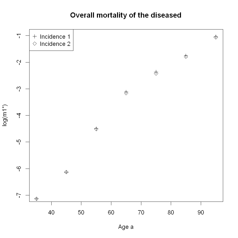
Figure 2 shows the overall mortality m1,iℓ⋆​(t,a)subscriptsuperscriptπ‘šβ‹†1subscriptπ‘–β„“π‘‘π‘Žm^{\star}_{1,i_{\ell}}(t,a) in year t=1𝑑1t=1 for the different incidences iβ„“,β„“=1,2,formulae-sequencesubscript𝑖ℓℓ12i_{\ell},\ell=1,2, over the age aπ‘Ža. The values have been calculated by Equation (10) using Romberg’s rule for integration. For ages below 50 the values m1,iℓ⋆​(t,a)subscriptsuperscriptπ‘šβ‹†1subscriptπ‘–β„“π‘‘π‘Žm^{\star}_{1,i_{\ell}}(t,a) rather agree, but diverge for ages between 50 and 80. For higher ages, the difference between m1,i1⋆subscriptsuperscriptπ‘šβ‹†1subscript𝑖1m^{\star}_{1,i_{1}} and m1,i2⋆subscriptsuperscriptπ‘šβ‹†1subscript𝑖2m^{\star}_{1,i_{2}} decreases again.

Refer to caption
Figure 2: Logarithm of the overall mortality of the diseased for two different incidence rates.

The reason for the differences can be seen in Figure 3, which depicts the duration distribution of the diseased persons C​(t=1,a)𝐢𝑑1π‘ŽC(t=1,a) for ages a=55,75,95.π‘Ž557595a=55,75,95.

Refer to caption
Figure 3: Duration distribution of the diseased persons for the different incidence rates iβ„“,β„“=1subscript𝑖ℓℓ1i_{\ell},~{}\ell=1 (crosses) and β„“=2β„“2\ell=2 (diamonds), at different ages: a=55π‘Ž55a=55 (left), a=75π‘Ž75a=75 (middle), a=95π‘Ž95a=95 (right).

From Figures 2 and 3 it becomes apparent that, although m1​(t,a,d)subscriptπ‘š1π‘‘π‘Žπ‘‘m_{1}(t,a,d) are the same for both diseases, the overall mortality m1⋆superscriptsubscriptπ‘š1⋆m_{1}^{\star} depends on the duration distribution of the diseased persons, which in turn depends on the incidence.

5 Discussion

This work generalizes the results of the previous articles [2] and [4] for the illness-death model as shown in Figure 1. In contrast to the previous articles, we do not need the assumption that the mortality of the diseased persons is independent from the duration of the disease. The modification that arises from possible duration dependence is the introduction of a measure for the mortality of the diseased persons, the overall mortality m1⋆.subscriptsuperscriptπ‘šβ‹†1m^{\star}_{1}. We have shown that m1⋆subscriptsuperscriptπ‘šβ‹†1m^{\star}_{1} depends on the duration distribution of the diseased persons, which in turn is a consequence of the incidence rate. With respect to the aim of deriving the age-specific incidence from prevalence data, this seems to be a drawback. However, if the duration distribution of the diseased persons is known, then the calculation of m1⋆subscriptsuperscriptπ‘šβ‹†1m^{\star}_{1} does not impose a problem. The request for having knowledge about the duration distribution is not unusual. It arises from the fundamental demand of epidemiology that the sample population (in a survey) should be a representative subset of the target population. Given that the duration distribution is known, calculation of m1⋆subscriptsuperscriptπ‘šβ‹†1m^{\star}_{1} from the duration dependent mortality m1subscriptπ‘š1m_{1} is possible. Another way of obtaining m1⋆superscriptsubscriptπ‘š1⋆m_{1}^{\star} is surveying it directly in an epidemiological study. If the sample population is representative for the target population – this means also representative with respect to the duration distribution – m1⋆superscriptsubscriptπ‘š1⋆m_{1}^{\star} may be obtained from standard survival analysis if the duration dependency is ignored. In this way, the overall mortality m1⋆subscriptsuperscriptπ‘šβ‹†1m^{\star}_{1} is an easily accessible epidemiological measure.

If, furthermore, the mortality m0subscriptπ‘š0m_{0} of the healthy, or at least the general mortality m=p​m1⋆+(1βˆ’p)​m0π‘šπ‘subscriptsuperscriptπ‘šβ‹†11𝑝subscriptπ‘š0m=p\,m^{\star}_{1}+(1-p)\,m_{0} is known, then Equation (9) can be used to obtain the incidence rate i𝑖i.

References

  • [1] Bernatsky S, Boivin JF, Joseph L et al (2006). Mortality in systemic lupus erythematosus. Arthritis Rheum 54(8): 2550-7.
  • [2] Brinks R (2011). A new method for deriving incidence rates from prevalence data and its application to dementia in Germany. arXiv:1112.2720
  • [3] Brinks R (2012). On characteristics of an ordinary differential equation and a related inverse problem in epidemiology. arXiv:1208.5476
  • [4] Brinks R (2012). On the age-, time- and migration dependent dynamics of diseases. arXiv:1209.1371
  • [5] Carstensen B, Kristensen JK, Ottosen P, Borch-Johnsen K (2008). The Danish National Diabetes Register: trends in incidence, prevalence and mortality. Diabetologia 51 (12):2187-96.
  • [6] Federal Statistical Office of Germany (2009). 12. Population Projection [12. Koordinierte BevΓΆlkerungsvorausberechnung] http://www.destatis.de, last access August 29th, 2013
  • [7] Hens N, Aerts M, Faes C et al (2010). Seventy-five years of estimating the force of infection from current status data. Epidemiol Infect 138(6):802-12.
  • [8] Keiding N (1991). Age-specific incidence and prevalence: a statistical perspective. J Royal Stat Soc A 154:371-412.
  • [9] Polyanin AD, Zaitsev VF, Moussiaux A (2000). Handbook of first order partial differential equations, Taylor & Francis, London
  • [10] Rait G, Walters K, Bottomly C et al (2010). Survival of people with clinical diagnosis of dementia in primary care: cohort study. BMJ 341:c3584.