What do observations of the Lyman $\alpha$ fraction tell us about reionization?

Abstract

An appealing approach for studying the reionization history of the Universe is to measure the redshift evolution of the Lyman $\alpha$ (Ly$\alpha$) fraction, the percentage of Lyman-break selected galaxies that emit appreciably in the Ly$\alpha$ line. This fraction is expected to fall-off towards high redshift as the intergalactic medium becomes significantly neutral, and the galaxies’ Ly$\alpha$ emission is progressively attenuated. Intriguingly, early measurements with this technique suggest a strong drop in the Ly$\alpha$ fraction near $z\sim 7$. Previous work concluded that this requires a surprisingly neutral intergalactic medium – with neutral hydrogen filling more than 50 per cent of the volume of the Universe – at this redshift. We model the evolving Ly$\alpha$ fraction using cosmological simulations of the reionization process. Before reionization completes, the simulated Ly$\alpha$ fraction has large spatial fluctuations owing to the inhomogeneity of reionization. Since existing measurements of the Ly$\alpha$ fraction span relatively small regions on the sky, and sample these regions only sparsely, they may by chance probe mostly galaxies with above average Ly$\alpha$ attenuation. We find that this sample variance is not exceedingly large for existing surveys, but that it does somewhat mitigate the required neutral fraction at $z\sim 7$. Quantitatively, in a fiducial model calibrated to match measurements after reionization, we find that current $z=7$ observations require a volume-averaged neutral fraction of $\langle x_{\rm HI}\rangle\geq 0.05$ at 95 per cent confidence level. Hence, we find that the $z\sim 7$ Ly$\alpha$ fraction measurements do likely probe the Universe before reionization completes but that they do not require a very large neutral fraction.

1 Introduction

Recent studies have identified large samples of Ly$\alpha$ emitting galaxies (LAEs) back to $z\sim 7$ (e.g. Hu et al. 2010; Ouchi et al. 2010; Kashikawa et al. 2011). In addition to providing insight into the properties of early galaxy populations, these surveys can be used to probe the ionization state of the surrounding intergalactic medium (IGM) and the reionization history of the Universe. In particular, the Ly$\alpha$ optical depth in a significantly neutral IGM is so large that even the red side of a Ly$\alpha$ emission line should be attenuated by absorption in the damping wing of the line (Miralda-Escude 1998). This is, in turn, expected to lead to a decline in the abundance of observable LAEs as the Universe becomes significantly neutral. Indeed, Kashikawa et al. (2006) found evidence for a decline in the abundance of LAEs between $z=5.7$ and $6.5$ from observations in the Subaru Deep Field (SDF). Recent work has started to extend these measurements all the way out to $z=7.7$ (e.g. Clément et al. 2012); this study finds no LAE candidates, possibly indicating a further drop in the abundance of LAEs from $z=6.5$ to $7.7$.

The declining LAE abundance may result if these observations are, in fact, probing into the Epoch of Reionization (EoR) when the IGM is significantly neutral, but the existence of a decline (e.g. Hibon et al. 2010, 2011, 2012; Tilvi et al. 2010; Krug et al. 2012), its statistical significance (Ouchi et al. 2010) and the interpretation of the measurements (e.g. Dijkstra et al. 2006) are all still debated. One main challenge here is to isolate the part of the evolution in the LAE abundance that arises from changes in the ionization state of the IGM. The LAE abundance itself will, undoubtedly, grow with time as a result of the hierarchical growth of the underlying LAE host halo population. Furthermore, the intrinsic properties of the LAE populations should also evolve with time. Evolution in the dust content, the structure of the interstellar medium, and the strength and prevalence of large scale outflows can all impact the escape of Ly$\alpha$ photons from galaxies, and the observable abundance of the LAE populations.

In recent work, Stark et al. (2010) proposed an approach that partly circumvents concerns about intrinsic evolution in the underlying galaxy populations. The Stark et al. (2010) method uses the Lyman-break selection technique to find populations of galaxies at the redshift of interest, taking advantage of that technique’s power in efficiently finding many galaxies within a given redshift range. Then, follow-up spectroscopy is done to determine which of those Lyman break galaxies (LBGs) have strong enough Ly$\alpha$ emission to be classified as LAEs. Since reionization should produce little to no effect on the observation of LBGs, but Ly$\alpha$ emission is attenuated by neutral hydrogen, the fraction of the LBGs that are also LAEs should decrease as the IGM becomes significantly neutral. With this technique, evolution in the abundance of the underlying population of star-forming galaxies ‘divides out’. Evolution in the Ly$\alpha$ fraction induced by changes in the intrinsic LAE properties can be extrapolated from lower redshift measurements of this fraction at $z\leq 5$ or so, which clearly probe the post-reionization epoch. Moreover, the spectroscopic samples obtained in this approach allow one to search for spectroscopic signatures of intrinsic evolution in the LAEs’ properties.

Several groups have recently applied this method for the first time; our focus here will be on the theoretical interpretation of these new measurements. First, Stark et al. (2010, 2011) measured the Ly$\alpha$ fraction ($f_{Ly\alpha}$) in several redshift bins, centred around $z=4,5$, and $6$. The Universe should be completely ionized in this case, at least in the former two redshift bins, and so this measurement describes the redshift evolution in the intrinsic LAE properties towards high redshift. These authors find evidence that $f_{Ly\alpha}$ increases steadily from $z=4-6$. They explain this trend by noting that dust levels in these galaxies tend to decrease with increasing redshift; this should likely facilitate the escape of Ly$\alpha$ photons and so $f_{Ly\alpha}$ should grow with increasing redshift. Having noted this trend, they make predictions for $f_{Ly\alpha}$ at $z\sim$ 7, assuming there is no evolution in the ionized fraction. A lower measurement of $f_{Ly\alpha}$ than predicted would hence suggest that $z\sim 7$ observations are probing the significantly neutral era.

Very recently, several groups have extended these measurements out to $z\sim 7$, including Schenker et al. (2012), Pentericci et al. (2011), Ono et al. (2012) and Caruana et al. (2012). As we discuss in more detail subsequently, both Schenker et al. (2012) and Pentericci et al. (2011) see evidence for a decline in $f_{Ly\alpha}$ near $z\sim 7$. Both Ono et al.’s and Caruana et al.’s results are consistent with little evolution from Stark et al. (2011)’s lower redshift measurements to within their error bars. Although these measurements are still in their infancy, and come from $\leq 50$ LBGs in total, the strong decline seems to suggest that the IGM is surprisingly neutral at $z\sim 7$. In particular, Pentericci et al. (2011) argue that the low $f_{Ly\alpha}$ indicated by their $z\sim 7$ measurement requires a volume-averaged neutral fraction of $\langle x_{\rm HI}\rangle\geq 0.6$. Schenker et al. (2012) quote a fairly similar constraint, although somewhat more tentatively.

Interestingly, the large neutral fractions suggested by this test are surprising given other constraints on reionization. In particular, the relatively large optical depth to Thomson scattering implied by Wilkinson Microwave Anisotropy Probe (WMAP) observations (Larson et al. 2011) and the low emissivity – only a few ionizing photons per atom per Hubble time at $z\sim 5$ – inferred from the mean transmission in the Ly$\alpha$ forest after reionization (Miralda-Escude 2003; Bolton and Haehnelt 2007) suggest that reionization is a fairly prolonged and extended process. Furthermore, the absence of prominent Gunn–Peterson absorption troughs in $z\leq 6$ quasar spectra (Fan et al. 2006) is commonly taken to imply that the IGM is completely ionized by $z\leq 6$, a mere $175$ Myr after the time period probed by the $z=7$ Ly$\alpha$ fraction measurements. Hence the Ly$\alpha$ fraction test results, when combined with $z\leq 6$ quasar absorption spectra measurements, are hard to reconcile with other observational constraints – as well as theoretical models for the redshift evolution of the ionized fraction – which all prefer a more extended reionization epoch. One possibility is that reionization is sufficiently inhomogeneous to allow transmission through the Ly$\alpha$ forest before the process completes (Lidz et al. 2007; Mesinger 2010), potentially relaxing the requirement that reionization needs to complete by $z\geq 6$ (McGreer et al. 2011). Nevertheless, collectively current constraints on reionization prefer a significantly higher ‘mid-point’ redshift at which 50 per cent of the volume of the IGM is neutral, $z_{50}$. For example, Kuhlen and Faucher-Giguère (2012) (see also Pritchard et al. 2010) combine measurements of the Thomson scattering optical depth, high-redshift LBG luminosity functions, and measurements from the post-reionization Ly$\alpha$ forest, finding that the preferred redshift at which $\langle x_{\rm HI}\rangle=0.5$ is $z_{50}=10$ for a variety of models.

However, as we look back into the EoR we expect both the average abundance of LAEs to decrease and for there to be increasingly large spatial fluctuations in the abundance of observable LAEs (Furlanetto et al. 2006; McQuinn et al. 2007a; Mesinger and Furlanetto 2008; Jensen et al. 2013). This should result from the patchiness of the reionization process: LAEs that reside at the edge of ionized regions, or in small ionized bubbles, will have significant damping wing absorption from nearby neutral hydrogen, while those at the centre of large ionized bubbles will be less attenuated. Ultimately, measuring these spatial variations is a very promising approach for isolating the impact of the IGM and studying reionization, with existing data already providing some interesting constraints (McQuinn et al. 2007a; Ouchi et al. 2010). Presently, the important point is that these fluctuations imply that one must survey a rather large region on the sky to obtain a representative sample of the Ly$\alpha$ fraction. Perhaps existing $z\sim 7$ measurements in fact probe later stages in reionization than previously inferred, but are sampling regions on the sky with above average attenuation and correspondingly lower than average Ly$\alpha$ fractions. Here we set out to explore this sample variance effect, quantify its impact on existing measurements, and to understand the requirements for future surveys to mitigate its impact.

The significance of the observed drops in the Ly$\alpha$ fraction also depends on the relationship between LAE and LBGs; therefore, we examine a variety of models in an attempt to span some of the uncertainties in the properties of the galaxies themselves. We use simulations to explore the effects of small fields of view and various models for LBG luminosity and Ly$\alpha$ emission on $f_{Ly\alpha}$ and, thus, what can be confidently said about the ionized fraction of the Universe.

Throughout this paper, we assume a $\Lambda$ cold dark matter ($\Lambda$CDM) model with $n_{\rm{s}}=1$, $\sigma_{8}=0.8$, $\Omega_{\rm{m}}=0.27$, $\Omega_{\Lambda}=0.73$, $\Omega_{\rm{b}}=0.046$ and $h=0.7$. These parameters are broadly consistent with recent results from the Planck collaboration (Ade et al. 2013).

2 Observations

First, we describe all of the current $z\sim 7$ Ly$\alpha$ fraction measurements. We subsequently compare these measurements with theoretical models. The main properties of the current observations are summarized in Table 1.

Pentericci et al. (2011) describe observations they obtained over three fields of view: the Great Observatories Origins Deep Surey (GOODS)-South field (Giavalisco et al. 2004), the New Technology Telescope Deep Field (NTTDF; Arnouts et al. (1999); Fontana et al. (2000)) and the BDF-4 field (Lehnert and Bremer 2003). Altogether, these fields span 200 arcmin² [roughly 700 (Mpc $h^{-1}$)²]. Within these fields, they did follow-up spectroscopy on galaxies that were selected as $z$-dropouts. As we will discuss, in practice their spectroscopic sample probes the Ly$\alpha$ attenuation across only a fraction of these full fields-of-view. Although these results are summarized and combined by Pentericci et al. (2011), they also published the initial measurements in stages. In Fontana et al. (2010), they report their observations on GOOD-S. In Vanzella et al. (2011), they do the same for galaxies in BDF-4. Finally, in Pentericci et al. (2011), they discuss their observations of NTTDF. In these fields combined, they found 20 LBGs, two of which had strong enough Ly$\alpha$ emission for them qualify at LAEs.

They bin these galaxies based both on ultraviolet (UV) magnitude and on the rest-frame equivalent widths of the Ly$\alpha$ lines, REWs. Since none of the faint galaxies ($-20.25<M_{UV}<-18.75$) that they observe has strong Ly$\alpha$ emission, for the faint case they are only able to put upper limits on $f_{Ly\alpha}$. For the galaxies with stronger Ly$\alpha$ emission (REW $>$ 55 Å), their results are consistent within error bars with the projections from lower redshifts by Stark et al. (2011). It is only for the weaker, but UV bright $(M_{\rm{UV}}<-20.25)$, LAEs (REW $>$ 25 Å) that they directly detect a significant drop.

Schenker et al. (2012) do spectroscopic follow-up on LBGs with z $>$ 6.3 observed in the Hubble Space Telescope (HST) Early Release Science (ERS) field by Hathi et al. (2010) and McLure et al. (2011), 36.5 arcmin² [119 (Mpc $h^{-1}$)²]. In addition to the eight galaxies they observed in ERS, they also included 11 galaxies drawn from a variety of other surveys. From this sample of 19 galaxies, they found two that were LAEs. In order to boost their sample size, they also considered galaxies studied by Fontana et al. (2010) in their calculation of $f_{Ly\alpha}$. Note that since Fontana et al. (2010) is part of the sample sets from both Pentericci et al. (2011) and Schenker et al. (2012), these two sets of observations are not completely independent. Fontana et al. (2010) detected seven LBGs none of which was clearly LAEs. Thus, Schenker et al. (2012) worked from a total sample of 26 LBGs, two of which they identified as LAEs.

Combining these data sets and taking into account the various limits of the observations, they find that $f_{Ly\alpha}$ for the brighter galaxies ($-21.75<M_{\rm{UV}}<-20.25$) is consistent with the lower redshift measurements. It is only for the faint galaxies ($-20.25<M_{UV}<-18.75$) that they see a significant drop.

Ono et al. (2012) observed the SDF and GOODS-N, a total of 1568 arcmin² [roughly 5100 (Mpc $h^{-1}$)²]. However, their survey is much shallower than either Schenker et al. (2012) or Pentericci et al. (2011), only observing down to $y\simeq$ 26.0 mag ($M_{UV}=-20.9$). Because of this shallowness, even though they are observing a relatively large area, they only identified 22 $z$-dropout candidates (Ouchi et al. 2009). From that sample, they took spectroscopic observations of 11 of them; three of those they identified as LAEs. Their study only goes as deep as the brightest of two $M_{UV}$ bins ($-21.75<M_{UV}<-20.25$). In that bin, their results are consistent with the projections of Stark et al. (2011) from lower redshifts.

Caruana et al. (2012) did spectroscopy for five $z$-band dropouts ($z\sim 7$) found in the Hubble Ultra Deep Field, 11 arcmin² [36 (Mpc $h^{-1}$)²], selected from earlier surveys. They observed no Ly$\alpha$ emission from the $z$-band dropouts, and, thus, only placed upper limits on the $f_{Ly\alpha}$ at $z\sim 7$; their upper limits are consistent with the projections from lower redshifts (Stark et al. 2011).

One might wonder, for all of these surveys, about the presence of low redshift interlopers. If the fraction of low redshift interlopers is larger near $z\sim 7$ than at lower redshifts, one might erroneously infer a drop-off in the Ly$\alpha$ fraction. For instance, in the simplest version of the Lyman break selection technique a lower redshift red galaxy may be mistaken for a higher redshift LBG. However, these groups have used a variety of techniques to ensure that the samples are truly from a redshift near $z\sim 7$, preferring to discard those galaxies that are likely, but not definitively, at the redshift of interest in order to obtain an uncontaminated sample. In particular, Pentericci et al. (2011), as discussed in Castellano et al. (2010), use multiple filters and a number of colour selection criteria, to ensure that low-redshift interlopers are excluded. Similarly, the sample used by Ono et al. (2012), drawn from Ouchi et al. (2009), applies a variety of colour cuts to only select high redshift galaxies. Schenker et al. (2012) derive their main sample from McLure et al. (2011). McLure et al. (2011) fit the photometric redshifts of all potential candidates and required the ones that they retained to have both statistically acceptable solutions for $z>6$ and to exclude lower redshift solutions at the 95 per cent confidence level. Based on all of these techniques, interloper contamination appears not to be a significant worry.

Since only Pentericci et al. (2011) and Schenker et al. (2012) report significant decreases in $f_{Ly\alpha}$, the rest of the paper will focus on their observations. As detailed in Table 1, it is notable that the typical comoving dimension of all but the shallower Ono et al. (2012) survey is $\sim 10$ Mpc $h^{-1}$. This scale is comparable to the size of the ionized regions during much of the EoR (see e.g. McQuinn et al. 2007b), suggesting that sample variance may be significant on these scales. Furthermore, as we detail subsequently, the LBGs identified for follow-up spectroscopy in these fields only sparsely sample sub regions of the full field, and so the surveys do not, in fact, sample Ly$\alpha$ attenuation across the entire field of view.

Table 1: Summary of published measurements of $f_{Ly\alpha}$

Field	Area	Shortest side	Limiting mag ($y$ band)	Faint1		Brightb		Sourcec
				LBGs	LAEs	LBGs	LAEs
Pentericci et al. (2011)
BDF-4	$\sim$ 50 arcmin2	13.6 Mpc $h^{-1}$	26.5	1	0	5	2	Vanzella et al. (2011); Pentericci et al. (2011)
GOODS-S	$\sim$ 90 arcmin2	13.6 Mpc $h^{-1}$	26.7	1	0	6	0	Fontana et al. (2010)
NTTDF	$\sim$ 50 arcmin2	13.6 Mpc $h^{-1}$	26.5	0	0	7	0	Pentericci et al. (2011)
Schenker et al. (2012)
GOODS-S	$\sim$ 90 arcmin2	13.6 Mpc $h^{-1}$	26.7	1	0	6	0	Fontana et al. (2010)
ERS	36.5 arcmin2	7.7 Mpc $h^{-1}$	27.26	8	0	0	0	Schenker et al. (2012)
Other fieldsc	–	–	–	7	2	4	0	Schenker et al. (2012)
Ono et al. (2012)
GOODS-N	$\sim$ 150 arcmin2	18.1 Mpc $h^{-1}$	26.0	0	0	1	1	Ono et al. (2012)
SDF	$\sim$ 1400 arcmin2	48.9 Mpc $h^{-1}$	26.0	0	0	7	2	Ono et al. (2012)
Caruana et al. (2012)
HUDF	$\sim$ 11 arcmin2	6.0 Mpc $h^{-1}$	–e	3	0	2	0	Caruana et al. (2012)
aFaint galaxies are ones with $-20.25<M_{UV}<-18.75$
bBright galaxies are ones with $-21.75<M_{UV}<-20.25$
cMay not have originally observed these galaxies, but did the spectroscopic follow up and reported which ones had Ly$\alpha$ emission
d Schenker et al. (2012) included several galaxies from a variety of other surveys and fields in their spectroscopic sample. These have been grouped together here.
e Caruana et al. (2012) did spectroscopic follow up on galaxies drawn from several surveys. Thus, there is no consistent y-band limiting magnitude.
Summary of observations for the main papers we are discussing. The Fontana et al. (2010) sample is included in both the observations of Pentericci et al. (2011) and Schenker et al. (2012). This is because both groups used that data in their calculation of $f_{Ly\alpha}$. Galaxies were only counted as LAEs if their Ly$\alpha$ emission was greater than some minimum threshold (usually an equivalent width threshold of 25 Å). In compiling this table, summaries in Ono et al. (2012) were essential.

3 Method

Next we describe the various ingredients that enter into our simulated models of the Ly$\alpha$ fraction. Our calculations start from the reionization simulations of McQuinn et al. (2007a); these simulations provide realizations of the inhomogeneous ionization field and surrounding neutral gas, which in turn modulate the observable abundance of the simulated LAEs. In post-processing steps, we further populate simulated dark matter haloes with LBGs and LAEs, finally attenuating the LAEs based on the simulated neutral hydrogen distribution. A completely self-consistent approach would vary the reionization history jointly with variations in the properties of the LBGs and LAEs, but our post-processing approach offers far greater flexibility for exploring a wide range of models. In addition, most of the ionizing photons are likely generated by much fainter, yet more abundant, sources than the LBGs that are detected directly (thus far) and so the ionization history is somewhat decoupled from the LBG properties relevant here. Our philosophy for modelling the LAEs is to focus our attention on the impact of reionization and its spatial inhomogeneity. As a result, we presently ignore the complexities of the Ly$\alpha$ line transfer internal to the galaxies themselves; we will comment on their possible impact on our main conclusions.

3.1 Reionization simulations

The reionization simulations used in our analysis are described in McQuinn et al. (2007b, a); here we mention only a few pertinent details. These simulations start from a $1024^{3}$ particle, $130$ comoving Mpc $h^{-1}$ dark matter simulation run with gadget-2 (Springel 2005) and treat the radiative transfer of ionizing photons in a post-processing step. The calculation resolves host haloes down to $\sim 10^{10}M\odot$, and so the simulation directly captures the likely host haloes of both LBGs and LAEs (smaller mass haloes host ionizing sources and are added into the simulation as described in McQuinn et al. (2007a)). We adopt the fiducial model of these authors in which each halo above the atomic cooling mass (on the order of $M\sim 10^{8}M\odot$, Barkana and Loeb 2001) hosts a source with an ionizing luminosity that is directly proportional to its halo mass. We consider simulation outputs with a range of ionized fractions, $\langle x_{i}\rangle$, in effort to explore how the Ly$\alpha$ fraction and its spatial variations evolve throughout reionization. In each case, we take the host haloes from a simulation output at $z=6.9$, very close to the redshift of interest for the current Ly$\alpha$ fraction measurements. In the fiducial model of McQuinn et al. (2007a) studied here, the volume-averaged ionization fraction is $\langle x_{i}\rangle=0.82$ at this redshift. In practice, when we explore smaller ionized fractions, we use slightly higher redshift outputs of the ionization field in the same model. This approximation was also adopted in McQuinn et al. (2007a) and should be adequate since – at fixed $\langle x_{i}\rangle$ – the properties of the ionization field depend little on the precise redshift at which the ionized fraction is reached (tests of this are given in McQuinn et al. 2007b).

3.2 LBG model

The next step in our model is to populate the simulated dark matter haloes with LBGs. Here we follow the simple approach described in Stark et al. (2007). In this model, the star formation rate, $\dot{M}_{\star}$, is connected to the halo mass, $M_{\rm halo}$, by

$$\dot{M}_{\star}=\frac{f_{\star}(\Omega_{\rm{b}}/\Omega_{\rm{m}})M_{\rm{halo}}}{t_{\rm{LT}}},$$ (1)

where $f_{\star}$ is the efficiency at which baryons are converted into stars and $t_{\rm{LT}}$ is the time-scale for star formation, which is itself the product of the star formation duty cycle ($\epsilon_{\rm{DC}}$) and the age of the Universe which – in the high-$z$ approximation – is $t(z)=2/(3H(z))$. We assume here that stars form at a constant rate in the haloes that are actively forming stars. We adopt Stark et al. (2007)’s best-fitting values of $f_{*}=0.16$ and $\epsilon_{\rm{DC}}=0.25$, for LBGs at $z\simeq 6$. We further assume the conversion from star formation rate to UV luminosity (at a rest-frame wavelength of $\lambda=1500\mbox{ \AA}$) given in Madau et al. (1998):

$$L_{1500}=8.0\times 10^{27}\frac{\rm{erg}}{\rm{Hz\ s}}\left[\frac{\dot{M}_{\star}}{1M\odot/\rm{yr}}\right].$$ (2)

The conversion factor here assumes a Saltpeter initial mass function and solar metallicity, but we do not expect our results to be sensitive to the precise number here. In the simple model described here, $\epsilon_{\rm{DC}}$ also gives the fraction of host haloes that are UV luminous at any given time. However, we find that the observed number density of LBGs at $z\sim 7$ from Bouwens et al. (2011) is better reproduced if instead $1/6$th of simulated dark matter haloes host LBGs with the above luminosity. In practice we randomly select $1/6$th of our dark matter haloes as active LBG hosts and give them UV luminosities according to the above formulas (with $\epsilon_{\rm{DC}}=0.25$). This also allows us to reproduce the bias factor found from large samples of LBGs (Overzier et al. 2006). The assumption here of a one-to-one relation between UV luminosity and host halo mass for the active hosts is undoubtedly a simplification, but we have experimented with adding a $20$ per cent scatter to the UV luminosity–halo mass relation above and found little difference in our results.

3.3 Properties of the LAEs

Next, we give each LBG a random amount of Ly$\alpha$ emission, as characterized by the REW of each emission line. Our main interest is to explore the impact of inhomogeneous damping-wing absorption on the Ly$\alpha$ fraction, and so we do not attempt a detailed modelling of each emission line. In addition to the complex impact of the Ly$\alpha$ line transfer internal to each galaxy, the resulting line will be modified by resonant absorption within the IGM (in addition to the damping wing absorption that we do explicitly model). It is sometimes assumed that each emission line is symmetric upon leaving the galaxy, and that the blue side of each line is removed by resonant absorption in the surrounding IGM while the red side is fully transmitted. The reality is of course more complicated, and even the resonant absorption in the IGM may have a wide range of effects depending on the strength of large-scale infall motions towards LAE host haloes (which can lead to resonant absorption on the red side of the line), the local photoionization state of the gas, outflows, and other factors (see e.g. Santos 2004; Dijkstra et al. 2007; Zheng et al. 2010; Verhamme et al. 2012; Yajima et al. 2012; Duval et al. 2013). We will assume that these variations are captured by drawing the REW of each LBG from a random distribution. We will refer to this loosely as the intrinsic REW, and that the observed REW results from simply multiplying this intrinsic REW by a damping wing attenuation factor described below. In this sense, our intrinsic REW is intended to include resonant absorption from the IGM, and we implicitly assume that this distribution does not vary strongly from $z\sim 6$ to $z\sim 7$. We additionally neglect any spatial variations – induced by e.g., large scale infall motions – in the intrinsic REW distribution.

As in Dijkstra et al. (2011), we draw an REW for each simulated galaxy from an exponential distribution, $P(\rm{REW})=\rm{exp}[-REW/REW_{c}]/REW_{c}$. This exponential model provides a good fit to the distribution of REWs found in lower redshift galaxies (Gronwall et al. 2007; Blanc et al. 2011). We further allow the REW to be either uncorrelated, correlated, or anti-correlated with the UV luminosity of each simulated LBG. In our fiducial model, the REW and UV luminosity are anti correlated since this trend appears to best reproduce existing observations. In order to produce REW distributions that are anti correlated with UV luminosity, we draw REWs from the exponential distribution (with $\rm{REW_{c}}=125\mbox{ \AA}$ in our fiducial model), and place them into various REW bins that are then populated with LBGs according to their UV luminosity. Specifically, we divide REWs into 10 bins based on width: the first bin is from 0 to 32 Å, the second from 32 to 110 Å and the remaining eight are 80 Å wide. The LBGs are then divided into 10 bins based on UV luminosity, and the most luminous galaxies are randomly assigned REWs from the first (smallest REW) REW bin, the next most luminous from the first and second bins, and so forth, until all the LBGs have REWs. Although the details of this procedure are somewhat arbitrary, it matches both the observed values of $f_{Ly\alpha}$ at $z\sim 6$ (for both UV bright and UV faint sources), as well as the correlation coefficient, $\rho$, between REW and UV luminosity. This is defined as

$$\rho=\frac{\sum\limits_{i=1}^{n}(\rm{REW_{i}}-\overline{\rm{REW}})(L_{i}-\overline{L})}{\sqrt{\sum\limits_{i=1}^{n}(\rm{REW}_{i}-\overline{\rm{REW}})^{2}}\sqrt{\sum\limits_{i=1}^{n}(L_{i}-\overline{L})^{2}}}.$$ (3)

The sum here is over the LAEs in the observed or simulated sample, with $n$ LAEs in total, $\rm{REW_{i}}$ denotes the rest frame equivalent width of the $i$th LAE in the sample, $L_{i}$ is the UV luminosity of the $i$th LAE, while $\overline{\rm{REW}}$ and $\overline{L}$ denote the sample-averaged rest frame equivalent width and UV luminosity, respectively. The correlation coefficient in our fiducial model is $\rho=-0.23$, while from fig. 12 of Stark et al. (2010) we infer $\rho=-0.41$; since the variance of the observational estimate is likely still sizeable, we consider this simple model to be broadly consistent with observations.

This negative correlation model is also physically plausible, as discussed in §4.2. Of course, our fiducial description of this correlation is only a toy model. Nevertheless, we believe that it captures the relevant features of the lower redshift observations, and, thus, should be a useful guide as we consider the $f_{Ly\alpha}$ measurements.

In addition to our fiducial model, we discuss three other models that seem both physically plausible and show a diversity of results: (1) the REWs are assigned randomly; (2) there is a weak positive correlation between the REW and continuum luminosity of the galaxy and (3) there is a weak negative correlation between the REW and the continuum luminosity of the galaxy – weaker than in our fiducial case. For the second and third cases, the REWs are assigned in a fashion similar to that in our fiducial case, except the galaxies, and REWs, are only divided into three bins, not 10. Thus, the correlation is weaker than in the fiducial case. For the weak positive correlation, the correlation coefficient is $\rho=0.10$; for the weak negative correlation, $\rho=-0.11$. While these models are unlikely to perfectly capture the relationship between LAEs and LBGs, they suffice to explore how our results depend on the precise relationship between LBGs and LAEs.

3.4 Attenuated LAE emission and mock surveys

The intrinsic emission from each LAE is then attenuated according to the simulated distribution of neutral hydrogen. We do this following McQuinn et al. (2007a) and Mesinger and Furlanetto (2008). Specifically, we shoot lines of sight through the simulation box towards each LAE and calculate the total damping wing contribution to the Ly$\alpha$ optical depth, summing over intervening neutral patches. As in this previous work, we calculate the damping wing optical depth $\tau_{\rm{DW}}$ (according to e.g., equation 1 of Mesinger and Furlanetto 2008) only at the centre of each emission line, i.e. at an observed wavelength of $\lambda_{\rm{obs}}=\lambda_{\alpha}(1+z_{\rm{s}})$ for a source at redshift $z_{\rm{s}}$, with $\lambda_{\alpha}=1215.67\mbox{ \AA}$ denoting the rest-frame line centre of the Ly$\alpha$ line. We ignore the impact of peculiar velocities and neglect any redshift evolution in the properties of the ionization field across our simulation box – we use snapshots of the simulated ionization field at fixed redshift. Calculating the optical depth at the centre of each line, rather than the full profile, should be a good approximate indicator of which sources will be attenuated below observational REW cut-offs (see McQuinn et al. 2007a for a discussion and tests). The ‘observed’ REW of each simulated LBG is then an attenuated version of the initial intrinsic REW according to $\rm{REW}_{\rm{obs}}=\rm{e}^{-\tau_{\rm{DW}}}\rm{REW}$.

Armed with galaxy positions, UV luminosities and observed REWs, we produce mock realizations of the Schenker et al. (2012) and Pentericci et al. (2011) observations, and measure their statistical properties. We slice the simulation cube into strips with the perpendicular dimensions mimicking the geometry and field of view of the observations. In order to approximately mimic the survey window functions in the redshift direction, we assume each strip has a length of 100 comoving Mpc $h^{-1}$. We adopt this value based on the estimated redshift distribution of $z$’-band dropouts in Ouchi et al. (2009) (their fig. 6), which those authors determined from the SDF and GOODS-N fields. For simplicity, we assume a top-hat window function and find that a top-hat of width 100 Mpc $h^{-1}$ reproduces the area under the redshift distribution curve of Ouchi et al. (2009) and so use this width throughout. While all three of these surveys (Ouchi et al. 2009; Pentericci et al. 2011; Schenker et al. 2012) use slightly different filters, they all peak at roughly the same wavelength and Ouchi et al. (2009)’s have the largest full width at half maximum (FWHM). Thus, this should be a reasonable approximation, although it may slightly overestimate the depth of the field.

Within these strips, we then select the galaxies that would be observable to the two groups, based on the limiting magnitudes and REW limits they reported (see Table 1). One subtlety here is that the galaxies observed by both groups are not distributed across their entire fields. This likely occurs partly because the LBGs are clustered, and partly because their efficiency for detecting LBGs and performing spectroscopic follow-up is not uniform across each field. Because of the latter effect, we may underestimate the sample variance if we draw the simulated LBGs from the full field of view. To roughly mimic this, we draw our LBGs from randomly placed cylinders with diameters matching the largest separation between galaxies in each set of observations: 9.99 Mpc $h^{-1}$ for Schenker et al. (2012) and 8.04 Mpc $h^{-1}$ for Pentericci et al. (2011). We only consider observable galaxies that fall within each cylinder, effectively limiting the size of the observed fields and making them still closer to the size of the ionized bubbles in the simulation.

Furthermore, comparing to the $z\sim 7$ LBG luminosity function from (Bouwens et al. 2011), it is clear that the existing measurements perform spectroscopic follow-up on only a small fraction of the total number of LBGs expected in each survey field. This likely owes mostly to the expense of the spectroscopic follow-up observations. However, this implies that the Ly$\alpha$ fraction measurements only sparsely sample the Ly$\alpha$ attenuation across the entire field-of-view, and enhances the sample variance effect. To mimic this, in each mock survey we randomly select LBGs to match the precise number spectroscopically observed, and consider the Ly$\alpha$ emission and attenuation around only these galaxies. In the case of Schenker et al. (2012)’s ERS field, they actually do not observe any bright LBGs. To loosely consider this case – which will turn out to be less constraining – we randomly select four simulated LBGs, which matches their bright sample in the other fields and also corresponds to the number one would expect based on the size of their field of view and the follow-up capabilities in Pentericci et al. (2011).

One caveat here is that our simulation does not capture Fourier modes that are larger than our simulation box size (130 comoving Mpc $h^{-1}$), and so the sample variance we estimate is only a lower bound. We do not expect the ‘missing variance’ to be large, however. Although the full fields of view of some of the existing surveys correspond to a decent fraction of our simulation volume (see Table 1), the effective volume probed by the observations is significantly smaller, as a result of the sparse sampling discussed previously. In addition, it is important to note that our simulation box size is large compared to the size of the ionized regions during most of the reionization epoch, and so it does suffice to capture a representative sample of the ionization field.

Since both teams did follow up spectroscopy on already identified LBGs, we look for Ly$\alpha$ emission in the selected LBGs that is strong enough to exceed the observed REW cuts. The field-to-field fluctuations in $f_{Ly\alpha}$ arise from both the sample variance we aim to study and from discreteness fluctuations. In our model, the latter arise because the REW of the Ly$\alpha$ emission from each LBG is drawn from a random distribution. This scatter is, of course, non-vanishing even in the absence of reionization-induced inhomogeneities, and moreover, it is already included in the error budget of the existing measurements (while the sample variance contribution has not been included). Hence we must separate the discreteness and sample variance contributions to the simulated variance in order to avoid double counting the discreteness component. To do this, we keep track of which LBGs fluctuate above and below the observational REW cuts as a result of an upward or downward fluctuation in the IGM attenuation. Some LBGs in the simulated sample are observable as LAEs only because of downward fluctuations in the IGM attenuation, while some are pulled out of the LAE sample because of upward fluctuations in the IGM attenuation. Finally, in some cases – depending on the LBG’s intrinsic REW and IGM attenuation – the IGM attenuation does not impact the LBG’s observability as an LAE. Monitoring which LBGs are pulled into or out of the sample owing to fluctuations in the IGM attenuation allows us to measure the scatter in $f_{Ly\alpha}$ arising from sample variance alone.

Schenker et al. (2012) combine observations from a variety of surveys. Their observations focus on galaxies selected from an LBG survey on the ERS field. To increase their sample size, Schenker et al. (2012) include observations from Fontana et al. (2010) and several other LBGs from a variety of fields in their analysis. Since Fontana et al. (2010) is included in Pentericci et al. (2011)’s analysis and the other LBGs were not all detected in well defined drop-out surveys of the corresponding fields, we only model the observations of the ERS field of view when we analyse Schenker’s results.

Pentericci et al. (2011) observed with four pointings of the High Acuity Wide Field K-Band Imager (HAWK-I; two in GOODS-S, one at BDF-4 and one at NTTDF). Although the two fields in GOOD-S are next to each other, for ease of calculation we treated each pointing as independent, and scaled the confidence regions accordingly. This may lead us to underestimate the sample variance from these observations slightly.

4 Discussion

4.1 Is a large neutral fraction required?

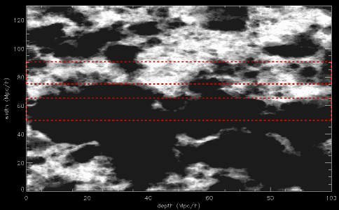
Figure 1: A slice through the simulation cube for an output with a volume-averaged ionization fraction of $\langle x_{\rm{i}}\rangle=0.82$. The slice is averaged over one (perpendicular to the line of sight) dimension of the ERS field of view. Clouds of neutral gas are shown in grey-scale; the white areas being completely neutral. The dashed lines mark two potential mock ERS observations. The significant difference between these two fields illustrates that small regions on the sky may not provide representative samples of the overall average ionization state of the IGM.

Before we present a detailed comparison between the Ly$\alpha$ fraction measurements and our simulated models and explore their implications for understanding reionization, a qualitative illustration of the main effect discussed here may be helpful. This is provided by Fig.  1, which shows a representative slice through the simulation volume, when the volume-averaged ionization fraction is $\langle x_{\rm{i}}\rangle=0.82$. The dimension into and out of the page has been averaged over the size of an ERS field. The two red regions show example mock survey volumes that have the same size as an ERS field. Clearly the top field is fairly well covered by intervening neutral hydrogen, although it is still has patches of ionized hydrogen. On the other hand, the bottom cylinder is almost entirely clear of neutral hydrogen. LBGs residing in the top cylinder will be much more attenuated than in the bottom panel.

Quantitatively, in the faint UV luminosity bin of Schenker et al. (2012), the simulated $f_{Ly\alpha}$ in the first simulated field is $f_{Ly\alpha}=0.30$, while the Ly$\alpha$ fraction is almost twice as large in the second simulated field, $f_{Ly\alpha}=0.58$. These numbers can be compared to the average across the entire simulation volume at this neutral fraction, which is $f_{Ly\alpha}=0.51$. Using our fiducial model and supposing (incorrectly) that these fractions are representative, one would infer an ionized fraction of $\langle x_{\rm{i}}\rangle=0.54$ for the first field, compared to $\langle x_{\rm{i}}\rangle=1.0$ for the second field. Neither inference correctly returns the true ionized fraction of the field, $\langle x_{\rm{i}}\rangle=0.82$. This suggests that a rather large area survey is indeed required to obtain representative measurements of the Ly$\alpha$ fraction. Perhaps the existing fields are more like the top cylinder, and the LBGs in these fields suffer above average attenuation. Assuming a survey like the top cylinder is representative of the volume averaged neutral fraction could clearly bias one’s inferences of the neutral fraction. The chance of obtaining a biased estimate of the neutral fraction is enhanced if spectroscopic follow-up is done on only a few LBGs – effectively, a sparse sampling of each survey region – as is often the case for the existing measurements.

With this intuitive understanding, we turn to a more detailed comparison with the observations. Schenker et al. (2012) report a decline in $f_{Ly\alpha}$ at $z$ $\sim$ 7. This decline is particularly pronounced when compared to their observed $f_{Ly\alpha}$ values at lower redshifts. For $4<z<6$, they report an increase in the Ly$\alpha$ fraction with increasing redshift (Stark et al. 2011). At $z$ $\sim$ 7, $f_{Ly\alpha}$ is lower than the projected trend and lower than measured at $z$ $\sim$ 6. This decline suggests that that the observations may be probing into the EoR. Using Monte Carlo simulations of their full data sample, Schenker et al. (2012) conclude that in order to explain their results they require an ionized hydrogen fraction of at most $\langle x_{\rm{i}}\rangle\leq 0.51$.

Note that the low redshift measurements ($4<z<6$) come mainly from observations of the GOODS fields, both North and South. Some additional galaxies from other sources are also included. Altogether, Stark et al. (2011) observed 351 $B$-dropouts, 151 $V$-dropouts, and 67 i’-dropouts. Given the large sky coverage of these surveys, sample variance should not be a significant source of error for the low-redshift measurements. However, the same may not be true at higher redshift where the measurements come from smaller fields of view. In addition, if the high-redshift measurements probe into the EoR, this should enhance the sample variance as we will describe.

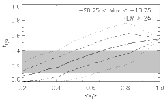
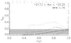
Figure 2: Comparison between mock Ly$\alpha$ fraction ($f_{Ly\alpha}$) measurements and the observations of Schenker et al. (2012), as a function of the volume-averaged ionization fraction, $\langle x_{\rm{i}}\rangle$. The solid lines show the average value of $f_{Ly\alpha}$ across the simulation volume in our fiducial model, while the dotted and dashed lines indicate the field-to-field spread in the simulated Ly$\alpha$ fraction, i.e. the sample variance. The dashed lines enclose the values of $f_{Ly\alpha}$ for 68 per cent of the mock ERS fields, while the dotted lines enclose 95 per cent of the simulated fields. The shaded regions show the 68 per cent confidence interval reported by Schenker et al. (2012) (which neglect the sample variance contribution). The horizontal line near the centre of the shaded bands gives their best-fitting value for the Ly$\alpha$ fraction. The top panel is for the UV faint bin of Schenker et al. (2012), while the bottom panel is for the UV bright bin.

In Fig. 2 we show simulated Ly$\alpha$ fractions for mock surveys mimicking the $z\sim 7$ measurements of Schenker et al. (2012) for the ERS field. In particular, we plot the average Ly$\alpha$ fraction across the entire simulation box (solid line), as well as 68 per cent (dotted lines) and 95 per cent (dashed lines) confidence intervals, as a function of the volume-averaged ionization fraction ($\langle x_{\rm{i}}\rangle$) in the models. The lines reflect the field-to-field variance (i.e. the sample variance) in the simulated $f_{Ly\alpha}$ values. The probability distribution of simulated $f_{Ly\alpha}$ values is somewhat non-Gaussian, and so we account for this in determining the confidence intervals. In order to compare with Schenker et al. (2012) we divide the simulated LBGs into UV bright ($-21.75<M_{UV}<-20.25$) (bottom panel) and UV faint ($-20.25<M_{UV}<-18.75$) (top panel) bins. The shaded region in each panel gives the allowed range in $f_{Ly\alpha}$ at 68 per cent confidence reported by Schenker et al. (2012), while the horizontal line shows their best-fitting $f_{Ly\alpha}$ value. In calculating the 68 per cent confidence range, Schenker et al. (2012) include LBGs from several fields. As discussed earlier, we only calculate the sample variance for the ERS field. The sample variance may thus be slightly overestimated when compared to the rest of the error budget. The shaded region neglects the sample variance contribution, and so a better estimate of the total error budget is the quadrature sum of the shaded regions and the dashed lines.

Focusing first on the UV faint bin (top panel), the first conclusion we draw from this comparison is that the best-fitting ionized fraction is indeed $\langle x_{\rm{i}}\rangle\approx 0.5$. This is consistent with the conclusions of Schenker et al. (2012). Note, however, that Schenker et al. (2012) infer the neutral fraction from the same McQuinn et al. (2007a) simulations used here, and so their constraint is not independent of the results here, although our present calculations adopt a different model for the LAE/LBG populations. The next conclusion to draw from the top panel is that the spread from sample variance is generally comparable to (although a little smaller than) the reported error budget, and so it is not in fact negligible, aside from the fully ionized case where it vanishes in this model. Here the sample variance describes spatial variations in the damping wing attenuation, which vanish in the fully ionized model. In reality, spatial variations in the resonant absorption likely lead to additional contributions, neglected here, which would make the sample variance non-vanishing in the fully ionized case. Accounting for sample variance somewhat reduces the neutral fraction required by these observations; for instance an $\langle x_{\rm{i}}\rangle\approx 0.85$ model is just outside of the allowed 68 per cent confidence range.

The bottom panel shows that the UV bright case is still easier to accommodate in a highly ionized IGM, at least in our fiducial LAE model. In this case, Schenker et al. (2012) found little evidence for redshift evolution. Since our fiducial model is constructed to give a lower $f_{Ly\alpha}$ fraction for UV bright LBGs after reionization, the Ly$\alpha$ fraction remains small at $z\sim 7$ in a highly ionized IGM. In fact, since the UV bright galaxies tend to have smaller intrinsic REWs in our fiducial model, these galaxies are particularly susceptible to attenuation: that Schenker et al. (2012) detect some Ly$\alpha$ emission from UV bright galaxies in this model then actually slightly disfavours more neutral models. At the 68 per cent confidence level, $\langle x_{\rm{i}}\rangle\approx 0.42$ or smaller is disfavoured. The relatively small number of LBGs spectroscopically followed up in each field (only four) contributes to the size of the error bars. Recall that our sampling of four model galaxies here is somewhat arbitrary, as Schenker et al. (2012) did not in fact follow up any bright LBGs in the ERS field. Further, the trend of LAE fraction with ionization fraction depends somewhat on our particular model for the anti-correlation between intrinsic REW and UV luminosity, as we describe in §4.2.

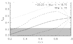
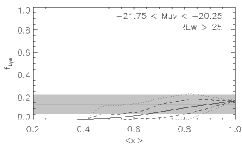
Figure 3: Comparison between mock Ly$\alpha$ fraction ($f_{Ly\alpha}$) measurements and the observations of Pentericci et al. (2011) as a function of the volume-averaged ionization fraction, $\langle x_{\rm{i}}\rangle$. This is similar to Fig. 2 expect here the shaded bands are the measurements from Pentericci et al. (2011), with UV faint measurements in the top panel, and UV bright ones in the bottom panel. Likewise, the simulated observations in this figure mimic those of Pentericci et al. (2011).

Similarly, we can compare our mock Pentericci et al. (2011) observations with their actual measurements. This is shown in Fig. 3. Their survey is not as deep as Schenker et al. (2012), but covers a larger area on the sky. In the faint UV luminosity bin, they search for Ly$\alpha$ emission around two LBGs (see Table 1), and find no significant Ly$\alpha$ emission from either galaxy. This allows them to place only an upper limit on $f_{Ly\alpha}$ in this luminosity bin. Their quoted upper limit none the less implies a drop-off towards high redshift in $f_{Ly\alpha}$, when compared to the lower redshift measurements of Stark et al. (2011). However, the sample variance in our simulated samples is significant. In particular, the top panel shows that the upper limit on $f_{Ly\alpha}$ translates into a lower limit on the neutral fraction of $0.2$ at the 68 per cent confidence level. The spread in $f_{Ly\alpha}$ values is large because only two LBGs are studied spectroscopically, and there are large variations in the amount of damping wing attenuation suffered by these two LBGs, depending on whether they reside towards the centre of large ionized regions, at the edge of an ionized region, or in the centre of a smaller ionized bubble.

For the UV bright galaxies, they do detect some Ly$\alpha$ emission; in this luminosity bin their Ly$\alpha$ fraction is lower for small REW ($\rm{REW}>25\mbox{ \AA}$) lines than expected from extrapolating the lower redshift Stark et al. (2011) measurements out to $z\sim 7$. However, in our fiducial model the decline in the Ly$\alpha$ fraction for the UV bright sample is not especially constraining. As discussed previously, these sources tend to have smaller intrinsic REWs, and so even a small amount of attenuation from the IGM attenuates them out of the observable sample. Indeed the bottom panel of Fig. 3 shows that the Ly$\alpha$ fraction in the UV bright Pentericci et al. (2011) bin is compatible with a fully ionized universe in our fiducial model. As with the case of Schenker et al. (2012), this bin actually (slightly) disfavours too large a neutral fraction, $\langle x_{\rm{HI}}\rangle<0.52$ at the 68 per cent confidence level. Once the neutral fractions is less than $0.4$, $f_{Ly\alpha}$ is consistent with zero; thus, that Pentericci et al. (2011) observe any Ly$\alpha$ disfavours a highly neutral universe.

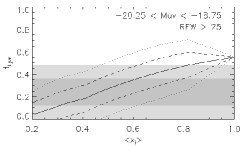
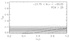
Figure 4: Confidence intervals on $f_{Ly\alpha}$ from combining the measurements of Schenker et al. (2012) and Pentericci et al. (2011). These constraints are compared to our fiducial model, as a function of $\langle x_{\rm{i}}\rangle$. Similar to Figs 2 and 3, except here the results reflect the constraints from combining the separate Ly$\alpha$ fraction measurements. The shaded regions reflect the combined reported errors, while the lines indicate the simulated average and sample variance contributions to the error budget. The top panel is for the UV faint luminosity bin, while the bottom panel is for the UV bright bin.

Of course, that both Pentericci et al. (2011) and Schenker et al. (2012) observe evidence for a drop in $f_{Ly\alpha}$ near $z\sim 7$ strengthens the case that these observations probe back into the EoR. In order to quantify this, we combine the probability distributions for the separate observations shown in Figs 2 and 3. The results of this calculation are shown in Fig 4. Here the shaded regions show the 68 and 95 per cent confidence intervals after combining the two measurements, assuming that the reported error distributions obey Gaussian statistics. For the combined UV faint case, we used directly the combined uncertainty calculated in Ono et al. (2012) which took into account that Fontana et al. (2010) was included in the calculations of both Pentericci et al. (2011) and Schenker et al. (2012). As before, the lines show the sample variance contributions calculated from our simulated models (and not included in the shaded error budgets).

We do not consider the observations of Ono et al. (2012) or Caruana et al. (2012) here since we do not expect them to have a significant effect on the combined constraints. While Ono et al. (2012) observed a large field, their survey was fairly shallow and focused on a small number of galaxies–only following up on 11 galaxies in the bright bin. Since the faint galaxies place the greatest constraints on the ionized fraction in our fiducial model, a shallow survey, focusing on the bright galaxies, is unlikely to increase the constraints. Further, Ono et al. (2012)’s observations are consistent with the increasing trend in $f_{Ly\alpha}$ seen in Stark et al. (2011); Ono et al. (2012) do not see a drop in $f_{Ly\alpha}$ at $z\sim 7$. Together, these characteristics of their observations, mean that not considering their observations does not significantly affect our results. Further, by only observing 11 galaxies, Ono et al. (2012) greatly reduce their survey’s effective volume. Of course, a deeper survey, with more galaxies sampling the entire large field, would greatly reduce the effects of sample variance and could place significant constraints on the ionized fraction.

Caruana et al. (2012), on the other hand, focused on an extremely small field of view. The size of their field makes them particularly vulnerable to sample variance. Their observations are consistent with the trend from Stark et al. (2011). Thus, their observations would not place any further constraint on the sample variance.

The constraints in the combined case follow the trends found for each separate survey, but the overall significance is somewhat tightened. As before, the low Ly$\alpha$ fraction in the UV bright case is consistent with a fully ionized model. The UV faint case does, however, prefer a partly neutral IGM, but a very large neutral fraction is not required. For example, a model with $\langle x_{i}\rangle\sim 0.9$ lies within the 95 per cent confidence range.

4.2 Model dependance

It is also interesting to explore how the simulated Ly$\alpha$ fractions depend on the underlying model for the Ly$\alpha$ emission from LBGs. In particular, our fiducial model assumes that the intrinsic Ly$\alpha$ REW is anti correlated with UV luminosity. A variety of studies seem to support this relationship. At $z$ $\simeq$ 3, Shapley et al. (2003) report an increase in the mean REW with fainter luminosity. Stark et al. (2010) extend this out to higher redshift; for their sample of LBGs with Ly$\alpha$ emission at $3\la z\la 6$, they find that the largest REWs tend to correlate with fainter UV continuum magnitudes. These observations are supported by a host of others (Ando et al. 2006; Ouchi et al. 2008; Vanzella et al. 2009; Balestra et al. 2010) that suggest that among the brightest sources, large REWs are scarce. Such a correlation has a plausible explanation; the fainter galaxies may be less dusty than their brighter counterparts, allowing more of the Ly$\alpha$ emission to be transmitted.

While this model does seem to match observations, there is still not widespread agreement on this point, see, for instance, Kornei et al. (2010). For LBGs at $z\sim 3$, Kornei et al. (2010) do not see a significant correlation between continuum luminosity and Ly$\alpha$ emission. Nilsson et al. (2009) argue that a flux or magnitude-limited survey, like the ones cited above, will generally observe both fewer instances of strong Ly$\alpha$ emission and fewer instances of bright LBGs since those are both rare. Thus, in order to conclude that continuum luminosity and Ly$\alpha$ REWs are anti-correlated one would need very large sample sizes, on the order of 1000 LBGs with measured REWs. In addition, note that our fiducial model was tuned to match the observations of Stark et al. (2011) in a fully ionized universe. However, there is still some uncertainty in the post-reionization Ly$\alpha$ fractions, even for UV bright sources. For example, Curtis-Lake et al. (2012) find a $z\sim 6$ Ly$\alpha$ fraction that is roughly two times as large as that of Stark et al. (2011) for UV bright sources, and comparable to that of the UV fainter sources from Stark et al. (2011).

$\begin{array}[]{ccc}\includegraphics[scale={0.28}]{combo_anti_faint.eps}\par\includegraphics[scale={0.28}]{combo_1_faint.eps}\par\includegraphics[scale={0.28}]{combo_cor_faint.eps}\\ \includegraphics[scale={0.28}]{combo_anti_bright.eps}\par\includegraphics[scale={0.28}]{combo_1_bright.eps}\par\includegraphics[scale={0.28}]{combo_cor_bright.eps}\par\end{array}$

Figure 5: Dependence of $f_{Ly\alpha}$ on the LAE model. Similar to Fig. 4, but here we consider three different models for assigning Ly$\alpha$ REWs to LBGs. Left: there is a weak negative correlation between the continuum luminosities and the Ly$\alpha$ REWs; the fainter galaxies have stronger Ly$\alpha$ emission, but the trend is less strong than in our fiducial model. Middle: the Ly$\alpha$ REWs are assigned randomly to the LBGs, following the distribution in Dijkstra et al. (2011). Right: there is a weak positive correlation between the continuum luminosities and the Ly$\alpha$ REWs; the brighter galaxies have stronger Ly$\alpha$ emission. The top panels are for UV faint bins, while the bottom panels show UV bright LBGs.

Given the uncertainties in the relationship between LBGs and their intrinsic Ly$\alpha$ emission, we generate combined constraints along the lines of Fig. 4 for three additional LAE models. These additional models are described in §3.3 and correspond to cases with: a weaker negative correlation between intrinsic REW and UV luminosity than in our fiducial model (with $\rho=-0.11$ from Equation 3 compared to $\rho=-0.23$ in our fiducial model); a model where REW and UV luminosity are uncorrelated and a model with a weak positive correlation ($\rho=0.10$).

The combined constraints in these additional models are shown in Fig. 5. It is reassuring that the results in the UV faint bin appear only weakly dependent on the underlying model for Ly$\alpha$ emission from LBGs. The UV bright case is, on the other hand, quite sensitive to the underlying LAE model. In particular, in these models the UV bright Ly$\alpha$ fractions are intrinsically larger than in our fiducial case, and so significant attenuation is required to explain the lower Ly$\alpha$ fractions measured in the high UV luminosity bin. However, the same qualitative behaviour is expected in the post-reionization Universe, and so each of these models is in conflict with the post-reionization ($z\sim 4-6$) measurements of Stark et al. (2011) which do show a significant drop in the Ly$\alpha$ fraction from UV faint to UV bright LBGs.

Our model does not consider the effects of galactic winds on Ly$\alpha$ emission. Backscattering of Ly$\alpha$ emission off of the far side of a galactic outflow can promote the escape of Ly$\alpha$ photons by shifting them redward of line centre, and strong winds may therefore make Ly$\alpha$ emission more visible even in a highly neutral universe. Thus, explaining the drop in $f_{Ly\alpha}$ reported in these surveys would require a more neutral universe than we have argued (Dijkstra et al. 2011), strengthening the conclusions of Schenker et al. (2012) and Pentericci et al. (2011). However, while strong winds are observed from LBGs at $z\sim 3$ (e.g. Shapley et al. 2003), the outflow speed – and hence the redshift imparted to Ly$\alpha$ photons – may be substantially smaller around the smaller mass galaxies typical near $z\sim 7$. It is presently unclear how prevalent strong winds are from $z\sim 7$ LBGs.

Clearly, a better understanding of the relationship between LBGs and LAEs should help in interpreting current and future Ly$\alpha$ fraction measurements. Along these lines, Dayal and Ferrara (2012) have simulated LBGs and LAEs at $z$ $\sim$ 6, 7 and 8. They conclude that LAEs are a diverse subset of LBGs. While the faintest LBGs do not have Ly$\alpha$ emission, LAEs are found distributed throughout all other categories of LBGs. Similarly, Forero-Romero et al. (2012) model the relationship between LBGS and LAEs in the range $5\leq z\leq 7$, concluding that, in order to match the observations of Stark et al. (2011), the Ly$\alpha$ escape fraction must be inversely correlated with galaxy luminosity. Further observational and theoretical work should help strengthen our understanding of the precise relationship between these two galaxy populations.

5 Conclusions

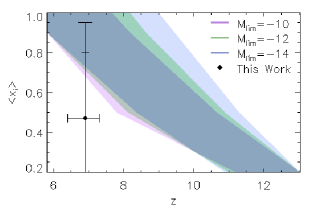
Figure 6: The reionization history inferred from a variety of observations. The shaded band shows constraints on the ionization fraction as a function of redshift from Kuhlen and Faucher-Giguère (2012), which come from combining WMAP-7 measurements of the optical depth to Thomson scattering, the intensity of the UV background inferred from the $z\sim$ 2-5 Ly$\alpha$ forest, and measurements of the UV galaxy luminosity function at high redshift. The luminosity functions are extrapolated down to faint luminosities; the different shaded bands show the dependence on the limiting UV magnitude ($M_{\rm{lim}}$) out to which this extrapolation is carried out. The point with error bars shows the constraint we infer from the Ly$\alpha$ fraction measurements of Schenker et al. (2012) and Pentericci et al. (2011). The lower vertical error bar shows the 68 per cent confidence interval, while the upper vertical error bar shows the 95 per cent confidence interval. The horizontal error bar gives the redshift uncertainty for the LBGs used in these measurements.

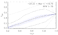
Figure 7: The impact of improved sampling of the Pentericci et al. (2011) fields on the sample variance error. Pentericci et al. (2011) looked for Ly$\alpha$ emission from two faint LBGs. This leads to the large sample variance, shown in the black dashed and dotted lines, at 68 and 95 per cent, respectively (identical to the lines in the top panel of Fig. 3). The blue dashed and dotted lines show that the sample variance would dramatically shrink if a survey was done to search for Ly$\alpha$ emission from all of the LBGs in their fields.

In order to summarize our findings and put them in the larger context of our current understanding of the EoR, we use the results of Fig. 4 to compute the likelihood function for $\langle x_{\rm{i}}\rangle(z\sim 7)$ given the results of both Schenker et al. (2012) and Pentericci et al. (2011). Fig. 6 shows the resulting 68 and 95 per cent confidence regions for $\langle x_{\rm{i}}\rangle$, as compared to constraints from Kuhlen and Faucher-Giguère (2012), which combine recent WMAP-7 measurements of the Thomson scattering optical depth, along with observations of the $z\sim 2-5$ Ly$\alpha$ forest, and UV galaxy luminosity function measurements. Although the central value of $\langle x_{\rm{i}}\rangle(z\sim 7)$ we infer from the $f_{Ly\alpha}$ observations is outside of the range implied by the other measurements, accounting for sample variance and other sources of uncertainty in the $f_{Ly\alpha}$ measurements, we find that these various observations are in fact in broad agreement with each other. Interestingly, we conclude that a fully ionized IGM is disfavoured by the $f_{Ly\alpha}$ measurements, although a highly neutral IGM ($\langle x_{\rm{i}}\rangle\leq\sim 0.5$) is not required. Taken together with spectroscopic observations of a $z=7.1$ quasar from Mortlock et al. (2011), the case that existing measurements probe into the EoR is strengthening.

It is also interesting to note that recent and improved measurements of the UV galaxy luminosity function from the Ultra Deep Field (UDF) survey and Cosmic Assembly Near-Infrared Deep Extragalactic Survey (CANDELS) favour somewhat later reionization than in the Kuhlen and Faucher-Giguère (2012) analysis (Oesch et al. 2013; Robertson et al. 2013). For instance, extrapolating the measured luminosity functions down to $M_{\rm UV}<-13$, Robertson et al. (2013) favours $z\sim 7.5$ for the redshift at which the Universe is $50$ per cent neutral by volume (see their Fig. 5). These results are more easily harmonized with the preferred (central) value of $\langle x_{\rm{i}}\rangle(z\sim 7)$ inferred from the $f_{Ly\alpha}$ observations.

We also find that the constraints from the Ly$\alpha$ fraction measurements depend somewhat on the model relating the properties of the LBGs and LAEs. In our fiducial model (shown here in Fig. 6), the intrinsic REW of Ly$\alpha$ emission from LBGs is anti-correlated with UV luminosity. In models without this anti correlation, the lower Ly$\alpha$ fractions among UV bright galaxies at both $z\sim 7$ and at lower redshifts ($z\sim 4-6$) are hard to understand.

Bolton and Haehnelt (2013) recently pointed out another effect that may also help reconcile the Ly$\alpha$ fraction measurements with other constraints on reionization. These authors suggest that the observed drops in the Ly$\alpha$ fraction towards high redshift may be driven mostly by strong evolution in the number of dense, optically thick absorbers in the vicinity of the observed LBGs, rather than reflecting prominent changes in the ionization state of the diffuse IGM. This effect would not be well captured in the simulations used in our analysis, since these dense absorbers are notoriously difficult to resolve in large volume reionization simulations. This effect would also, however, presumably show large field-to-field variations, similar to the spatial variations in the attenuation from the diffuse gas studied here. More detailed models will likely be necessary to disentangle the relative impact of optically thick, circumgalactic absorbers and the more diffuse IGM considered here.

More importantly, the prospects for improved observations are very good, and especially tantalizing given the current hints that $z\sim 7$ observations may probe into the EoR. Larger and deeper surveys for LBGs and LAEs should help clarify the interpretation of current observations. In particular, as shown in Fig. 7, observing down to $M_{UV}=-18.75$ over an area as large as that observed by Pentericci et al. (2011) would be enough to greatly reduce the effects of sample variance. Fully sampling such an area, however, would mean spectroscopically observing on the order of 100s of LBGs, looking for Ly$\alpha$ emission. However, even just sampling five galaxies per field (20 galaxies total) is enough to ‘fill in’ the sparse sampling and reduce the sample variance by a factor of 2. Alternatively, the use of narrow-band filters to select the LBGs that are also LAEs should make observing 100s feasible.

The spatial fluctuations in the Ly$\alpha$ fraction studied here are presently a nuisance; however, they should ultimately provide a very interesting and distinctive signature of reionization, provided they can be mapped out over large volumes of the Universe. Mapping these fluctuations will require both larger fields of view and more fully sampled fields than currently available. This should, nonetheless, be possible using upcoming observations from the Hyper Suprime-Cam on the Subaru telescope, which will observe LAEs out to $z=7.3$ over more than $5$ deg².

6 Acknowledgements

We thank Matt McQuinn for providing the reionization simulations used in our analysis and for comments on a draft. JT and AL were supported by NASA grant NNX12AC97G.

References

- Ade et al. (2013) Ade, P. et al.: 2013, ArXiv e-prints
- Ando et al. (2006) Ando, M., Ohta, K., Iwata, I., et al.: 2006, ApJL 645, L9
- Arnouts et al. (1999) Arnouts, S., D’Odorico, S. Cristiani, S., Zaggia, S., Fontana, A., and Giallongo, E.: 1999, A&A 341, 641
- Balestra et al. (2010) Balestra, I., Mainieri, V., Popesso, P., et al.: 2010, A&A 512, A12
- Barkana and Loeb (2001) Barkana, R. and Loeb, A.: 2001, Phys. Rep. 349, 125
- Becker and Bolton (2013) Becker, G. D. and Bolton, J. S.: 2013, ArXiv e-prints
- Blanc et al. (2011) Blanc, G. A., Adams, J. J., Gebhardt, K., et al.: 2011, ApJ 736, 31