Distribution function approach to redshift space distortions. Part V: perturbation theory applied to dark matter halos

Zvonimir Vlah    Uroš Seljak    Teppei Okumura    Vincent Desjacques
Abstract

Numerical simulations show that redshift space distortions (RSD) introduce strong scale dependence in the power spectra of halos, with ten percent deviations relative to linear theory predictions even on relatively large scales (k<0.1h/Mpc𝑘0.1𝑀𝑝𝑐k<0.1h/Mpc) and even in the absence of satellites (which induce Fingers-of-God, FoG, effects). If unmodeled these effects prevent one from extracting cosmological information from RSD surveys. In this paper we use Eulerian perturbation theory (PT) and Eulerian halo biasing model and apply it to the distribution function approach to RSD, in which RSD is decomposed into several correlators of density weighted velocity moments. We model each of these correlators using PT and compare the results to simulations over a wide range of halo masses and redshifts. We find that with an introduction of a physically motivated halo biasing, and using dark matter power spectra from simulations, we can reproduce the simulation results at a percent level on scales up to k0.15h/Mpcsimilar-to𝑘0.15𝑀𝑝𝑐k\sim 0.15h/Mpc at z=0𝑧0z=0, without the need to have free FoG parameters in the model.

1 Introduction

Galaxy clustering surveys are one of the most important venues of extracting cosmological information today. The reason is that by measuring the 3 dimensional distribution of galaxies we can in principle relate it to the 3 dimensional distribution of the underlying dark matter, and dark matter distribution is sensitive to many of the cosmological parameters. Growth of dark matter structures in time also provides important constraints on the models, such as the nature and amount of dark energy in the Universe. Since galaxies are not the perfect tracers of dark matter, their clustering is biased relative to the dark matter. This means that galaxy surveys cannot determine the rate of growth of structure unless this biasing is determined. Fortunately, galaxy redshift surveys provide additional information, because the observed redshift is a sum of the radial distance to the galaxy and its peculiar velocity (Doppler shift). Galaxies are expected to follow the same gravitational potential as the dark matter and thus are expected to have the same velocity (in a large-scale average at least). This leads to a clustering strength that depends on the angle between the galaxy pairs and the line of sight, which is referred to as redshift space distortions (RSD). In linear theory this can be easily related to the dark matter clustering [1, 2]. These distortions thus make the galaxy clustering in redshift space more complex, but at the same time provide an opportunity to extract important information on the dark matter clustering directly from the redshift surveys. To what extent this is possible is still a matter of debate: there are significant nonlinear effects that spoil this picture, once one goes beyond the very large scales. The goal of this paper is to explore these nonlinear effects using analytic modeling.

Velocity induced RSD are usually decomposed into two competing effects: anisotropies along the line of sight due to the large coherent motion, so called Kaiser effect, and random motions in virialized objects, known as the Finger-of-God effect (FoG) [3]. Because of the large coherent motions the RSD anisotropies offer a unique way to measure growth rate of structure formation [4], and also can provide tests of dark energy models and general relativity [5, 6, 7, 8, 9, 10, 11, 12]. If good understanding of the nonlinear effects were achieved, RSD would be the most powerful technique for these studies because of the fact that redshift surveys provide 3-dimensional information, while other methods, such as weak lensing, only provide projected 2-dimensional information (or slightly more if the so-called tomographic information is used [13]).

In the past many studies have been performed investigating these nonlinear effects [14, 15, 16, 17, 18, 19, 20, 21]. Some of these methods use analysis and modelling based on perturbation theory (for overview see [22, 23]), but none attempt to rely entirely on perturbation theory to explain all of the effects. Instead, they use ansatzes with free parameters, so that if the ansatz are accurate one can model the effects accurately. Separately, there have been many approaches trying to improve perturbation methods and to increase their ranges of validity [24, 25, 26, 27, 28, 29, 30, 31, 32, 33, 34, 35, 36]. Going beyond the dark matter modelling to the dark matter halos and galaxies introduces another layer of complication. Dark matter halos are biased relative to the underling dark matter and in order to describe them biasing models have to be introduced. Many models have been introduced in order to describe this relation [37, 38, 39, 40, 41], and some have also been included in RSD studies [42, 43, 44, 45, 46, 47, 48, 49, 50].

Distribution function approach to modelling the RSD has recently been developed [51] as a systematic way to study the nonlinear effects in RSD, by decomposing RSD effects into a series of mass-weighted powers of velocity correlators. This approach has been utilized for the dark matter case using the N-body simulations [52] and each of the constituent terms has been modeled in PT [53]. This model naturally generalizes to the dark matter halos, which have been analyzed using the N-body simulations in [54]. It has been shown that halo clustering in redshift space has a scale dependence relative to linear theory that is stronger than in real space. The goal of this paper is to explain this using Eulerian perturbation theory (PT) modelling applied to the halos. We adopt the local Eulerian biasing model as a tool to connect the underlying dark matter distribution to the halos, but we also explore effects beyond the local biasing model, probing the effects of higher order nonlocal terms [39, 55].

The paper is organized as follows: we begin in Sec.2 by generalizing the distribution function approach to RSD for dark matter halo case. We then introduce the biasing model, and applying it to model the velocity moment correlators. In Sec. 3 we collect all the modelled terms and investigate the total RSD power spectrum results. We compare the results to the multipoles in Fourier space as well as in configuration space. Results are compared to the N-body simulation measurements presented in [54].

For this work, flat ΛΛ\LambdaCDM model is assumed Ωm=0.279subscriptΩm0.279\Omega_{\rm m}=0.279, ΩΛ=0.721subscriptΩΛ0.721\Omega_{\Lambda}=0.721, Ωb/Ωm=0.165subscriptΩbsubscriptΩm0.165\Omega_{\rm b}/\Omega_{\rm m}=0.165, h=0.7010.701h=0.701, ns=0.96subscript𝑛𝑠0.96n_{s}=0.96, σ8=0.807subscript𝜎80.807\sigma_{8}=0.807. The primordial density field is generated using the matter transfer function by CAMB. The positions and velocities of all the dark matter halos are given at the redshifts z=0,0.509,0.989𝑧00.5090.989z=0,~{}0.509,~{}0.989, and 2.070, which are for simplicity quoted as z=𝑧absentz=0, 0.5, 1, and 2.

2 Redshift-space distortions from the distribution function

2.1 Definitions and starting equations

Following the recent work on phase space approach to redshift space distortions [51, 52, 54, 53], distribution function expansion developed for dark matter can be generalized to the dark matter halos. We can write for halo overdensity field in redshift space

δsh(k)=δh(k)+j=11j!(ik)j[(1+δh(x))uj(x)](k),subscriptsuperscript𝛿𝑠ksuperscript𝛿ksubscript𝑗11𝑗superscript𝑖subscript𝑘parallel-to𝑗delimited-[]1superscript𝛿xsubscriptsuperscript𝑢𝑗parallel-toxk\delta^{h}_{s}(\textbf{k})=\delta^{h}(\textbf{k})+\sum_{j=1}\frac{1}{j!}\left(\frac{ik_{\parallel}}{\mathcal{H}}\right)^{j}\mathcal{F}\left[\left(1+\delta^{h}(\textbf{x})\right)u^{j}_{\parallel}(\textbf{x})\right](\textbf{k}), (2.1)

where usubscript𝑢parallel-tou_{\parallel} is the halo velocity field projected along the line of sight, and ksubscript𝑘parallel-tok_{\parallel} projection of the Fourier mode along the line of sight direction. Also \mathcal{F} stands for the Fourier transformation defined in this paper as;

f~(k)=[f(x)](k)=d3xexp(ikx)f(x),~𝑓kdelimited-[]𝑓xksuperscript𝑑3𝑥exp𝑖kx𝑓x\displaystyle\tilde{f}(\textbf{k})=\mathcal{F}\left[f(\textbf{x})\right](\textbf{k})=\int{d^{3}x~{}\text{exp}(i\textbf{k}\cdot\textbf{x})f(\textbf{x})},
f(x)=1[f~(k)](x)d3k(2π)3exp(ikx)f~(k).𝑓xsuperscript1delimited-[]~𝑓kxsuperscript𝑑3𝑘superscript2𝜋3exp𝑖kx~𝑓k\displaystyle f(\textbf{x})=\mathcal{F}^{-1}\left[\tilde{f}(\textbf{k})\right](\textbf{x})\int{\frac{d^{3}k}{(2\pi)^{3}}~{}\text{exp}(-i\textbf{k}\cdot\textbf{x})\tilde{f}(\textbf{k})}. (2.2)

Using the halo filed expression we can define the dark matter halo-halo power spectrum in redshift-space

(2π)3Ps(hh)(k)δD(kk)=δsh(k)δsh(k).superscript2𝜋3subscriptsuperscript𝑃𝑠ksuperscript𝛿𝐷ksuperscriptkdelimited-⟨⟩subscriptsuperscript𝛿𝑠ksubscriptsuperscript𝛿absent𝑠superscriptk\displaystyle(2\pi)^{3}P^{(hh)}_{s}(\textbf{k})\delta^{D}(\textbf{k}-\textbf{k}^{\prime})=\left\langle\delta^{h}_{s}(\textbf{k})\delta^{*h}_{s}(\textbf{k}^{\prime})\right\rangle. (2.3)

Dark matter halos are considered to be biased tracers of the underlying dark matter. Identifying the correct biasing model has been proven to be a challenging task, and there is still a lot of ongoing work on this subject. In the standard local bias approach the halo field can be considered as a functional of the underlying dark matter density field δh[δ]superscript𝛿delimited-[]𝛿\delta^{h}[\delta]. In addition to the local relation of the constructed halo field and the underlying matter overdensity field one can also expect nonlocal effects ([38]). For example, in [39, 40, 55] effects of the tidal tensor biasing have been considered. In this paper we adopt the model presented in [55] where the only nonlocal term is due to the second order tidal tensor, which is added to the standard Taylor expansion of local bias, which we expand to 2nd order. We will see that the tidal tensor bias term does not play the crucial role in modeling the two point statistic of biased object as has already been shown in [40], but we will nevertheless keep the term in the following expressions. In addition, the third order nonlocal term may also play an important role in explaining the biasing effects in two point halo statistics studied in this paper. We will include this possibility here in a simplified model, deferring a more detailed analysis to a future paper. In addition to the nonlocal density contributions there are also potential velocity bias effects which, if present, might be important in modelling the halo velocity moments. This is a subject of ongoing studies using initial density peaks [56, 57]. Clear results from these studies are still to be determined and so we will not include this possibility here. Finally, there are also the effects of exclusion which were emphasized recently in [58]. We will include them in a simplified model.

We use Eulerian biasing model

δh(x)=b1δ(x)+b22(δ2(x)δ2)+bs2(s2(x)s2)+b36δ3(x),superscript𝛿xsubscript𝑏1𝛿xsubscript𝑏22superscript𝛿2xdelimited-⟨⟩superscript𝛿2subscript𝑏𝑠2superscript𝑠2xdelimited-⟨⟩superscript𝑠2subscript𝑏36superscript𝛿3x\delta^{h}(\textbf{x})=b_{1}\delta(\textbf{x})+\frac{b_{2}}{2}\left(\delta^{2}(\textbf{x})-\left\langle\delta^{2}\right\rangle\right)+\frac{b_{s}}{2}\left(s^{2}(\textbf{x})-\left\langle s^{2}\right\rangle\right)+\frac{b_{3}}{6}\delta^{3}(\textbf{x}), (2.4)

where δ𝛿\delta is underlying dark matter overdensity field, and bisubscript𝑏𝑖b_{i} are the coresponding bias parameters. We also add the nonlocal biasing term bssubscript𝑏𝑠b_{s} presented in [55], and more extensively studied in [39],

s2(k)=d3q(2π)3S(2)(q,kq)δ(q)δ(kq),S(2)(k,q)=(kq)2q2k213.formulae-sequencesuperscript𝑠2ksuperscript𝑑3𝑞superscript2𝜋3superscript𝑆2qkq𝛿q𝛿kqsuperscript𝑆2kqsuperscriptkq2superscript𝑞2superscript𝑘213s^{2}(\textbf{k})=\int{\frac{d^{3}q}{(2\pi)^{3}}S^{(2)}(\textbf{q},\textbf{k}-\textbf{q})\delta(\textbf{q})\delta(\textbf{k}-\textbf{q})},\qquad S^{(2)}(\textbf{k},\textbf{q})=\frac{(\textbf{k}\cdot\textbf{q})^{2}}{q^{2}k^{2}}-\frac{1}{3}. (2.5)

From now on we will use the abbreviations for the integrations of the convolution form

(UV)k=d3q(2π)3U(q)V(kq)=UqVkqsubscript𝑈𝑉ksuperscript𝑑3𝑞superscript2𝜋3𝑈q𝑉kqsubscript𝑈qsubscript𝑉kq\displaystyle(U\circ V)_{\textbf{k}}=\int{\frac{d^{3}q}{(2\pi)^{3}}U(\textbf{q})V(\textbf{k}-\textbf{q})}=U_{\textbf{q}}V_{\textbf{k}-\textbf{q}} (2.6)

in order to make following expressions shorter. To use this biasing model we need to preform Fourier transformation, which leads to

δkh=b1δk+b22δqδkq+bs2sk2+b36δqδqδkqq,subscriptsuperscript𝛿ksubscript𝑏1subscript𝛿ksubscript𝑏22subscript𝛿qsubscript𝛿kqsubscript𝑏𝑠2subscriptsuperscript𝑠2ksubscript𝑏36subscript𝛿qsubscript𝛿superscriptqsubscript𝛿kqsuperscriptq\delta^{h}_{\textbf{k}}=b_{1}\delta_{\textbf{k}}+\frac{b_{2}}{2}\delta_{\textbf{q}}\delta_{\textbf{k}-\textbf{q}}+\frac{b_{s}}{2}s^{2}_{\textbf{k}}+\frac{b_{3}}{6}\delta_{\textbf{q}}\delta_{\textbf{q}^{\prime}}\delta_{\textbf{k}-\textbf{q}-\textbf{q}^{\prime}}, (2.7)

and for the higher moments of phase space distribution function

TLh=TLh,(k)[1/ρ¯d3qfh(x,q)qL],T^{h}_{L}=T^{h,\parallel}_{L}(\textbf{k})\equiv\mathcal{F}\left[1/\bar{\rho}\int{d^{3}q~{}f_{h}(\textbf{x},\textbf{q})q_{\parallel}^{L}}\right], (2.8)

where fhsubscript𝑓f_{h} is the phase space distribution function of halos. This gives

TLh|=[(1σ2b2/2σs2bs/2)1|+b1δ|+b22δ2|+bs2s2|+b36δ3|]|uL|.\displaystyle\left\langle T^{h}_{L}|\right.=\Big{[}\left(1-\sigma^{2}b_{2}/2-\sigma_{s}^{2}b_{s}/2\right)\left\langle 1|\right.+b_{1}\left\langle\delta|\right.+\frac{b_{2}}{2}\left\langle\delta^{2}|\right.+\frac{b_{s}}{2}\left\langle s^{2}|\right.+\frac{b_{3}}{6}\left\langle\delta^{3}|\right.\Big{]}|\circ u^{L}_{\parallel}|. (2.9)

If we have curl free velocity fields we can write uk=ikk2θksubscriptsuperscript𝑢parallel-tok𝑖subscript𝑘parallel-tosuperscript𝑘2subscript𝜃ku^{\parallel}_{\textbf{k}}=i\frac{k_{\parallel}}{k^{2}}\theta_{\textbf{k}}.

2.2 Halo power spectrum expression

Using expressions 2.7 and 2.9 for the halo overdensity and higher moments fields and definition for the halo power spectrum in redshift space, Pss(hh)subscriptsuperscript𝑃𝑠𝑠P^{(hh)}_{ss}, we get;

Pss,k(hh)subscriptsuperscript𝑃𝑠𝑠k\displaystyle P^{(hh)}_{ss,\textbf{k}} =L=0L=0(1)LL!L!(ik)L+LPLL,k(hh)absentsubscript𝐿0subscriptsuperscript𝐿0superscript1superscript𝐿𝐿superscript𝐿superscript𝑖subscript𝑘parallel-to𝐿superscript𝐿subscriptsuperscript𝑃𝐿superscript𝐿k\displaystyle=\sum_{L=0}\sum_{L^{\prime}=0}\frac{(-1)^{L^{\prime}}}{L!L^{\prime}!}\left(\frac{ik_{\parallel}}{\mathcal{H}}\right)^{L+L^{\prime}}P^{(hh)}_{LL^{\prime},\textbf{k}}
=L=01(L!)2(kμ)L+LPLL,k(hh)+2ReL=0L>L(1)LL!L!(ikμ)L+LPLL,k(hh).absentsubscript𝐿01superscript𝐿2superscript𝑘𝜇𝐿superscript𝐿subscriptsuperscript𝑃𝐿𝐿k2𝑅𝑒subscript𝐿0subscriptsuperscript𝐿𝐿superscript1superscript𝐿𝐿superscript𝐿superscript𝑖𝑘𝜇𝐿superscript𝐿subscriptsuperscript𝑃𝐿superscript𝐿k\displaystyle=\sum_{L=0}\frac{1}{(L!)^{2}}\left(\frac{k\mu}{\mathcal{H}}\right)^{L+L^{\prime}}P^{(hh)}_{LL,\textbf{k}}+2Re\sum_{L=0}\sum_{L^{\prime}>L}\frac{(-1)^{L^{\prime}}}{L!L^{\prime}!}\left(\frac{ik\mu}{\mathcal{H}}\right)^{L+L^{\prime}}P^{(hh)}_{LL^{\prime},\textbf{k}}. (2.10)

where k/k=cosθ=μsubscript𝑘parallel-to𝑘𝜃𝜇k_{\parallel}/k=\cos\theta=\mu and we define

(2π)3PLL(hh)(k)δD(kk)=TLh(k)|TLh(k).superscript2𝜋3subscriptsuperscript𝑃𝐿superscript𝐿ksuperscript𝛿𝐷ksuperscriptkinner-productsubscriptsuperscript𝑇𝐿ksubscriptsuperscript𝑇superscript𝐿superscriptk\displaystyle(2\pi)^{3}P^{(hh)}_{LL^{\prime}}(\textbf{k})\delta^{D}(\textbf{k}-\textbf{k}^{\prime})=\left\langle T^{h}_{L}(\textbf{k})\right.\left|T^{h*}_{L^{\prime}}(\textbf{k}^{\prime})\right\rangle. (2.11)

In this paper we will consider terms that contribute up to one loop in Eulerian PT, so we have the contributing terms

Pss,k(hh)=subscriptsuperscript𝑃𝑠𝑠kabsent\displaystyle P^{(hh)}_{ss,\textbf{k}}= P00,k(hh)+(kμ)2P11,k(hh)+14(kμ)4P22,k(hh)subscriptsuperscript𝑃00ksuperscript𝑘𝜇2subscriptsuperscript𝑃11k14superscript𝑘𝜇4subscriptsuperscript𝑃22k\displaystyle P^{(hh)}_{00,\textbf{k}}+\left(\frac{k\mu}{\mathcal{H}}\right)^{2}P^{(hh)}_{11,\textbf{k}}+\frac{1}{4}\left(\frac{k\mu}{\mathcal{H}}\right)^{4}P^{(hh)}_{22,\textbf{k}}
+2Re[(ikμP01,k(hh))+(12(kμ)2P02,k(hh))+(i6(kμ)3P03,k(hh))\displaystyle+2\text{Re}\left[\left(\frac{-ik\mu}{\mathcal{H}}P^{(hh)}_{01,\textbf{k}}\right)+\left(-\frac{1}{2}\left(\frac{k\mu}{\mathcal{H}}\right)^{2}P^{(hh)}_{02,\textbf{k}}\right)+\left(\frac{i}{6}\left(\frac{k\mu}{\mathcal{H}}\right)^{3}P^{(hh)}_{03,\textbf{k}}\right)\right.
+(i2(kμ)3P12,k(hh))+(16(kμ)4P13,k(hh))+(124(kμ)4P04,k(hh))].\displaystyle+\left.\left(-\frac{i}{2}\left(\frac{k\mu}{\mathcal{H}}\right)^{3}P^{(hh)}_{12,\textbf{k}}\right)+\left(-\frac{1}{6}\left(\frac{k\mu}{\mathcal{H}}\right)^{4}P^{(hh)}_{13,\textbf{k}}\right)+\left(\frac{1}{24}\left(\frac{k\mu}{\mathcal{H}}\right)^{4}P^{(hh)}_{04,\textbf{k}}\right)\right]. (2.12)

Strictly speaking P04(hh)subscriptsuperscript𝑃04P^{(hh)}_{04} is of the higher order, but has been proven to be significant [53], so we are including it in the model. As it is discussed in [51, 53], going to higher order in this expression we introduce higher order velocity moments. Since in our biasing model we assume no velocity biasing, at 1-loop level higher order terms will give small difference from the linear biasing model from dark matter halo power spectrum. Terms in which the nonlinear biasing model plays a substantial difference at 1-loop level treatment are P00(hh)subscriptsuperscript𝑃00P^{(hh)}_{00}, P01(hh)subscriptsuperscript𝑃01P^{(hh)}_{01}, P02(hh)subscriptsuperscript𝑃02P^{(hh)}_{02}, P11(hh)subscriptsuperscript𝑃11P^{(hh)}_{11}. In the following part of this section we are considering these terms in more detail.

2.3 Halo-matter P00(hm)subscriptsuperscript𝑃𝑚00P^{(hm)}_{00} power spectrum

First we consider the P00(hh¯)subscriptsuperscript𝑃¯00P^{(h\bar{h})}_{00} term, the real space power spectrum. Formally we make the distinction between two halo tracers labeling the second bias coefficients with the bar. This term is isotropic and does not have μ𝜇\mu dependence. We will first model the cross-correlation with the matter. For convenience we use the different biasing coefficients for autocorrelation of the halo overdensity field,

δh|δh¯inner-productsuperscript𝛿superscript𝛿¯\displaystyle\left\langle\delta^{h}|\delta^{\bar{h}}\right\rangle =b1b¯1δ|δ+14b2b¯2δ2|δ2+14bsb¯ss2|s2+136b3b¯3δ3|δ3absentsubscript𝑏1subscript¯𝑏1inner-product𝛿𝛿14subscript𝑏2subscript¯𝑏2inner-productsuperscript𝛿2superscript𝛿214subscript𝑏𝑠subscript¯𝑏𝑠inner-productsuperscript𝑠2superscript𝑠2136subscript𝑏3subscript¯𝑏3inner-productsuperscript𝛿3superscript𝛿3\displaystyle=b_{1}\bar{b}_{1}\left\langle\delta|\delta\right\rangle+\frac{1}{4}b_{2}\bar{b}_{2}\left\langle\delta^{2}|\delta^{2}\right\rangle+\frac{1}{4}b_{s}\bar{b}_{s}\left\langle s^{2}|s^{2}\right\rangle+\frac{1}{36}b_{3}\bar{b}_{3}\left\langle\delta^{3}|\delta^{3}\right\rangle
+{b1,b2}δ|δ2+13{b1,b3}δ|δ3+16{b2,b3}δ2|δ3subscript𝑏1subscript𝑏2inner-product𝛿superscript𝛿213subscript𝑏1subscript𝑏3inner-product𝛿superscript𝛿316subscript𝑏2subscript𝑏3inner-productsuperscript𝛿2superscript𝛿3\displaystyle+\{b_{1},b_{2}\}\left\langle\delta|\delta^{2}\right\rangle+\frac{1}{3}\{b_{1},b_{3}\}\left\langle\delta|\delta^{3}\right\rangle+\frac{1}{6}\{b_{2},b_{3}\}\left\langle\delta^{2}|\delta^{3}\right\rangle
+{b1,bs}δ|s2+12{b2,bs}δ2|s2+16{b3,bs}δ3|s2subscript𝑏1subscript𝑏𝑠inner-product𝛿superscript𝑠212subscript𝑏2subscript𝑏𝑠inner-productsuperscript𝛿2superscript𝑠216subscript𝑏3subscript𝑏𝑠inner-productsuperscript𝛿3superscript𝑠2\displaystyle+\{b_{1},b_{s}\}\left\langle\delta|s^{2}\right\rangle+\frac{1}{2}\{b_{2},b_{s}\}\left\langle\delta^{2}|s^{2}\right\rangle+\frac{1}{6}\{b_{3},b_{s}\}\left\langle\delta^{3}|s^{2}\right\rangle (2.13)

where we have the anticommutator defined as {a,b}=(ab¯+ba¯)/2𝑎𝑏𝑎¯𝑏𝑏¯𝑎2\{a,b\}=(a\bar{b}+b\bar{a})/2. Keeping different biasing coefficients enables us to use this result also for the matter-halo cross spectrum P00(hm)subscriptsuperscript𝑃𝑚00P^{(hm)}_{00} by choosing b1=1subscript𝑏11b_{1}=1, and b2=bs=b3=0subscript𝑏2subscript𝑏𝑠subscript𝑏30b_{2}=b_{s}=b_{3}=0 for dark matter. For the matter-halo cross spectrum it follows

δm|δh=b1δ|δ+12b2δ|δ2+12bsδ|s2+16b3δ|δ3.inner-productsuperscript𝛿𝑚superscript𝛿subscript𝑏1inner-product𝛿𝛿12subscript𝑏2inner-product𝛿superscript𝛿212subscript𝑏𝑠inner-product𝛿superscript𝑠216subscript𝑏3inner-product𝛿superscript𝛿3\left\langle\delta^{m}|\delta^{h}\right\rangle=b_{1}\left\langle\delta|\delta\right\rangle+\frac{1}{2}b_{2}\left\langle\delta|\delta^{2}\right\rangle+\frac{1}{2}b_{s}\left\langle\delta|s^{2}\right\rangle+\frac{1}{6}b_{3}\left\langle\delta|\delta^{3}\right\rangle. (2.14)

We restrict our consideration to the 1-loop PT modelling at this level, and use bias renormalization techniques presented in [29]. The same bias renormalization is also used in all the other terms at the 1-loop level. At this order the relevant bias terms are

δk|δkinner-productsubscript𝛿ksubscript𝛿superscriptk\displaystyle\left\langle\delta_{\textbf{k}}|\delta_{\textbf{k}^{\prime}}\right\rangle P00,k,similar-toabsentsubscript𝑃00k\displaystyle\sim P_{00,\textbf{k}},
δk|δk2inner-productsubscript𝛿ksubscriptsuperscript𝛿2superscriptk\displaystyle\left\langle\delta_{\textbf{k}}|\delta^{2}_{\textbf{k}^{\prime}}\right\rangle 2Fq,kq(2)Pq(L)Pkq(L)+23421Pk(L)σ2,similar-toabsent2subscriptsuperscript𝐹2qkqsubscriptsuperscript𝑃𝐿qsubscriptsuperscript𝑃𝐿kq23421subscriptsuperscript𝑃𝐿ksuperscript𝜎2\displaystyle\sim 2F^{(2)}_{\textbf{q},\textbf{k}-\textbf{q}}P^{(L)}_{\textbf{q}}P^{(L)}_{\textbf{k}-\textbf{q}}+2\frac{34}{21}P^{(L)}_{\textbf{k}}\sigma^{2},
δk|δk3inner-productsubscript𝛿ksubscriptsuperscript𝛿3superscriptk\displaystyle\left\langle\delta_{\textbf{k}}|\delta^{3}_{\textbf{k}^{\prime}}\right\rangle 3σ2P00,k,similar-toabsent3superscript𝜎2subscript𝑃00k\displaystyle\sim 3\sigma^{2}P_{00,\textbf{k}},
δk|sk2inner-productsubscript𝛿ksubscriptsuperscript𝑠2superscriptk\displaystyle\left\langle\delta_{\textbf{k}}|s^{2}_{\textbf{k}^{\prime}}\right\rangle 2Fq,kq(2)Sq,kq(2)Pq(L)Pkq(L),similar-toabsent2subscriptsuperscript𝐹2qkqsubscriptsuperscript𝑆2qkqsubscriptsuperscript𝑃𝐿qsubscriptsuperscript𝑃𝐿kq\displaystyle\sim 2F^{(2)}_{\textbf{q},\textbf{k}-\textbf{q}}S^{(2)}_{\textbf{q},\textbf{k}-\textbf{q}}P^{(L)}_{\textbf{q}}P^{(L)}_{\textbf{k}-\textbf{q}}, (2.15)

where similar-to\sim symbol means that we have dropped (2π)3δD(kk)superscript2𝜋3superscript𝛿𝐷ksuperscriptk(2\pi)^{3}\delta^{D}(\textbf{k}-\textbf{k}^{\prime}) factor from the left hand site of the relations above. From this follows for the cross power spectrum

P00,k(hm)=(b1+b23421σ2+b32σ2)P00,k+b2K00,k+bsK00,ks,subscriptsuperscript𝑃𝑚00ksubscript𝑏1subscript𝑏23421superscript𝜎2subscript𝑏32superscript𝜎2subscript𝑃00ksubscript𝑏2subscript𝐾00ksubscript𝑏𝑠subscriptsuperscript𝐾𝑠00kP^{(hm)}_{00,\textbf{k}}=\left(b_{1}+b_{2}\frac{34}{21}\sigma^{2}+\frac{b_{3}}{2}\sigma^{2}\right)P_{00,\textbf{k}}+b_{2}K_{00,\textbf{k}}+b_{s}K^{s}_{00,\textbf{k}}, (2.16)

where we have

K00,kPq(L)Pkq(L)Fq,kq(2),subscript𝐾00ksubscriptsuperscript𝑃𝐿qsubscriptsuperscript𝑃𝐿kqsubscriptsuperscript𝐹2qkq\displaystyle K_{00,\textbf{k}}\equiv P^{(L)}_{\textbf{q}}P^{(L)}_{\textbf{k}-\textbf{q}}F^{(2)}_{\textbf{q},\textbf{k}-\textbf{q}},
K00,ksPq(L)Pkq(L)Fq,kq(2)Sq,kq(2)subscriptsuperscript𝐾𝑠00ksubscriptsuperscript𝑃𝐿qsubscriptsuperscript𝑃𝐿kqsubscriptsuperscript𝐹2qkqsubscriptsuperscript𝑆2qkq\displaystyle K^{s}_{00,\textbf{k}}\equiv P^{(L)}_{\textbf{q}}P^{(L)}_{\textbf{k}-\textbf{q}}F^{(2)}_{\textbf{q},\textbf{k}-\textbf{q}}S^{(2)}_{\textbf{q},\textbf{k}-\textbf{q}} (2.17)

where F(2)superscript𝐹2F^{(2)} is the standard overdensity kernel in Eulerian PT (e.g. [22, 53]) and S(2)superscript𝑆2S^{(2)} kernel is defined in equation 2.5. Using the bias renormalisation

b1b1=b1+3421σ2b2+12σ2b3,subscript𝑏1subscriptsuperscript𝑏1subscript𝑏13421superscript𝜎2subscript𝑏212superscript𝜎2subscript𝑏3\displaystyle b_{1}\rightarrow b^{\prime}_{1}=b_{1}+\frac{34}{21}\sigma^{2}b_{2}+\frac{1}{2}\sigma^{2}b_{3},
b2b2=b2,subscript𝑏2subscriptsuperscript𝑏2subscript𝑏2\displaystyle b_{2}\rightarrow b^{\prime}_{2}=b_{2},
bsbs=bs,subscript𝑏𝑠subscriptsuperscript𝑏𝑠subscript𝑏𝑠\displaystyle b_{s}\rightarrow b^{\prime}_{s}=b_{s}, (2.18)

we get

P00,k(hm)=b1P00,k+b2K00,k+bsK00,ks.subscriptsuperscript𝑃𝑚00ksubscript𝑏1subscript𝑃00ksubscript𝑏2subscript𝐾00ksubscript𝑏𝑠subscriptsuperscript𝐾𝑠00kP^{(hm)}_{00,\textbf{k}}=b_{1}P_{00,\textbf{k}}+b_{2}K_{00,\textbf{k}}+b_{s}K^{s}_{00,\textbf{k}}. (2.19)

For halo-halo power spectrum we can take b¯=b¯𝑏𝑏\bar{b}=b, and then in addition to the terms in 2.17 we have

δk2|δk2inner-productsubscriptsuperscript𝛿2𝑘subscriptsuperscript𝛿2superscript𝑘\displaystyle\left\langle\delta^{2}_{k}|\delta^{2}_{k^{\prime}}\right\rangle 2Pq(L)Pkq(L)2K01,k,similar-toabsent2subscriptsuperscript𝑃𝐿qsubscriptsuperscript𝑃𝐿kq2subscript𝐾01k\displaystyle\sim 2P^{(L)}_{\textbf{q}}P^{(L)}_{\textbf{k}-\textbf{q}}\equiv 2K_{01,\textbf{k}},
sk2|sk2inner-productsubscriptsuperscript𝑠2𝑘subscriptsuperscript𝑠2superscript𝑘\displaystyle\left\langle s^{2}_{k}|s^{2}_{k^{\prime}}\right\rangle 2(Sq,kq(2))2Pq(L)Pkk(L)2K01,ks,similar-toabsent2superscriptsubscriptsuperscript𝑆2qkq2subscriptsuperscript𝑃𝐿qsubscriptsuperscript𝑃𝐿kk2subscriptsuperscript𝐾𝑠01k\displaystyle\sim 2\left(S^{(2)}_{\textbf{q},\textbf{k}-\textbf{q}}\right)^{2}P^{(L)}_{\textbf{q}}P^{(L)}_{\textbf{k}-\textbf{k}}\equiv 2K^{s}_{01,\textbf{k}},
δk2|sk2inner-productsubscriptsuperscript𝛿2𝑘subscriptsuperscript𝑠2superscript𝑘\displaystyle\left\langle\delta^{2}_{k}|s^{2}_{k^{\prime}}\right\rangle 2Sq,kq(2)Pq(L)Pkq(L)2K02,ks,similar-toabsent2subscriptsuperscript𝑆2qkqsubscriptsuperscript𝑃𝐿qsubscriptsuperscript𝑃𝐿kq2subscriptsuperscript𝐾𝑠02k\displaystyle\sim 2S^{(2)}_{\textbf{q},\textbf{k}-\textbf{q}}P^{(L)}_{\textbf{q}}P^{(L)}_{\textbf{k}-\textbf{q}}\equiv 2K^{s}_{02,\textbf{k}},

after the renormalization this gives

P00,k(hh)=b12P00,k+2b1[b2K00,k+bsK00,ks]+12[b22K01,k+bs2K01,ks]+b2bsK02,ks.subscriptsuperscript𝑃00ksuperscriptsubscript𝑏12subscript𝑃00k2subscript𝑏1delimited-[]subscript𝑏2subscript𝐾00ksubscript𝑏𝑠subscriptsuperscript𝐾𝑠00k12delimited-[]subscriptsuperscript𝑏22subscript𝐾01ksubscriptsuperscript𝑏2𝑠subscriptsuperscript𝐾𝑠01ksubscript𝑏2subscript𝑏𝑠subscriptsuperscript𝐾𝑠02kP^{(hh)}_{00,\textbf{k}}=b_{1}^{2}P_{00,\textbf{k}}+2b_{1}\Big{[}b_{2}K_{00,\textbf{k}}+b_{s}K^{s}_{00,\textbf{k}}\Big{]}+\frac{1}{2}\Big{[}b^{2}_{2}K_{01,\textbf{k}}+b^{2}_{s}K^{s}_{01,\textbf{k}}\Big{]}+b_{2}b_{s}K^{s}_{02,\textbf{k}}. (2.21)

This expression still lacks the stochasticity terms coming from the discreteness of the halos, such as the Poisson shot noise or its generalizations, discussed further below.
Refer to caption
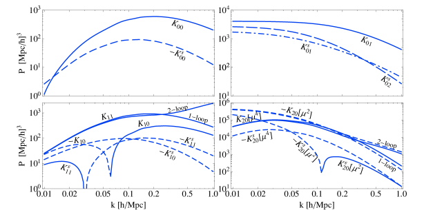
Figure 1: Kijsubscript𝐾𝑖𝑗K_{ij} terms using one loop PT results, and also two loop results for some of these terms. The terms proportional to bssubscript𝑏𝑠b_{s} are denoted with a subscript s𝑠s and can be compared to the term proportional to b2subscript𝑏2b_{2}. Solid lines are for positive values and dashed are for negative.

2.3.1 Nonlinear bias terms Kijsubscript𝐾𝑖𝑗K_{ij}

Modelling the biasing of dark matter halos beyond the linear bias b1subscript𝑏1b_{1} introduces additional 1-loop terms in perturbative approach. These terms are labeled here with Kijsubscript𝐾𝑖𝑗K_{ij} and will show up in the first few moment power spectra P00hh,P01hh,P02hhsubscriptsuperscript𝑃00subscriptsuperscript𝑃01subscriptsuperscript𝑃02P^{hh}_{00},P^{hh}_{01},P^{hh}_{02}, where b2subscript𝑏2b_{2}, bssubscript𝑏𝑠b_{s} and b3,nlsubscript𝑏3𝑛𝑙b_{3,nl} (the nonlocal third order bias [38, 40, 59]) appear at 1-loop level. In figure 1 we show the k-dependence of Kijsubscript𝐾𝑖𝑗K_{ij} terms. The relative contribution of these terms depends on the amplitudes of b2subscript𝑏2b_{2}, bssubscript𝑏𝑠b_{s} and b3,nlsubscript𝑏3𝑛𝑙b_{3,nl}. For example, one can use the values of b2subscript𝑏2b_{2}, bssubscript𝑏𝑠b_{s} from bispectrum [55, 40], where bssubscript𝑏𝑠b_{s} terms are small relative to the b2subscript𝑏2b_{2}. Taking into account also the k𝑘k-dependence of these terms we can see that effectively bssubscript𝑏𝑠b_{s} effects can be absorbed in the renormalized b2subscript𝑏2b_{2} value. For b3,nlsubscript𝑏3𝑛𝑙b_{3,nl} the corresponding trispectrum analysis has not been performed yet, but a power spectrum analysis together with the coevolution values [59] suggests that it can be important relative to b2subscript𝑏2b_{2}.

Over a limited range of interest where these terms matter and we are not too deeply into nonlinear regime, 0.05h/Mpc<k<0.2h/Mpc0.05𝑀𝑝𝑐𝑘0.2𝑀𝑝𝑐0.05h/Mpc<k<0.2h/Mpc, these terms can be organised (considering the k𝑘k-dependences and relative amplitudes) in a way that for each statistics we can define a single effective nonlinear bias parameter. In case of P00subscript𝑃00P_{00} we will denote it b200superscriptsubscript𝑏200b_{2}^{00}, and in case of P01subscript𝑃01P_{01}, b201superscriptsubscript𝑏201b_{2}^{01}.

2.3.2 Effective model for halo-halo power spectrum P00(hh)subscriptsuperscript𝑃00P^{(hh)}_{00}

Following the arguments from previous section we will absorb bssubscript𝑏𝑠b_{s} and b3,nlsubscript𝑏3𝑛𝑙b_{3,nl} terms into b2subscript𝑏2b_{2} and omit them from the analysis of P00hhsubscriptsuperscript𝑃00P^{hh}_{00} in this section. For a complete model of P00hhsubscriptsuperscript𝑃00P^{hh}_{00} from P00hmsubscriptsuperscript𝑃𝑚00P^{hm}_{00} we need to model the stochasticity term,

Λ(k)=P00,k(hh)2b1P00,k(hm)+b12P00,k(mm).Λ𝑘subscriptsuperscript𝑃00k2subscript𝑏1subscriptsuperscript𝑃𝑚00ksuperscriptsubscript𝑏12subscriptsuperscript𝑃𝑚𝑚00k\Lambda(k)=P^{(hh)}_{00,\textbf{k}}-2b_{1}P^{(hm)}_{00,\textbf{k}}+b_{1}^{2}P^{(mm)}_{00,\textbf{k}}. (2.22)

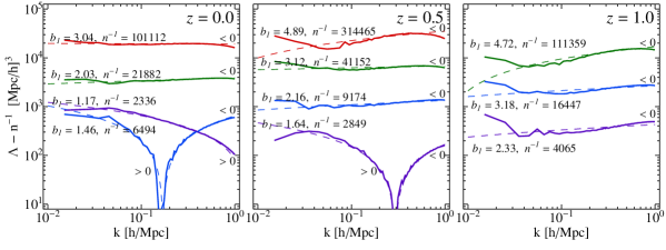
This term has recently been studied extensively in [58], where it is denoted as the diagonal term of the stochasticity matrix Cijsubscript𝐶𝑖𝑗C_{ij}. In the simplest models the stochasticity is given by the Poisson shot noise n¯1superscript¯𝑛1\bar{n}^{-1}, where n¯¯𝑛\bar{n} is the halo number density. As discussed in [58], there are deviations from this prediction sourced by both the halo exclusion and the nonlinear clustering of halos relative to dark matter: the latter can be seen from upper right panel of figure 1, where we see that all the terms are constant at low k𝑘k, suggesting a white noise contribution at low k𝑘k. Similarly, imposing a finite radius on halos lowers the stochasticity in the low k𝑘k limit below the Poisson n¯1superscript¯𝑛1\bar{n}^{-1} value. In the k0𝑘0k\rightarrow 0 limit one can determine from the clustering of halos in initial conditions: the dominant positive contribution comes from local biasing of initial halos and the negative contribution comes from exclusion. This limit does not change when evolving halos from initial to final redshift. The scale dependence of this term however changes from initial to final redshift and the theoretical modeling is still poorly understood. In this paper we add this model for the stochastic noise to our PT model of RSD and compare the result to the simulations. These shot noise effects are isotropic so the term does not have μ𝜇\mu dependence. It affects only the modelling of P00(hh)subscriptsuperscript𝑃00P^{(hh)}_{00} term, while all the higher order velocity moments contributions to RSD power spectra are independent of it. To determine it we use the N-body simulation measurements presented in [52, 54]. In figure 2 we show the results for Λ(k)Λ𝑘\Lambda(k) as measured from simulations, subtracting out the Poisson shot noise n¯1superscript¯𝑛1\bar{n}^{-1} (which are given in [54]). From the figure we see that deviations from Poisson model are of order 10-20% at low k𝑘k and thus cannot be neglected. Most of the plotted lines are negative, i.e. the measured stochasticity is sub-Poissonian, except for the lowest mass bins at redshift z=0.0𝑧0.0z=0.0 and z=0.5𝑧0.5z=0.5, where it is positive on large scales. As discussed in [60, 58] this is because exclusion dominates over nonlinear biasing for higher mass halos, while the opposite is true at low masses.
Refer to caption
Figure 2: The stochasticity as measured from the simulations, once the Poisson shot noise is subtracted (full lines). Four different mass bins are shown at the redshift z=0.0𝑧0.0z=0.0 and z=0.5𝑧0.5z=0.5 and three at the redshift z=1.0𝑧1.0z=1.0. Most of the plotted lines are negative, i.e. stochasticity is sub-Poissonian, except for the lowest mass bins at redshift z=0.0𝑧0.0z=0.0 and z=0.5𝑧0.5z=0.5 which are positive on large scales. Simple model from equation 2.23 is also shown (dashed lines).

To model this k𝑘k dependence on the scales of interest we propose a simple model

Λn¯1=λ+plogk,Λsuperscript¯𝑛1𝜆𝑝𝑘\Lambda-\bar{n}^{-1}=\lambda+p\log k, (2.23)

where we fit for the values of λ𝜆\lambda and p𝑝p and show the results in the same figure 2 as dashed lines. We see that this reproduces the measurements over a broad range of k𝑘k values, specially around k0.1h/Mpcsimilar-to𝑘0.1𝑀𝑝𝑐k\sim 0.1h/Mpc, where its effects are most important.

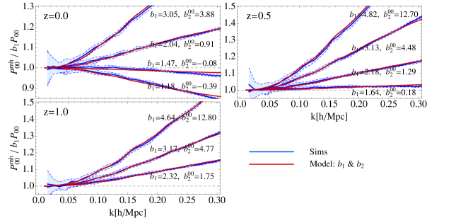
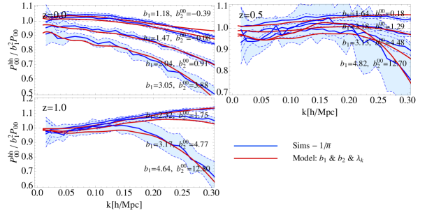
In figure 3 we show the scale dependence of the halo-matter cross power spectrum P00(hm)subscriptsuperscript𝑃𝑚00P^{(hm)}_{00} for several mass bins, at redshifts z=0.0𝑧0.0z=0.0, z=0.5𝑧0.5z=0.5 and z=1.0𝑧1.0z=1.0. We fit for an effective b200superscriptsubscript𝑏200b_{2}^{00} parameter to reproduce simulation measurements on the scales of interest and use these values then to model P00(hh)subscriptsuperscript𝑃00P^{(hh)}_{00}. In figure 4 we show the scale dependence of halo-halo auto power spectrum P00(hh)subscriptsuperscript𝑃00P^{(hh)}_{00} for the same mass bins as before, at reshifts z=0.0𝑧0.0z=0.0, z=0.5𝑧0.5z=0.5 and z=1.0𝑧1.0z=1.0. Using the stochasticity model presented above we evaluate it from

P00,k(hh)=2b1P00,k(hm)b12P00,k(mm)+Λ(k).subscriptsuperscript𝑃00k2subscript𝑏1subscriptsuperscript𝑃𝑚00ksuperscriptsubscript𝑏12subscriptsuperscript𝑃𝑚𝑚00kΛ𝑘P^{(hh)}_{00,\textbf{k}}=2b_{1}P^{(hm)}_{00,\textbf{k}}-b_{1}^{2}P^{(mm)}_{00,\textbf{k}}+\Lambda(k). (2.24)

In this model we also use simulation predictions for dark matter P00(mm)subscriptsuperscript𝑃𝑚𝑚00P^{(mm)}_{00} term at each of the redshifts.

Refer to caption
Figure 3: Scale dependence of halo-matter cross power spectrum P00(hm)subscriptsuperscript𝑃𝑚00P^{(hm)}_{00} is shown for several mass bins, at reshifts z=0.0𝑧0.0z=0.0, z=0.5𝑧0.5z=0.5 and z=1.0𝑧1.0z=1.0. Simulation measurements (blue solid line) are shown, as well as the results of the model presented in the text. We have fitted for b2subscript𝑏2b_{2} that reproduces best simulation measurements. All the lines are divided by b1subscript𝑏1b_{1} times the dark matter power spectrum from simulations.

2.4 P01(hh)subscriptsuperscript𝑃01P^{(hh)}_{01} term

Next we consider a correlation of the halo field and the halo momentum field. This term has only a scalar contribution and is the leading term in the μ2superscript𝜇2\mu^{2} dependence of the total redshift power spectrum, as was shown in [51, 53]. Here we generalize this terms to halos. Using definitions of the halo density 2.7 and momentum fields 2.9 we get

δh|T1h¯inner-productsuperscript𝛿superscriptsubscript𝑇1¯\displaystyle\left\langle\delta^{h}|T_{1}^{\bar{h}}\right\rangle =b1δ|(1+b¯1δ)u+12[b2δ2|u+bss2|u]+12b1b¯2δ|δ2vcabsentsubscript𝑏1inner-product𝛿1subscript¯𝑏1𝛿subscript𝑢parallel-to12delimited-[]subscript𝑏2inner-productsuperscript𝛿2subscript𝑢parallel-tosubscript𝑏𝑠inner-productsuperscript𝑠2subscript𝑢parallel-to12subscript𝑏1subscript¯𝑏2subscriptinner-product𝛿superscript𝛿2subscript𝑣parallel-to𝑐\displaystyle=b_{1}\left\langle\delta|(1+\bar{b}_{1}\delta)u_{\parallel}\right\rangle+\frac{1}{2}\Big{[}b_{2}\left\langle\delta^{2}|u_{\parallel}\right\rangle+b_{s}\left\langle s^{2}|u_{\parallel}\right\rangle\Big{]}+\frac{1}{2}b_{1}\bar{b}_{2}\left\langle\delta|\delta^{2}v_{\parallel}\right\rangle_{c}
+12b¯1[b2δ2|δu+bss2|δu]+14b2b2¯δ2|δ2vc+16b3δ3|uc,12subscript¯𝑏1delimited-[]subscript𝑏2inner-productsuperscript𝛿2𝛿subscript𝑢parallel-tosubscript𝑏𝑠inner-productsuperscript𝑠2𝛿subscript𝑢parallel-to14subscript𝑏2¯subscript𝑏2subscriptinner-productsuperscript𝛿2superscript𝛿2subscript𝑣parallel-to𝑐16subscript𝑏3subscriptinner-productsuperscript𝛿3subscript𝑢parallel-to𝑐\displaystyle+\frac{1}{2}\bar{b}_{1}\Big{[}b_{2}\left\langle\delta^{2}|\delta u_{\parallel}\right\rangle+b_{s}\left\langle s^{2}|\delta u_{\parallel}\right\rangle\Big{]}+\frac{1}{4}b_{2}\bar{b_{2}}\left\langle\delta^{2}|\delta^{2}v_{\parallel}\right\rangle_{c}+\frac{1}{6}b_{3}\left\langle\delta^{3}|u_{\parallel}\right\rangle_{c}, (2.25)

where we have used the same renormalization scheme as for P00(hh)subscriptsuperscript𝑃00P^{(hh)}_{00} term. Subscript c𝑐c stands for the connected part of the correlator, while the disconnected parts get renormalized. Keeping the terms at one loop order we get for the power spectrum,

P01,k(hh¯)=b1b¯1P01,k+b1(1b¯1)αPδθ,k+α[b2K10,k+bsK10,ks]+αb¯1[b2K11,k+bsK11,ks],subscriptsuperscript𝑃¯01ksubscript𝑏1subscript¯𝑏1subscript𝑃01ksubscript𝑏11subscript¯𝑏1𝛼subscript𝑃𝛿𝜃k𝛼delimited-[]subscript𝑏2subscript𝐾10ksubscript𝑏𝑠subscriptsuperscript𝐾𝑠10k𝛼subscript¯𝑏1delimited-[]subscript𝑏2subscript𝐾11ksubscript𝑏𝑠subscriptsuperscript𝐾𝑠11k\displaystyle P^{(h\bar{h})}_{01,\textbf{k}}=b_{1}\bar{b}_{1}P_{01,\textbf{k}}+b_{1}(1-\bar{b}_{1})\alpha P_{\delta\theta,\textbf{k}}+\alpha\Big{[}b_{2}K_{10,\textbf{k}}+b_{s}K^{s}_{10,\textbf{k}}\Big{]}+\alpha\bar{b}_{1}\Big{[}b_{2}K_{11,\textbf{k}}+b_{s}K^{s}_{11,\textbf{k}}\Big{]}, (2.26)

where we have α=iμ/k𝛼𝑖𝜇𝑘\alpha=-i\mu/k. Using the PT to evaluate the contributions of nonlinear biasing terms we get

K10,ksubscript𝐾10k\displaystyle K_{10,\textbf{k}} Pq(L)Pkq(L)Gq,kq(2),absentsubscriptsuperscript𝑃𝐿qsubscriptsuperscript𝑃𝐿kqsubscriptsuperscript𝐺2qkq\displaystyle\equiv P^{(L)}_{\textbf{q}}P^{(L)}_{\textbf{k}-\textbf{q}}G^{(2)}_{\textbf{q},\textbf{k}-\textbf{q}},
K10,kssubscriptsuperscript𝐾𝑠10k\displaystyle K^{s}_{10,\textbf{k}} Pq(L)Pkq(L)Gq,kq(2)Sq,kq(2),absentsubscriptsuperscript𝑃𝐿qsubscriptsuperscript𝑃𝐿kqsubscriptsuperscript𝐺2qkqsubscriptsuperscript𝑆2qkq\displaystyle\equiv P^{(L)}_{\textbf{q}}P^{(L)}_{\textbf{k}-\textbf{q}}G^{(2)}_{\textbf{q},\textbf{k}-\textbf{q}}S^{(2)}_{\textbf{q},\textbf{k}-\textbf{q}},
K11,ksubscript𝐾11k\displaystyle K_{11,\textbf{k}} kxqPq(L)Pkq(L),absent𝑘𝑥𝑞subscriptsuperscript𝑃𝐿qsubscriptsuperscript𝑃𝐿kq\displaystyle\equiv\frac{kx}{q}P^{(L)}_{\textbf{q}}P^{(L)}_{\textbf{k}-\textbf{q}},
K11,kssubscriptsuperscript𝐾𝑠11k\displaystyle K^{s}_{11,\textbf{k}} kxqPq(L)Pkq(L)Sq,kq(2),absent𝑘𝑥𝑞subscriptsuperscript𝑃𝐿qsubscriptsuperscript𝑃𝐿kqsubscriptsuperscript𝑆2qkq\displaystyle\equiv\frac{kx}{q}P^{(L)}_{\textbf{q}}P^{(L)}_{\textbf{k}-\textbf{q}}S^{(2)}_{\textbf{q},\textbf{k}-\textbf{q}}, (2.27)

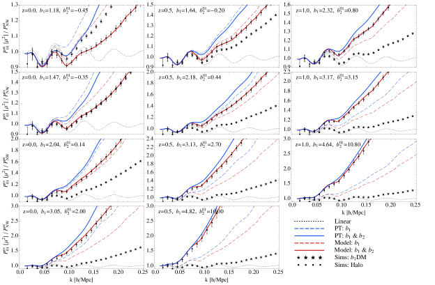
where again the integration over q𝑞q variable is implied and G(2)superscript𝐺2G^{(2)} is the standard kernel of velocity divergence in Eulerian PT (e.g. [22, 53]). In figure 5 we show the results for halo-halo P01subscript𝑃01P_{01} modelling, and comparison to the N-body simulation results. The model presented in 2.26 contains dark matter parts, P01subscript𝑃01P_{01} and Pδθsubscript𝑃𝛿𝜃P_{\delta\theta} that were already extensively discussed in [53]. These two contributions we actually measure from the simulations in order to focus on the bias modelling and reduce potential degeneracy with PT modelling. It is also good to note that on the scales of interest, using Pδθsubscript𝑃𝛿𝜃P_{\delta\theta} either measured from simulations or predicted by PT has only a slight impact on best fit value of b201subscriptsuperscript𝑏012b^{01}_{2}. We use the b1subscript𝑏1b_{1} values determined from the matter-halo power spectra P00(hm)subscriptsuperscript𝑃𝑚00P^{(hm)}_{00} from previous section. Note that the relative contributions from b2subscript𝑏2b_{2} and b3,nlsubscript𝑏3𝑛𝑙b_{3,nl} terms in P01,k(hh¯)subscriptsuperscript𝑃¯01kP^{(h\bar{h})}_{01,\textbf{k}} differ from those in P00,k(hh¯)subscriptsuperscript𝑃¯00kP^{(h\bar{h})}_{00,\textbf{k}}, but the scale dependence of these terms is similar over the limited range of scale of interest here (0.05h/Mpc<k<0.2h/Mpc0.05𝑀𝑝𝑐𝑘0.2𝑀𝑝𝑐0.05h/Mpc<k<0.2h/Mpc). This again suggests we can replace all the nonlinear bias terms with a single effective b201superscriptsubscript𝑏201b_{2}^{01}, which however can take a different numerical value from b200superscriptsubscript𝑏200b_{2}^{00}. We thus fit for a new set of b201superscriptsubscript𝑏201b_{2}^{01} values in order to achieve better correspondence with the halo simulation results. In the same figure we also show the results using just the linear biasing b1subscript𝑏1b_{1}.

Refer to caption
Figure 4: Scale dependence of halo-halo auto power spectrum P00(hh)subscriptsuperscript𝑃00P^{(hh)}_{00} shown for several mass bins, at reshifts z=0.0𝑧0.0z=0.0, z=0.5𝑧0.5z=0.5 and z=1.0𝑧1.0z=1.0. Simulation measurements (blue solid line) are shown, as well as the results of the model presented in the text. All the lines are divided by the b12superscriptsubscript𝑏12b_{1}^{2} times the dark matter power spectrum from the simulations.
Refer to caption
Figure 5: Halo-halo density-momentum power spectrum P01subscript𝑃01P_{01} for four mass bins, at reshifts z=0.0𝑧0.0z=0.0, z=0.5𝑧0.5z=0.5 and z=1.0𝑧1.0z=1.0. We show SPT results (blue lines) and, because SPT does not reproduce DM simulations well, we also show results using the model where we use DM simulations for linear biasing terms (red lines) to isolate the biasing effects in RSD. For comparison we also show linear biasing (dashed lines) and nonlinear biasing (solid lines) models. Halo (black points) simulation data and b1subscript𝑏1b_{1} times the dark matter data (black stars) are also shown. All the spectra are divided by the no wiggle linear prediction [61] for b1P01subscript𝑏1subscript𝑃01b_{1}P_{01} term.

2.4.1 On the different b2subscript𝑏2b_{2} values for P00(hm)superscriptsubscript𝑃00𝑚P_{00}^{(hm)} and P01(hh)superscriptsubscript𝑃01P_{01}^{(hh)}

As was mentioned above two different sets of b2subscript𝑏2b_{2} parameters are used: one set to model matter halo-cross power spectrum P00(hm)subscriptsuperscript𝑃𝑚00P^{(hm)}_{00} and, consequently, halo-halo auto power spectra P00(hh)subscriptsuperscript𝑃00P^{(hh)}_{00}, and the second set to model the predictions for P01(hh)subscriptsuperscript𝑃01P^{(hh)}_{01}. We have argued that this is necessary because there are several free bias parameters that enter the power spectra at 1-loop level, all of which have a similar scale dependence, which means we cannot determine them individually and we have replaced them with a single effective b2subscript𝑏2b_{2} parameter instead. However, while for each statistic we can replace them all with a single effective parameter, the relative contributions from each physical nonlinear bias to different statistics changes, so the values of the effective parameters can change as well.

One wishes to have a biasing model valid for all the statistics of interest and thus for all the correlators used in our RSD model. Ideally this would also include the higher order correlations, as well as all correlations with the dark matter. It is important to realize that this difference in b2subscript𝑏2b_{2} bias stays at the level of P00subscript𝑃00P_{00} and P01subscript𝑃01P_{01} correlators, since all the higher order correlators come only through these two terms, at least at one loop level we work here. So one can ask whether one can explain the difference using a physically motivated model of nonlinear biasing. We find that bssubscript𝑏𝑠b_{s} does not seem to matter much assuming its values from the bispectrum analysis [55, 39], or its values from the coevolution model assuming it is zero in initial conditions, and so can be ignored. In contrast, b2subscript𝑏2b_{2} and b3,nlsubscript𝑏3𝑛𝑙b_{3,nl} appear to be equally important [38, 59]. For the terms we are discussing, this gives

P00,k(hh)=subscriptsuperscript𝑃00kabsent\displaystyle P^{(hh)}_{00,\textbf{k}}= b12P00,k+2b1[b2K00,k+bsK00,ks]+12[b22K01,k+bs2K01,ks]superscriptsubscript𝑏12subscript𝑃00k2subscript𝑏1delimited-[]subscript𝑏2subscript𝐾00ksubscript𝑏𝑠subscriptsuperscript𝐾𝑠00k12delimited-[]subscriptsuperscript𝑏22subscript𝐾01ksubscriptsuperscript𝑏2𝑠subscriptsuperscript𝐾𝑠01k\displaystyle b_{1}^{2}P_{00,\textbf{k}}+2b_{1}\Big{[}b_{2}K_{00,\textbf{k}}+b_{s}K^{s}_{00,\textbf{k}}\Big{]}+\frac{1}{2}\Big{[}b^{2}_{2}K_{01,\textbf{k}}+b^{2}_{s}K^{s}_{01,\textbf{k}}\Big{]}
+b2bsK02,ks+2b3,nlσ3,k2Pk(L),subscript𝑏2subscript𝑏𝑠subscriptsuperscript𝐾𝑠02k2subscript𝑏3𝑛𝑙superscriptsubscript𝜎3𝑘2subscriptsuperscript𝑃𝐿𝑘\displaystyle+b_{2}b_{s}K^{s}_{02,\textbf{k}}+2b_{3,nl}\sigma_{3,k}^{2}P^{(L)}_{k}, (2.28)

and also

P01,k(hh)=subscriptsuperscript𝑃01kabsent\displaystyle P^{(hh)}_{01,\textbf{k}}= b12P01,k+b1(1b1)αPδθ,k+α[b2K10,k+bsK10,ks]superscriptsubscript𝑏12subscript𝑃01ksubscript𝑏11subscript𝑏1𝛼subscript𝑃𝛿𝜃k𝛼delimited-[]subscript𝑏2subscript𝐾10ksubscript𝑏𝑠subscriptsuperscript𝐾𝑠10k\displaystyle b_{1}^{2}P_{01,\textbf{k}}+b_{1}(1-b_{1})\alpha P_{\delta\theta,\textbf{k}}+\alpha\Big{[}b_{2}K_{10,\textbf{k}}+b_{s}K^{s}_{10,\textbf{k}}\Big{]}
+αb1[b2K11,k+bsK11,ks]+αb3,nlσ3,k2Pk(L),𝛼subscript𝑏1delimited-[]subscript𝑏2subscript𝐾11ksubscript𝑏𝑠subscriptsuperscript𝐾𝑠11k𝛼subscript𝑏3𝑛𝑙superscriptsubscript𝜎3𝑘2subscriptsuperscript𝑃𝐿𝑘\displaystyle+\alpha b_{1}\Big{[}b_{2}K_{11,\textbf{k}}+b_{s}K^{s}_{11,\textbf{k}}\Big{]}+\alpha b_{3,nl}\sigma_{3,k}^{2}P^{(L)}_{k}, (2.29)

where σ3,ksubscript𝜎3𝑘\sigma_{3,k} is defined in [38] and for detailed discussion of these terms we refer to [59]. The coevolution model predicts a specific value for b3,nlsubscript𝑏3𝑛𝑙b_{3,nl} today assuming it is zero initially [39]. Using these predicted values we can predict the difference between the two effective b2subscript𝑏2b_{2} values: we find that this model indeed predicts that b200superscriptsubscript𝑏200b_{2}^{00} is larger than b201superscriptsubscript𝑏201b_{2}^{01} and that the amplitude of the difference increases with halo bias b1subscript𝑏1b_{1}. The prediction of this model is shown in figure 6, together with the results from the fits. We show the redshift dependence of b2subscript𝑏2b_{2} on b1subscript𝑏1b_{1} and the difference Δb2=b200b201Δsubscript𝑏2subscriptsuperscript𝑏002subscriptsuperscript𝑏012\Delta b_{2}=b^{00}_{2}-b^{01}_{2}.

Even having these three nonlocal bias models may not be all that is required for a complete model: in the peak model one expects to have k2superscript𝑘2k^{2} corrections to linear bias both in the halo density and in the halo velocity in the initial conditions [62, 57]. If shown to be significant at later times of evolution, this could play an important role in modelling of all velocity correlators.

2.5 P02(hh)subscriptsuperscript𝑃02P^{(hh)}_{02} term

Refer to caption
Figure 6: Comparison of b200superscriptsubscript𝑏200b_{2}^{00} and b201superscriptsubscript𝑏201b_{2}^{01} used in modelling of P00subscript𝑃00P_{00} and P01subscript𝑃01P_{01} terms. In the left panel we show redshift dependence of b2/b1subscript𝑏2subscript𝑏1b_{2}/b_{1} values for P00subscript𝑃00P_{00} term (blue) and P01subscript𝑃01P_{01} (red) term. In the right panel we show the dependence of the difference Δb2=b200b201Δsubscript𝑏2subscriptsuperscript𝑏002subscriptsuperscript𝑏012\Delta b_{2}=b^{00}_{2}-b^{01}_{2} on the values of b1subscript𝑏1b_{1}. We show results for redshift z=0.0𝑧0.0z=0.0 (blue), z=0.5𝑧0.5z=0.5 (red) and z=1.0𝑧1.0z=1.0 (green).

Next term we are considering is the correlation of the halo field with the halo kinetic energy density field. This term has the only scalar part but these give the contributions to both μ2superscript𝜇2\mu^{2} and μ4superscript𝜇4\mu^{4} parts of the total redshift power spectrum. We have

δh|T2h¯inner-productsuperscript𝛿superscriptsubscript𝑇2¯\displaystyle\left\langle\delta^{h}|T_{2}^{\bar{h}}\right\rangle =b1δ|u2+b1b¯1δ|δu2+12b2δ2|u2+12bss2|u2absentsubscript𝑏1inner-product𝛿subscriptsuperscript𝑢2parallel-tosubscript𝑏1subscript¯𝑏1inner-product𝛿𝛿subscriptsuperscript𝑢2parallel-to12subscript𝑏2inner-productsuperscript𝛿2superscriptsubscript𝑢parallel-to212subscript𝑏𝑠inner-productsuperscript𝑠2superscriptsubscript𝑢parallel-to2\displaystyle=b_{1}\left\langle\delta|u^{2}_{\parallel}\right\rangle+b_{1}\bar{b}_{1}\left\langle\delta|\delta u^{2}_{\parallel}\right\rangle+\frac{1}{2}b_{2}\left\langle\delta^{2}|u_{\parallel}^{2}\right\rangle+\frac{1}{2}b_{s}\left\langle s^{2}|u_{\parallel}^{2}\right\rangle
+12b¯1b2δ2|δu2+12b1b¯2δ|δ2u2c+14b2b¯2δ2|δ2u2c12subscript¯𝑏1subscript𝑏2inner-productsuperscript𝛿2𝛿superscriptsubscript𝑢parallel-to212subscript𝑏1subscript¯𝑏2subscriptinner-product𝛿superscript𝛿2superscriptsubscript𝑢parallel-to2𝑐14subscript𝑏2subscript¯𝑏2subscriptinner-productsuperscript𝛿2superscript𝛿2superscriptsubscript𝑢parallel-to2𝑐\displaystyle+\frac{1}{2}\bar{b}_{1}b_{2}\left\langle\delta^{2}|\delta u_{\parallel}^{2}\right\rangle+\frac{1}{2}b_{1}\bar{b}_{2}\left\langle\delta|\delta^{2}u_{\parallel}^{2}\right\rangle_{c}+\frac{1}{4}b_{2}\bar{b}_{2}\left\langle\delta^{2}|\delta^{2}u_{\parallel}^{2}\right\rangle_{c} (2.30)

where we have used the same renormalization scheme as for P00(hh)subscriptsuperscript𝑃00P^{(hh)}_{00} term. Subscript c𝑐c stands for the connected part of the correlator, while the disconnected parts of this terms get renormalized. We get for the power spectrum of this term

P02,k(hh¯)=b1P¯02,k+P00,khhσv2[b2K20,k+bsK20,ks],subscriptsuperscript𝑃¯02ksubscript𝑏1subscript¯𝑃02ksubscriptsuperscript𝑃00ksuperscriptsubscript𝜎𝑣2delimited-[]subscript𝑏2subscript𝐾20ksubscript𝑏𝑠subscriptsuperscript𝐾𝑠20k\displaystyle P^{(h\bar{h})}_{02,\textbf{k}}=b_{1}\bar{P}_{02,\textbf{k}}+P^{hh}_{00,\textbf{k}}\sigma_{v}^{2}-\Big{[}b_{2}K_{20,\textbf{k}}+b_{s}K^{s}_{20,\textbf{k}}\Big{]}, (2.31)

where the first term is the reduced dark matter contribution δ|vcproportional-toabsentsubscriptinner-product𝛿subscript𝑣parallel-to𝑐\propto\left\langle\delta|v_{\parallel}\right\rangle_{c} as defined in [53]. Nonlinear bias comes in through the biasing in P00hhsubscriptsuperscript𝑃00P^{hh}_{00} term and we also have the contributions of two additional terms

K20,ksubscript𝐾20k\displaystyle K_{20,\textbf{k}} qq2(kq)(kq)2Pq(L)Pkq(L),absentsubscript𝑞parallel-tosuperscript𝑞2subscriptkqparallel-tosuperscriptkq2subscriptsuperscript𝑃𝐿qsubscriptsuperscript𝑃𝐿kq\displaystyle\equiv\frac{q_{\parallel}}{q^{2}}\frac{(\textbf{k}-\textbf{q})_{\parallel}}{(\textbf{k}-\textbf{q})^{2}}P^{(L)}_{\textbf{q}}P^{(L)}_{\textbf{k}-\textbf{q}},
K20,kssubscriptsuperscript𝐾𝑠20k\displaystyle K^{s}_{20,\textbf{k}} qq2(kq)(kq)2Pq(L)Pkq(L)Sq,kq(2).absentsubscript𝑞parallel-tosuperscript𝑞2subscriptkqparallel-tosuperscriptkq2subscriptsuperscript𝑃𝐿qsubscriptsuperscript𝑃𝐿kqsubscriptsuperscript𝑆2qkq\displaystyle\equiv\frac{q_{\parallel}}{q^{2}}\frac{(\textbf{k}-\textbf{q})_{\parallel}}{(\textbf{k}-\textbf{q})^{2}}P^{(L)}_{\textbf{q}}P^{(L)}_{\textbf{k}-\textbf{q}}S^{(2)}_{\textbf{q},\textbf{k}-\textbf{q}}. (2.32)

These terms have contributions to both μ2superscript𝜇2\mu^{2} and μ4superscript𝜇4\mu^{4}. As was shown in [53], the term that is proportional to the velocity dispersion will appear in the μ2superscript𝜇2\mu^{2} part. Since for DM it is not possible to evaluate the total velocity dispersion using PT we had to model small scale contributions adding a part which was motivated by the velocity dispersion in a halo using the halo model. For halos the situation is simpler in that we do not expect such a term to be present, as there is no small scale velocity dispersion contribution, and hence no FoG. Most of the contribution comes from the large scale velocities which can at least in principle be described using PT.

2.5.1 Velocity dispersion predictions and simulation measurements
Refer to caption
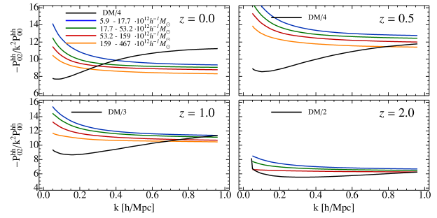
Figure 7: P02/P00subscript𝑃02subscript𝑃00P_{02}/P_{00} for halos and dark matter. Results are presented for dark matter halos (color coding for respective bias values) and for the dark matter (in black). Values of velocity dispersion can be estimated at the smaller scale regions (higher k𝑘k), where the ratio tends approach the constant values. We show the ratio for four different halo mass bins and for four different redshifts.
Refer to caption
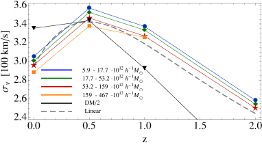
Figure 8: Redshift dependence of the halo velocity dispersion measurements obtained from simulations. Four different mass bins values are shown (in different color coding respectively). We also show the velocity dispersion measurements for dark matter case (in Black). Also shown are the linear theory prediction for velocity dispersion values (gray dashed line). Notice that the values of measured velocity dispersion have a weak dependence on mass of the halo bins.

In order to test the velocity dispersion behaviour in more detail let us consider more closely the contribution of μ2superscript𝜇2\mu^{2} part of P02hhsubscriptsuperscript𝑃02P^{hh}_{02}. From previous work on dark matter [53], we have seen that on quasi-nonlinear scales most of the contributions to the P02subscript𝑃02P_{02} term came from the part proportional to the factor corresponding to the dark matter velocity dispersion multiplied with P00subscript𝑃00P_{00} term. For halos this will be generalized to the σv2P00hhsubscriptsuperscript𝜎2𝑣subscriptsuperscript𝑃00\sigma^{2}_{v}P^{hh}_{00}, where we have the halo velocity dispersion instead. In order to test the behaviour on the halo velocity dispersion in simulations, in figure 7 we show the k𝑘k dependence of P02hh/P00hhsubscriptsuperscript𝑃02subscriptsuperscript𝑃00P^{hh}_{02}/P^{hh}_{00}. From the figure it can be seen that at smaller scales this ratio tends to a constant for all mass bins and redshifts. This constant values can be interpreted as the halo velocity dispersion σv2subscriptsuperscript𝜎2𝑣\sigma^{2}_{v}. Note that for this figure we include the shot noise n¯1superscript¯𝑛1\bar{n}^{-1} in P00hhsubscriptsuperscript𝑃00P^{hh}_{00}, and we expect there is also the shot noise σv2/n¯superscriptsubscript𝜎𝑣2¯𝑛\sigma_{v}^{2}/\bar{n} in P02subscript𝑃02P_{02}.

In figure 8 we show the redshift dependence of the halo velocity dispersion σvsubscript𝜎𝑣\sigma_{v} as obtained from simulations (high-k regime in figure 7). We see the trend of the velocity dispersion values increasing and then decreasing with redshift, as predicted by the linear theory prediction of the velocity dispersion

σv,lin2(τ)=13d3q(2π)3Pθθ(q,τ)q2.superscriptsubscript𝜎𝑣lin2𝜏13superscript𝑑3𝑞superscript2𝜋3subscript𝑃𝜃𝜃𝑞𝜏superscript𝑞2\sigma_{v,\text{lin}}^{2}(\tau)=\frac{1}{3}\int{\frac{d^{3}q}{(2\pi)^{3}}\frac{P_{\theta\theta}(q,\tau)}{q^{2}}}. (2.33)

We see that velocity dispersions weakly depend on the masses of the halos, at all the redshifts, and are in a good agreement with linear theory predictions. In contrast, the dark matter velocity dispersion is significantly higher than the linear theory prediction. Slight dependence of halo velocity dispersion on halo mass, noticeable in figures 7 and 8 can be explained by the terms in equation 2.31 that do not depend on σvsubscript𝜎𝑣\sigma_{v}. Higher order terms can also play a role in modelling both δh|u2inner-productsuperscript𝛿superscriptsubscript𝑢parallel-to2\left\langle\delta^{h}|u_{\parallel}^{2}\right\rangle and also connected term δh|δhu2inner-productsuperscript𝛿superscript𝛿superscriptsubscript𝑢parallel-to2\left\langle\delta^{h}|\delta^{h}u_{\parallel}^{2}\right\rangle.

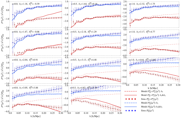
In figure 9 we show the μ2superscript𝜇2\mu^{2} part of P02(hh)+P11(hh)subscriptsuperscript𝑃02subscriptsuperscript𝑃11P^{(hh)}_{02}+P^{(hh)}_{11} and μ4superscript𝜇4\mu^{4} part of P02(hh)subscriptsuperscript𝑃02P^{(hh)}_{02} as contributions to the total redshift power spectrum. The sum of P02(hh)subscriptsuperscript𝑃02P^{(hh)}_{02} and P11(hh)subscriptsuperscript𝑃11P^{(hh)}_{11} terms is chosen since both of these terms have isotropic shot noise contributions σ2/n¯superscript𝜎2¯𝑛\sigma^{2}/\bar{n}, and which can be large for rare tracers such as halos. Since these two contributions come with opposite signs and exactly cancel in the sum, they give no residual shot noise contribution to the total RSD power spectrum . From equation 2.31 we see that P02hhsubscriptsuperscript𝑃02P^{{hh}}_{02} term also contains contributions from P00hhsubscriptsuperscript𝑃00P^{{hh}}_{00} term which contains nonlinear b2subscript𝑏2b_{2} bias. Thus for modelling the P02hhsubscriptsuperscript𝑃02P^{{hh}}_{02} term we use the same b2subscript𝑏2b_{2} values as for P00hhsubscriptsuperscript𝑃00P^{{hh}}_{00} term.

Refer to caption
Figure 9: μ2superscript𝜇2\mu^{2} part of P02+P11subscript𝑃02subscript𝑃11P_{02}+P_{11} (red color) and μ4superscript𝜇4\mu^{4} part of P02subscript𝑃02P_{02} (blue color) is shown at three different redsifts, for several mass bins. Simulation measurements (points) of these two terms are compared to the model 2.31 using linear (dashed lines) and non-linear (solid lines) biasing. All the plots are divided by the linear predictions k2σv2PNWsuperscript𝑘2superscriptsubscript𝜎𝑣2subscript𝑃𝑁𝑊k^{2}\sigma_{v}^{2}P_{NW} with no BAO wiggles.

2.6 P11(hh)subscriptsuperscript𝑃11P^{(hh)}_{11} term

Next term to consider is the autocorrelation of the halo momentum field P11(hh)subscriptsuperscript𝑃11P^{(hh)}_{11}. This term will give the contributions to both μ2superscript𝜇2\mu^{2} (which has only contributions from the vector part) and μ4superscript𝜇4\mu^{4} angular dependence (which has dominantly contributions from the scalar part on large scales, as it is present already in linear theory, while the vector part becomes important on small scales). Leading term on the large scales has μ4superscript𝜇4\mu^{4} angular dependence and in the limit of small k𝑘k consists only of the third Kaiser term. Correlating the two halo momentum fields using the biasing model (equation 2.9) we get

T1h|T1h¯inner-productsuperscriptsubscript𝑇1superscriptsubscript𝑇1¯\displaystyle\left\langle T_{1}^{h}|T_{1}^{\bar{h}}\right\rangle =u|u+(b1+b¯1)u|δu+b1b¯1δu|δuabsentinner-productsubscript𝑢parallel-tosubscript𝑢parallel-tosubscript𝑏1subscript¯𝑏1inner-productsubscript𝑢parallel-to𝛿subscript𝑢parallel-tosubscript𝑏1subscript¯𝑏1inner-product𝛿subscript𝑢parallel-to𝛿subscript𝑢parallel-to\displaystyle=\left\langle u_{\parallel}|u_{\parallel}\right\rangle+(b_{1}+\bar{b}_{1})\left\langle u_{\parallel}|\delta u_{\parallel}\right\rangle+b_{1}\bar{b}_{1}\left\langle\delta u_{\parallel}|\delta u_{\parallel}\right\rangle
+12(b2+b¯2)u|δ2uc+{b1,b2}δu|δ2uc+14b2b¯2δ2u|δ2uc12subscript𝑏2subscript¯𝑏2subscriptinner-productsubscript𝑢parallel-tosuperscript𝛿2subscript𝑢parallel-to𝑐subscript𝑏1subscript𝑏2subscriptinner-product𝛿subscript𝑢parallel-tosuperscript𝛿2subscript𝑢parallel-to𝑐14subscript𝑏2subscript¯𝑏2subscriptinner-productsuperscript𝛿2subscript𝑢parallel-tosuperscript𝛿2subscript𝑢parallel-to𝑐\displaystyle+\frac{1}{2}(b_{2}+\bar{b}_{2})\left\langle u_{\parallel}|\delta^{2}u_{\parallel}\right\rangle_{c}+\left\{b_{1},b_{2}\right\}\left\langle\delta u_{\parallel}|\delta^{2}u_{\parallel}\right\rangle_{c}+\frac{1}{4}b_{2}\bar{b}_{2}\left\langle\delta^{2}u_{\parallel}|\delta^{2}u_{\parallel}\right\rangle_{c} (2.34)

where we can again use the same renormalization scheme as for P00(hh)subscriptsuperscript𝑃00P^{(hh)}_{00} term. Subscript c𝑐c again represents connected part of the correlator, while the disconnected parts gets renormalized. Keeping the terms at one loop order we get for the power spectrum,

P11,k(h1h2)=P11,k+[(b11)+(b¯11)]μkB11,k+(b1b¯11)C11,k,subscriptsuperscript𝑃subscript1subscript211ksubscript𝑃11kdelimited-[]subscript𝑏11subscript¯𝑏11𝜇𝑘subscript𝐵11ksubscript𝑏1subscript¯𝑏11subscript𝐶11k\displaystyle P^{(h_{1}h_{2})}_{11,\textbf{k}}=P_{11,\textbf{k}}+\big{[}(b_{1}-1)+(\bar{b}_{1}-1)\big{]}\frac{\mu}{k}B_{11,\textbf{k}}+(b_{1}\bar{b}_{1}-1)C_{11,\textbf{k}}, (2.35)

where the dark matter terms P11subscript𝑃11P_{11}, B11subscript𝐵11B_{11} and C11subscript𝐶11C_{11} used here have been computed in [53]. At the one loop level of PT modelling, there are no contributions of b2subscript𝑏2b_{2} bias terms, as can be seen from 2.34 where all b2subscript𝑏2b_{2} terms appear only at the 2-loop level. The same is true for higher order local and nonlocal bias contributions.

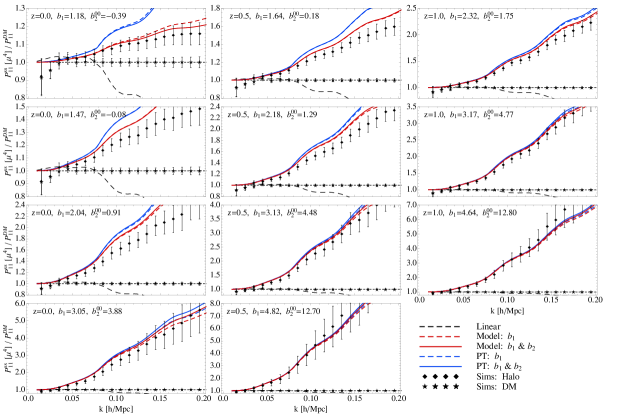
In figure 10 we show the scalar part of velocity moment halo power spectra P11(hh)subscriptsuperscript𝑃11P^{(hh)}_{11}. To improve the precision we use simulations for the scalar part of P11subscript𝑃11P_{11} for dark matter. For a more extensive discussion about how to model this in PT and consistency of this procedure we refer to [53]. We also investigate the two loop contributions and show terms proportional to b2subscript𝑏2b_{2} in equation 2.34. Notice that these contributions are suppressed by the f2D6superscript𝑓2superscript𝐷6f^{2}D^{6} factor so the contribution at higher redshifts quickly becomes less important. Overall we see that the model qualitatively reproduces simulations well, but not quantitatively for all halos. Notice the very strong scale dependence of the term, specially for the highly biased halos. The scale dependence is induced already at the linear biasing level. As mentioned in previous section, vector part of P11(hh)subscriptsuperscript𝑃11P^{(hh)}_{11} is shown in figure 9 where it is combined with μ2superscript𝜇2\mu^{2} part of the P02(hh)subscriptsuperscript𝑃02P^{(hh)}_{02} term. Overall we conclude that our model reproduces all the trends seen in simulations without any additional free parameters (except the b1subscript𝑏1b_{1} and b2subscript𝑏2b_{2} bias parameters that have been fitted to measurement of P00(hh)superscriptsubscript𝑃00P_{00}^{(hh)} and P01(hh)superscriptsubscript𝑃01P_{01}^{(hh)}), but is not sufficient to achieve high precision predictions down to very small scales.
Refer to caption
Figure 10: μ4superscript𝜇4\mu^{4} part of the halo momentum power spectrum P11(hh)subscriptsuperscript𝑃11P^{(hh)}_{11} relative to P11subscript𝑃11P_{11} for dark matter. Results are shown for halos for several mass bins at redshifts z=0.0,0.5,1.0𝑧0.00.51.0z=0.0,~{}0.5,~{}1.0. We show the full SPT result (blue line) and the model (red line) where simulations are used for the DM part of P11subscript𝑃11P_{11}. Both the linear biasing model (dashed lines) and the nonlinear biasing model with b2subscript𝑏2b_{2} terms is shown (solid line). Here we emphasize that the b2subscript𝑏2b_{2} parameters are not free, but have been fixed by the P00subscript𝑃00P_{00} and P01subscript𝑃01P_{01} analyses. We also show the halo simulation measurements (black dots) and b1subscript𝑏1b_{1} times DM simulations (black stars). Kaiser linear result with b1subscript𝑏1b_{1} bias is also shown (lond-dashed black line).

2.7 P12(hh)subscriptsuperscript𝑃12P^{(hh)}_{12} and P03(hh)subscriptsuperscript𝑃03P^{(hh)}_{03} terms

Refer to caption
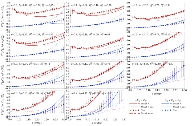
Figure 11: μ4superscript𝜇4\mu^{4} parts of the P12+P03subscript𝑃12subscript𝑃03P_{12}+P_{03} (red) term and P13+P22+P04subscript𝑃13subscript𝑃22subscript𝑃04P_{13}+P_{22}+P_{04} (blue) for several mass bins at redshifts z=0.0,0.5,1.0𝑧0.00.51.0z=0.0,~{}0.5,~{}1.0. We take the specific combinations for which the shot noise contributions cancel out. We show results for the linear biasing model (dashed) and for the nonlinear biasing (solid). Note the large effect of nonlinear biasing. Here again we emphasize that the b2subscript𝑏2b_{2} parameters are not free, but have been fixed by the P00subscript𝑃00P_{00} and P01subscript𝑃01P_{01} analyses. For P12+P03subscript𝑃12subscript𝑃03P_{12}+P_{03} term we also present a hybrid result (red dot-dashed line) where we fit for the correction in the lowest mass bin at each redshift and apply it to higher mass bins. All the plots are divided by the linear predictions b1k2σv2PNWsubscript𝑏1superscript𝑘2superscriptsubscript𝜎𝑣2subscript𝑃𝑁𝑊b_{1}k^{2}\sigma_{v}^{2}P_{NW} with no BAO wiggles.

In this subsection we look at higher order moment terms P12(hh)subscriptsuperscript𝑃12P^{(hh)}_{12} and P03(hh)subscriptsuperscript𝑃03P^{(hh)}_{03} which have the lowest angular contribution at μ4superscript𝜇4\mu^{4} level. We will only model the lowest order μ4superscript𝜇4\mu^{4} terms, which give the nonlinear corrections to the last Kaiser term. Nonlinear b2subscript𝑏2b_{2} bias enter in these terms indirectly through the terms P00(hh)subscriptsuperscript𝑃00P^{(hh)}_{00}, P01(hh)subscriptsuperscript𝑃01P^{(hh)}_{01} and consequently P11(hh)subscriptsuperscript𝑃11P^{(hh)}_{11}. For the correlation of first and second order momentum fields P12(hh¯)subscriptsuperscript𝑃¯12P^{(h\bar{h})}_{12} we have

T1h|T2h¯inner-productsuperscriptsubscript𝑇1superscriptsubscript𝑇2¯\displaystyle\left\langle T_{1}^{h}|T_{2}^{\bar{h}}\right\rangle =(1+δh)u|(1+δh¯)u2absentinner-product1superscript𝛿subscript𝑢parallel-to1superscript𝛿¯superscriptsubscript𝑢parallel-to2\displaystyle=\left\langle(1+\delta^{h})u_{\parallel}|(1+\delta^{\bar{h}})u_{\parallel}^{2}\right\rangle
=(1+δh)u|u2+(1+δh)u|δh¯u2.absentinner-product1superscript𝛿subscript𝑢parallel-tosuperscriptsubscript𝑢parallel-to2inner-product1superscript𝛿subscript𝑢parallel-tosuperscript𝛿¯superscriptsubscript𝑢parallel-to2\displaystyle=\left\langle(1+\delta^{h})u_{\parallel}|u_{\parallel}^{2}\right\rangle+\left\langle(1+\delta^{h})u_{\parallel}|\delta^{\bar{h}}u_{\parallel}^{2}\right\rangle. (2.36)

By decomposing these two terms further we get

(1+δh)u|u2inner-product1superscript𝛿subscript𝑢parallel-tosuperscriptsubscript𝑢parallel-to2\displaystyle\left\langle(1+\delta^{h})u_{\parallel}|u_{\parallel}^{2}\right\rangle =(1+δ)u|u2+(δhδ)u|u2absentinner-product1𝛿subscript𝑢parallel-tosuperscriptsubscript𝑢parallel-to2inner-productsuperscript𝛿𝛿subscript𝑢parallel-tosuperscriptsubscript𝑢parallel-to2\displaystyle=\left\langle(1+\delta)u_{\parallel}|u_{\parallel}^{2}\right\rangle+\left\langle(\delta^{h}-\delta)u_{\parallel}|u_{\parallel}^{2}\right\rangle
=(1+δ)u|(1+δ)u2+(b11)δu|u2(1+δ)u|δu2+absentinner-product1𝛿subscript𝑢parallel-to1𝛿superscriptsubscript𝑢parallel-to2subscript𝑏11inner-product𝛿subscript𝑢parallel-tosuperscriptsubscript𝑢parallel-to2inner-product1𝛿subscript𝑢parallel-to𝛿delimited-⟨⟩superscriptsubscript𝑢parallel-to2\displaystyle=\left\langle(1+\delta)u_{\parallel}|(1+\delta)u_{\parallel}^{2}\right\rangle+(b_{1}-1)\left\langle\delta u_{\parallel}|u_{\parallel}^{2}\right\rangle-\left\langle(1+\delta)u_{\parallel}|\delta\right\rangle\left\langle u_{\parallel}^{2}\right\rangle+\ldots
=(2π)3(P12,ki(b11)B12,k+P01,kσv2+)δD(kk),absentsuperscript2𝜋3subscript𝑃12k𝑖subscript𝑏11subscript𝐵12ksubscript𝑃01ksuperscriptsubscript𝜎𝑣2superscript𝛿𝐷ksuperscriptk\displaystyle=(2\pi)^{3}\left(P_{12,\textbf{k}}-i(b_{1}-1)B_{12,\textbf{k}}+P_{01,\textbf{k}}\sigma_{v}^{2}+\ldots\right)\delta^{D}(\textbf{k}-\textbf{k}^{\prime}),
(1+δh)u|δh¯u2inner-product1superscript𝛿subscript𝑢parallel-tosuperscript𝛿¯superscriptsubscript𝑢parallel-to2\displaystyle\left\langle(1+\delta^{h})u_{\parallel}|\delta^{\bar{h}}u_{\parallel}^{2}\right\rangle =(1+δh)u|δh¯u2c+(1+δh)u|δh¯u2absentsubscriptinner-product1superscript𝛿subscript𝑢parallel-tosuperscript𝛿¯superscriptsubscript𝑢parallel-to2𝑐inner-product1superscript𝛿subscript𝑢parallel-tosuperscript𝛿¯delimited-⟨⟩superscriptsubscript𝑢parallel-to2\displaystyle=\left\langle(1+\delta^{h})u_{\parallel}|\delta^{\bar{h}}u_{\parallel}^{2}\right\rangle_{c}+\left\langle(1+\delta^{h})u_{\parallel}|\delta^{\bar{h}}\right\rangle\left\langle u_{\parallel}^{2}\right\rangle
=(2π)3(P01,k(hh¯)σv2)δD(kk),absentsuperscript2𝜋3subscriptsuperscript𝑃¯01ksuperscriptsubscript𝜎𝑣2superscript𝛿𝐷ksuperscriptk\displaystyle=(2\pi)^{3}\left(-P^{(h\bar{h})}_{01,\textbf{k}}\sigma_{v}^{2}\right)\delta^{D}(\textbf{k}-\textbf{k}^{\prime}), (2.37)

where we again refer to [53] for detailed expressions for dark matter terms P12subscript𝑃12P_{12} and B12subscript𝐵12B_{12}, and we use the property of high order momentum correlators PLL=PLLsubscript𝑃𝐿superscript𝐿subscriptsuperscript𝑃superscript𝐿𝐿P_{LL^{\prime}}=P^{*}_{L^{\prime}L}. Connected part will have contributions at the level higher than one loop so will not be considered here. Combining these results above we get

P12,k(hh¯)=P12,ki(b11)B12,k(P01,k(hh¯)P01,k)σv2.subscriptsuperscript𝑃¯12ksubscript𝑃12k𝑖subscript𝑏11subscript𝐵12ksubscriptsuperscript𝑃¯01ksubscript𝑃01ksuperscriptsubscript𝜎𝑣2\displaystyle P^{(h\bar{h})}_{12,\textbf{k}}=P_{12,\textbf{k}}-i(b_{1}-1)B_{12,\textbf{k}}-\left(P^{(h\bar{h})}_{01,\textbf{k}}-P_{01,\textbf{k}}\right)\sigma_{v}^{2}. (2.38)

Similarly for the P03(hh¯)subscriptsuperscript𝑃¯03P^{(h\bar{h})}_{03} term we have,

δh|T3h¯inner-productsuperscript𝛿superscriptsubscript𝑇3¯\displaystyle\left\langle\delta^{h}|T_{3}^{\bar{h}}\right\rangle =δh|(1+δh¯)u3absentinner-productsuperscript𝛿1superscript𝛿¯superscriptsubscript𝑢parallel-to3\displaystyle=\left\langle\delta^{h}|(1+\delta^{\bar{h}})u_{\parallel}^{3}\right\rangle
=b1δ|u3+b1b¯1δ|δu3+,absentsubscript𝑏1inner-product𝛿superscriptsubscript𝑢parallel-to3subscript𝑏1subscript¯𝑏1inner-product𝛿𝛿superscriptsubscript𝑢parallel-to3\displaystyle=b_{1}\left\langle\delta|u_{\parallel}^{3}\right\rangle+b_{1}\bar{b}_{1}\left\langle\delta|\delta u_{\parallel}^{3}\right\rangle+\ldots, (2.39)

which can be generalized to the following form

P03,k(hh¯)=3P01,k(hh¯)σv2,subscriptsuperscript𝑃¯03k3subscriptsuperscript𝑃¯01ksuperscriptsubscript𝜎𝑣2\displaystyle P^{(h\bar{h})}_{03,\textbf{k}}=3P^{(h\bar{h})}_{01,\textbf{k}}\sigma_{v}^{2}, (2.40)

where we have again omitted the connected part since it gives only contributions at the higher level than one loop.

It is again convenient to combine some of these terms, such as P12subscript𝑃12P_{12} and P03subscript𝑃03P_{03} to eliminate the shot noise contributions. These two terms together give the contribution to the total redshift power spectrum

i3(kμ)3P03,k(hh¯)i(kμ)3P12,k(hh¯)=i(kμ)3(2σv2P01,k(hh)+ib1B12,k(P12,k+iB12,k+σv2P01,k)).𝑖3superscript𝑘𝜇3subscriptsuperscript𝑃¯03k𝑖superscript𝑘𝜇3subscriptsuperscript𝑃¯12k𝑖superscript𝑘𝜇32superscriptsubscript𝜎𝑣2subscriptsuperscript𝑃01k𝑖subscript𝑏1subscript𝐵12ksubscript𝑃12k𝑖subscript𝐵12ksuperscriptsubscript𝜎𝑣2subscript𝑃01k\displaystyle\frac{i}{3}\left(\frac{k\mu}{\mathcal{H}}\right)^{3}P^{(h\bar{h})}_{03,\textbf{k}}-i\left(\frac{k\mu}{\mathcal{H}}\right)^{3}P^{(h\bar{h})}_{12,\textbf{k}}=i\left(\frac{k\mu}{\mathcal{H}}\right)^{3}\left(2\sigma_{v}^{2}P^{(hh)}_{01,\textbf{k}}+ib_{1}B_{12,\textbf{k}}-(P_{12,\textbf{k}}+iB_{12,\textbf{k}}+\sigma_{v}^{2}P_{01,\textbf{k}})\right). (2.41)

In figure 11 we show the result of this model for sum of two terms. We show contribution from both linear biasing and nonlinear b2subscript𝑏2b_{2} contributions that come through the P01(hh)subscriptsuperscript𝑃01P^{(hh)}_{01} term and compare it to the simulation measurements. We find that nonlinear biasing terms in most cases improve the agreement. Note that the b2subscript𝑏2b_{2} terms are not fitted, but have been fixed by the lower order analyses. We also present the result of so called hybrid model where we first fit for the correction to our PT model relative to the simulations in the lowest mass bins at each redshift. This correction is applied then to the higher mass bins at the given redshift. We see that this procedure gives an improvement for all mass bins we consider. This suggests that improving the modelling of dark matter rather then biasing might be more important in order to improve the result for P12+P03subscript𝑃12subscript𝑃03P_{12}+P_{03}.

2.8 P13(hh)subscriptsuperscript𝑃13P^{(hh)}_{13}, P22(hh)subscriptsuperscript𝑃22P^{(hh)}_{22} and P04(hh)subscriptsuperscript𝑃04P^{(hh)}_{04} terms

The remaining terms to consider at the μ4superscript𝜇4\mu^{4} level to the total RSD power spectrum are P13(hh)subscriptsuperscript𝑃13P^{(hh)}_{13}, P22(hh)subscriptsuperscript𝑃22P^{(hh)}_{22} and P04(hh)subscriptsuperscript𝑃04P^{(hh)}_{04}. First we look at the P13(hh¯)subscriptsuperscript𝑃¯13P^{(h\bar{h})}_{13} term,

T1h|T3h¯inner-productsuperscriptsubscript𝑇1superscriptsubscript𝑇3¯\displaystyle\left\langle T_{1}^{h}|T_{3}^{\bar{h}}\right\rangle =(1+δh)u|(1+δh¯)u3absentinner-product1superscript𝛿subscript𝑢parallel-to1superscript𝛿¯superscriptsubscript𝑢parallel-to3\displaystyle=\left\langle(1+\delta^{h})u_{\parallel}|(1+\delta^{\bar{h}})u_{\parallel}^{3}\right\rangle
=u|u3+b1δu|u3+b¯1u|δu3+b1b¯1δu|δu3+,absentinner-productsubscript𝑢parallel-tosuperscriptsubscript𝑢parallel-to3subscript𝑏1inner-product𝛿subscript𝑢parallel-tosuperscriptsubscript𝑢parallel-to3subscript¯𝑏1inner-productsubscript𝑢parallel-to𝛿superscriptsubscript𝑢parallel-to3subscript𝑏1subscript¯𝑏1inner-product𝛿subscript𝑢parallel-to𝛿superscriptsubscript𝑢parallel-to3\displaystyle=\left\langle u_{\parallel}|u_{\parallel}^{3}\right\rangle+b_{1}\left\langle\delta u_{\parallel}|u_{\parallel}^{3}\right\rangle+\bar{b}_{1}\left\langle u_{\parallel}|\delta u_{\parallel}^{3}\right\rangle+b_{1}\bar{b}_{1}\left\langle\delta u_{\parallel}|\delta u_{\parallel}^{3}\right\rangle+\ldots, (2.42)

which can be collected to give

P13,k(hh¯)=subscriptsuperscript𝑃¯13kabsent\displaystyle P^{(h\bar{h})}_{13,\textbf{k}}= 3σv2[P11,k[(b11)+(b¯11)]μkB11,k+(b1b¯11)C11,k+]3superscriptsubscript𝜎𝑣2delimited-[]subscript𝑃11kdelimited-[]subscript𝑏11subscript¯𝑏11𝜇𝑘subscript𝐵11ksubscript𝑏1subscript¯𝑏11subscript𝐶11k\displaystyle 3\sigma_{v}^{2}\Big{[}P_{11,\textbf{k}}-\big{[}(b_{1}-1)+(\bar{b}_{1}-1)\big{]}\frac{\mu}{k}B_{11,\textbf{k}}+(b_{1}\bar{b}_{1}-1)C_{11,\textbf{k}}+\ldots\Big{]}
=\displaystyle= 3P11,k(hh¯)σv2.3subscriptsuperscript𝑃¯11ksuperscriptsubscript𝜎𝑣2\displaystyle 3P^{(h\bar{h})}_{11,\textbf{k}}\sigma_{v}^{2}. (2.43)

The obtained result is given in terms of previous P11hhsubscriptsuperscript𝑃11P^{hh}_{11} term, and velocity dispersion.

Next we look at the P22(hh¯)subscriptsuperscript𝑃¯22P^{(h\bar{h})}_{22} term,

T2h|T2h¯inner-productsuperscriptsubscript𝑇2superscriptsubscript𝑇2¯\displaystyle\left\langle T_{2}^{h}|T_{2}^{\bar{h}}\right\rangle =u2|(1+δh¯)u2+δhu2|(1+δh¯)u2absentinner-productsuperscriptsubscript𝑢parallel-to21superscript𝛿¯superscriptsubscript𝑢parallel-to2inner-productsuperscript𝛿superscriptsubscript𝑢parallel-to21superscript𝛿¯superscriptsubscript𝑢parallel-to2\displaystyle=\left\langle u_{\parallel}^{2}|(1+\delta^{\bar{h}})u_{\parallel}^{2}\right\rangle+\left\langle\delta^{h}u_{\parallel}^{2}|(1+\delta^{\bar{h}})u_{\parallel}^{2}\right\rangle
=u2|u2+(b1+b¯1)u2|δu2+b1b¯1δu2|δu2+absentinner-productsuperscriptsubscript𝑢parallel-to2superscriptsubscript𝑢parallel-to2subscript𝑏1subscript¯𝑏1inner-productsuperscriptsubscript𝑢parallel-to2𝛿superscriptsubscript𝑢parallel-to2subscript𝑏1subscript¯𝑏1inner-product𝛿subscriptsuperscript𝑢2parallel-to𝛿subscriptsuperscript𝑢2parallel-to\displaystyle=\left\langle u_{\parallel}^{2}|u_{\parallel}^{2}\right\rangle+(b_{1}+\bar{b}_{1})\left\langle u_{\parallel}^{2}|\delta u_{\parallel}^{2}\right\rangle+b_{1}\bar{b}_{1}\left\langle\delta u^{2}_{\parallel}|\delta u^{2}_{\parallel}\right\rangle+\ldots (2.44)

which can be collected to give,

P22,k(hh¯)subscriptsuperscript𝑃¯22k\displaystyle P^{(h\bar{h})}_{22,\textbf{k}} =P¯22,k+(b1+b¯1)P¯02,kσv2+P00,k(hh¯)σv4+(P00(hh¯)P¯22)k+absentsubscript¯𝑃22ksubscript𝑏1subscript¯𝑏1subscript¯𝑃02ksuperscriptsubscript𝜎𝑣2subscriptsuperscript𝑃¯00ksuperscriptsubscript𝜎𝑣4subscriptsubscriptsuperscript𝑃¯00subscript¯𝑃22k\displaystyle=\bar{P}_{22,\textbf{k}}+(b_{1}+\bar{b}_{1})\bar{P}_{02,\textbf{k}}\sigma_{v}^{2}+P^{(h\bar{h})}_{00,\textbf{k}}\sigma_{v}^{4}+\big{(}P^{(h\bar{h})}_{00}\circ\bar{P}_{22}\big{)}_{\textbf{k}}+\ldots
=P¯22,k+b1P¯02,kσv2+P02,k(hh¯)σv2+(P00(hh¯)P¯22)k.absentsubscript¯𝑃22ksubscript𝑏1subscript¯𝑃02ksuperscriptsubscript𝜎𝑣2subscriptsuperscript𝑃¯02ksuperscriptsubscript𝜎𝑣2subscriptsubscriptsuperscript𝑃¯00subscript¯𝑃22k\displaystyle=\bar{P}_{22,\textbf{k}}+b_{1}\bar{P}_{02,\textbf{k}}\sigma_{v}^{2}+P^{(h\bar{h})}_{02,\textbf{k}}\sigma_{v}^{2}+\big{(}P^{(h\bar{h})}_{00}\circ\bar{P}_{22}\big{)}_{\textbf{k}}. (2.45)

Here we again refer to [53] where the dark matter terms P¯22subscript¯𝑃22\bar{P}_{22} and P¯02subscript¯𝑃02\bar{P}_{02} have been computed using the PT.

Lastly we turn to the P04(hh¯)subscriptsuperscript𝑃¯04P^{(h\bar{h})}_{04} term which is formally of the two loop order but it turns up to be significant contribution to the μ4superscript𝜇4\mu^{4} part of the total redshift space power spectrum,

δh|T4h¯inner-productsuperscript𝛿superscriptsubscript𝑇4¯\displaystyle\left\langle\delta^{h}|T_{4}^{\bar{h}}\right\rangle =b1δ|u4+b1b¯1δ|δu4+.absentsubscript𝑏1inner-product𝛿superscriptsubscript𝑢parallel-to4subscript𝑏1subscript¯𝑏1inner-product𝛿𝛿superscriptsubscript𝑢parallel-to4\displaystyle=b_{1}\left\langle\delta|u_{\parallel}^{4}\right\rangle+b_{1}\bar{b}_{1}\left\langle\delta|\delta u_{\parallel}^{4}\right\rangle+\ldots. (2.46)

which in terms of power spectrum gives

P04,k(hh¯)=subscriptsuperscript𝑃¯04kabsent\displaystyle P^{(h\bar{h})}_{04,\textbf{k}}= 6b1P¯02,kσv2+b1b¯1P00,k(hh¯)(3σv4+u4c).6subscript𝑏1subscript¯𝑃02ksuperscriptsubscript𝜎𝑣2subscript𝑏1subscript¯𝑏1subscriptsuperscript𝑃¯00k3superscriptsubscript𝜎𝑣4subscriptdelimited-⟨⟩superscriptsubscript𝑢parallel-to4𝑐\displaystyle 6b_{1}\bar{P}_{02,\textbf{k}}\sigma_{v}^{2}+b_{1}\bar{b}_{1}P^{(h\bar{h})}_{00,\textbf{k}}\Big{(}3\sigma_{v}^{4}+\left\langle u_{\parallel}^{4}\right\rangle_{c}\Big{)}. (2.47)

In figure 11 we show the result of modelling the sum of these three terms. We show contribution from both linear biasing and nonlinear b2subscript𝑏2b_{2} contributions that come through the P00(hh)subscriptsuperscript𝑃00P^{(hh)}_{00}, P01(hh)subscriptsuperscript𝑃01P^{(hh)}_{01} and P11(hh)subscriptsuperscript𝑃11P^{(hh)}_{11} terms. For comparison we show simulation measurements of these terms. Once again nonlinear biasing dramatically improves the accuracy of the model.

3 Putting it all together: angular dependence and multipole moments

In this section we collect all the contributions to the μ2superscript𝜇2\mu^{2} and μ4superscript𝜇4\mu^{4} angular dependence in the redshift space power spectrum. First we collect all of the terms that contribute to the halo redshift space power spectrum up to μ4superscript𝜇4\mu^{4} angular dependence. We write the power spectrum in the form of powers of μ2superscript𝜇2\mu^{2},

Pss,k=Ak+Bkμ2+Ckμ4+Dkμ6+,subscript𝑃𝑠𝑠ksubscript𝐴𝑘subscript𝐵𝑘superscript𝜇2subscript𝐶𝑘superscript𝜇4subscript𝐷𝑘superscript𝜇6\displaystyle P_{ss,\textbf{k}}=A_{k}+B_{k}\mu^{2}+C_{k}\mu^{4}+D_{k}\mu^{6}+\ldots, (3.1)

where the isotropic factor terms are

Aksubscript𝐴𝑘\displaystyle A_{k} =P00,k[μ0],absentsubscript𝑃00𝑘delimited-[]superscript𝜇0\displaystyle=P_{00,k}\left[\mu^{0}\right],
Bksubscript𝐵𝑘\displaystyle B_{k} =P01,kss[μ2]+P02,kss[μ2]+P11,kss[μ2],absentsuperscriptsubscript𝑃01𝑘𝑠𝑠delimited-[]superscript𝜇2superscriptsubscript𝑃02𝑘𝑠𝑠delimited-[]superscript𝜇2superscriptsubscript𝑃11𝑘𝑠𝑠delimited-[]superscript𝜇2\displaystyle=P_{01,k}^{ss}\left[\mu^{2}\right]+P_{02,k}^{ss}\left[\mu^{2}\right]+P_{11,k}^{ss}\left[\mu^{2}\right],
Cksubscript𝐶𝑘\displaystyle C_{k} =P11,kss[μ4]+P02,kss[μ4]+P12,kss[μ4]+P03,kss[μ4]+P13,kss[μ4]+P22,kss[μ4]+P04,kss[μ4],absentsuperscriptsubscript𝑃11𝑘𝑠𝑠delimited-[]superscript𝜇4superscriptsubscript𝑃02𝑘𝑠𝑠delimited-[]superscript𝜇4superscriptsubscript𝑃12𝑘𝑠𝑠delimited-[]superscript𝜇4superscriptsubscript𝑃03𝑘𝑠𝑠delimited-[]superscript𝜇4superscriptsubscript𝑃13𝑘𝑠𝑠delimited-[]superscript𝜇4superscriptsubscript𝑃22𝑘𝑠𝑠delimited-[]superscript𝜇4superscriptsubscript𝑃04𝑘𝑠𝑠delimited-[]superscript𝜇4\displaystyle=P_{11,k}^{ss}\left[\mu^{4}\right]+P_{02,k}^{ss}\left[\mu^{4}\right]+P_{12,k}^{ss}\left[\mu^{4}\right]+P_{03,k}^{ss}\left[\mu^{4}\right]+P_{13,k}^{ss}\left[\mu^{4}\right]+P_{22,k}^{ss}\left[\mu^{4}\right]+P_{04,k}^{ss}\left[\mu^{4}\right],
Dksubscript𝐷𝑘\displaystyle D_{k} =P12,kss[μ6]+P13,kss[μ6]+P22,kss[μ6]+.absentsuperscriptsubscript𝑃12𝑘𝑠𝑠delimited-[]superscript𝜇6superscriptsubscript𝑃13𝑘𝑠𝑠delimited-[]superscript𝜇6superscriptsubscript𝑃22𝑘𝑠𝑠delimited-[]superscript𝜇6\displaystyle=P_{12,k}^{ss}\left[\mu^{6}\right]+P_{13,k}^{ss}\left[\mu^{6}\right]+P_{22,k}^{ss}\left[\mu^{6}\right]+\ldots. (3.2)

Each of these terms has been modelled separately in previous chapters. For μ6superscript𝜇6\mu^{6} part we write down only the terms that contribute at one loop level. In figure 12 we show the performance of the model on μ2superscript𝜇2\mu^{2}, and in figure 13 on μ4superscript𝜇4\mu^{4}. We see that the model performs reasonably well on μ2superscript𝜇2\mu^{2} term up to k0.15𝑘0.15k\approx 0.15 for most of the halo masses and redshifts. To achieve this we had to use the dark matter simulations for the dominant terms (P00subscript𝑃00P_{00}, P01subscript𝑃01P_{01}, P11subscript𝑃11P_{11} and Pδθsubscript𝑃𝛿𝜃P_{\delta\theta}), include nonlinear biasing with 2 nonlinear bias parameters, and take into account the effect of halo exclusion in the the stochasticity parameter ΛΛ\Lambda. Main remaining source of discrepancy here is the P02+P11subscript𝑃02subscript𝑃11P_{02}+P_{11} contribution, so improving this term would lead to a further overall improvement of the μ2superscript𝜇2\mu^{2} part. On the other hand, our model is less successful for μ4superscript𝜇4\mu^{4} part since these terms show stronger scale dependence, for which our adopted biasing model is less successful. Also, note that μ4superscript𝜇4\mu^{4} term has seven constituent terms and since the total error on the final result is cumulative, the final discrepancy from simulations tends to be larger than that for μ2superscript𝜇2\mu^{2}. Nevertheless, it appears that the main culprit is our modeling of P03+P12subscript𝑃03subscript𝑃12P_{03}+P_{12}, which is the analog of P02+P11subscript𝑃02subscript𝑃11P_{02}+P_{11} as it has very similar correlators. In figure 14 we also show the leading, one loop contributions to μ6superscript𝜇6\mu^{6}. Terms that contribute to μ6superscript𝜇6\mu^{6} at one loop level are P12subscript𝑃12P_{12}, P03subscript𝑃03P_{03}, P13subscript𝑃13P_{13} and P22subscript𝑃22P_{22}. From the figure we see that we can give some quantitative prediction of simulation results, but higher order modelling is required in order to archive better agreement. Also note that the prediction that we show is strictly one loop SPT with no additional parameters.
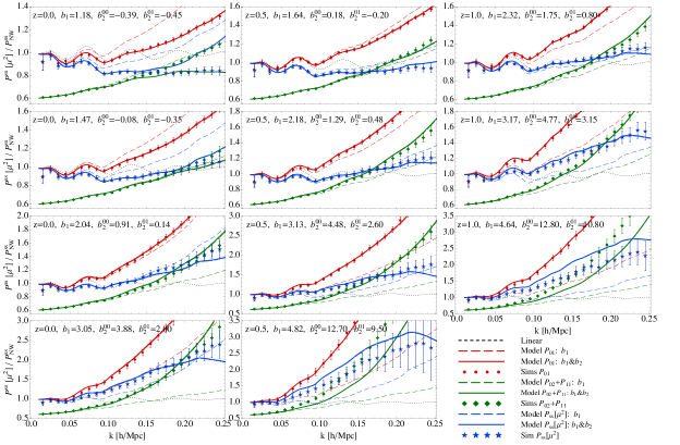
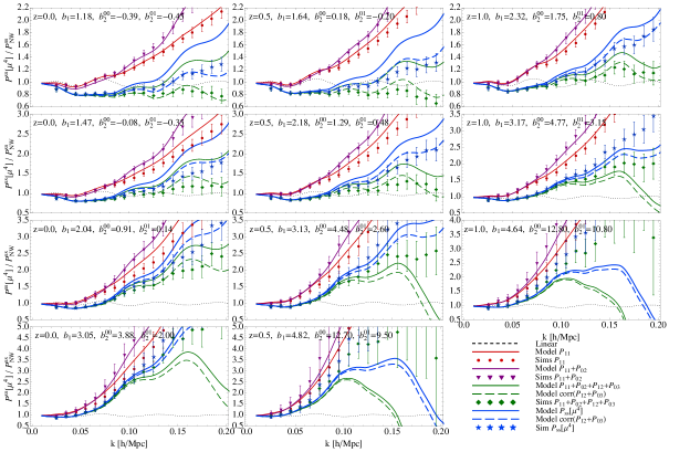
Refer to caption
Figure 12: Contribution of all the terms to μ2superscript𝜇2\mu^{2} part of redshift space power spectrum, for several mass bins at redshifts z=0.0𝑧0.0z=0.0, z=0.5𝑧0.5z=0.5 and z=1.0𝑧1.0z=1.0. We also show the contribution of P01subscript𝑃01P_{01} term (red) and P02+P11subscript𝑃02subscript𝑃11P_{02}+P_{11} term (green) to the total model (blue). P02+P11subscript𝑃02subscript𝑃11P_{02}+P_{11} term has been shifted up by 0.6. We compare the model results (solid lines) to the simulation measurements (points). Model where only linear b1subscript𝑏1b_{1} is used is also shown (dashed lines) for comparison. All the lines are divided by no-wiggle Kaiser μ2superscript𝜇2\mu^{2} term.
Refer to caption
Figure 13: Contribution of all the terms to μ4superscript𝜇4\mu^{4} part of redshift space power spectrum, for several mass bins at redshifts z=0.0𝑧0.0z=0.0, z=0.5𝑧0.5z=0.5 and z=1.0𝑧1.0z=1.0. We also show the contribution of P11subscript𝑃11P_{11} term (red), P02subscript𝑃02P_{02} term (purple), P12+P03subscript𝑃12subscript𝑃03P_{12}+P_{03} term (green) to the total model (blue). We compare the model results (solid lines) to the simulation measurements (points). We also show the results when the correction to P12+P03subscript𝑃12subscript𝑃03P_{12}+P_{03} term is added to the model (dashed lines), as discussed in section 2.7. All the lines are divided by no-wiggle Kaiser μ4superscript𝜇4\mu^{4} terms.
Refer to caption
Figure 14: Contribution to μ6superscript𝜇6\mu^{6} part of redshift space power spectrum, for two mass bins at redshifts z=0.0𝑧0.0z=0.0, z=0.5𝑧0.5z=0.5 and z=1.0𝑧1.0z=1.0. We show one loop PT result (solid lines) and compare to the simulation measurements (points). All the plots are divided by the linear predictions k2σv2PNWsuperscript𝑘2superscriptsubscript𝜎𝑣2subscript𝑃𝑁𝑊k^{2}\sigma_{v}^{2}P_{NW} with no BAO wiggles.

In [53] we resummed our model 3.1 to allow a continuation to higher powers of μ2superscript𝜇2\mu^{2}. In the dark matter case this procedure was not possible because of the small scale velocity dispersion, and because these small scale velocity dispersions appear with different amplitudes in contributing terms. This is because dark matter is distributed into halos of widely varying mass and different terms pick up different mass weightings: for example, some are additionally weighted by bias, some by higher powers of mass etc. (see [53] for details). In the case of halos we concluded above that our modeling gives a fairly good estimate of the velocity dispersion for all correlators, meaning that the small scale velocity dispersion is small and the velocity correlators are dominated by large scale velocity flows. However, in case of halos this procedure might be formally justified, but this only partially resums the series, leaving all of the other terms that do not contain velocity correlators untouched. Since velocity dispersion is much smaller in case of halos than it is for dark matter, terms that do not contain velocity dispersion are more relevant for halos in a relative sense. Since resummation is effecting only velocity dispersion terms one should not expect that this will then dramatically improve the overall performance of RSD model.

It is customary to expand the redshift-space power spectrum in terms of Legendre multipole moments

Pss(k,μ)=l=0,2,4,Plss(k)𝒫l(μ),superscript𝑃𝑠𝑠𝑘𝜇subscript𝑙024subscriptsuperscript𝑃𝑠𝑠𝑙𝑘subscript𝒫𝑙𝜇P^{ss}(k,\mu)=\sum_{l=0,2,4,\cdots}P^{ss}_{l}(k){\cal P}_{l}(\mu), (3.3)

where 𝒫l(μ)subscript𝒫𝑙𝜇{\cal P}_{l}(\mu) are ordinary Legendre polynomials and multipole moments, Plsssubscriptsuperscript𝑃𝑠𝑠𝑙P^{ss}_{l}, are given by

Plss(k)=(2l+1)01Pss(k,μ)𝒫l(μ)𝑑μ.subscriptsuperscript𝑃𝑠𝑠𝑙𝑘2𝑙1subscriptsuperscript10superscript𝑃𝑠𝑠𝑘𝜇subscript𝒫𝑙𝜇differential-d𝜇P^{ss}_{l}(k)=(2l+1)\int^{1}_{0}P^{ss}(k,\mu){\cal P}_{l}(\mu)d\mu~{}. (3.4)

In the RSD analysis it is common to model the monopole (l=0𝑙0l=0) and quadrupole (l=2𝑙2l=2) terms, since these contain most of the information on the angular structure of the correlations, although some information is also contained in the hexadecapole term (l=4𝑙4l=4), which we will not include here since it is dominated by μ6superscript𝜇6\mu^{6} terms that we do not explicitly model (although is present in our model through the resummation term).

In figures 15 and 16 we show monopole and quadrupole power spectra predictions. We show contributions to the multipoles as powers of μ𝜇\mu and compare all the results to the reference multipole data obtained from full simulation redshift space power spectra. We also show simulation results where only terms up to μ4superscript𝜇4\mu^{4} are considered. In the case of monopole we see that these two simulation results agree on scales larger than k(0.100.15)similar-to𝑘0.100.15k\sim(0.10-0.15)h/Mpc (depending on redshift and bias), but then start to deviate one from the other. These is especially apparent the case of the quadrupole, where we clearly see the difference in power when terms up to μ4superscript𝜇4\mu^{4} are considered, and the power when higher powers of μ𝜇\mu are also taken into account, i.e. terms proportional to μ6superscript𝜇6\mu^{6} and higher. We also show the result where one loop SPT prediction of μ6superscript𝜇6\mu^{6} term is added to the model. We see that better modelling of also these μ6superscript𝜇6\mu^{6} terms is necessary to achieve more precise results in total.
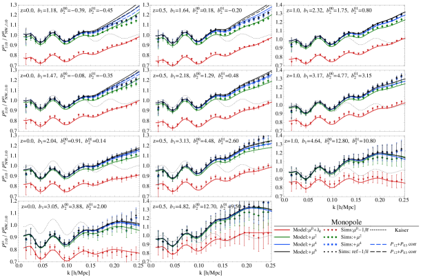
Refer to caption
Figure 15: Monopole (l=0𝑙0l=0) shown for several mass bins at redshifts z=0.0𝑧0.0z=0.0, z=0.5𝑧0.5z=0.5 and z=1.0𝑧1.0z=1.0. First the isotropic P00subscript𝑃00P_{00} part (in red) is shown and then we add the contributions of μ2superscript𝜇2\mu^{2} (green), μ4superscript𝜇4\mu^{4} (blue) and μ6superscript𝜇6\mu^{6} (black) part. Solid lines show the model presented in this paper and corresponding point marks simulation measurements of the same quantities. We also show the model (dashed lines) when the correction to P12+P03subscript𝑃12subscript𝑃03P_{12}+P_{03} term is added to the μ4superscript𝜇4\mu^{4} term, as discussed in section 2.7. Direct simulation measurements of monopole (black points) is also shown. All the lines and data are divided by the Kaiser no-wiggle monopole prediction.
Refer to caption
Figure 16: Quadrupole (l=2𝑙2l=2) shown for several mass bins at redshifts z=0.0𝑧0.0z=0.0, z=0.5𝑧0.5z=0.5 and z=1.0𝑧1.0z=1.0. We show μ2superscript𝜇2\mu^{2} part (in red) and then add the contributions of μ4superscript𝜇4\mu^{4} (blue) and μ6superscript𝜇6\mu^{6} (black) part. Solid lines show the model presented in this paper and corresponding point marks simulation measurements of the same quantities. We also show the model (dashed lines) when the correction to P12+P03subscript𝑃12subscript𝑃03P_{12}+P_{03} term is added to the μ4superscript𝜇4\mu^{4} term, as discussed in section 2.7. Direct simulation measurements of monopole (black points) is also shown. All the lines and data are divided by the Kaiser no-wiggle quadrupole prediction.

In figure 17 we show the angular dependence of model versus simulations for five angular bins, also known in the literature as clustering wedges. Similar techniques have recently been used in analysis of the correlation function (e.g. [63]). We show the model up to μ4superscript𝜇4\mu^{4}, with and without the correction on P03+P12subscript𝑃03subscript𝑃12P_{03}+P_{12} model and compare the results to the simulation measurements. We see that, as expected, the model is better for the case of low μ𝜇\mu since the expansion parameter of the distribution function approach is kvsubscript𝑘parallel-to𝑣k_{\parallel}v and by construction we have a very good model for real space power spectrum.
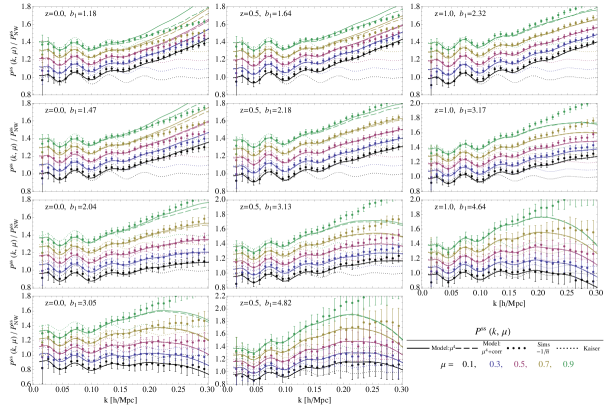
Refer to caption
Figure 17: Angular dependence of the RSD model for several mass bins at redshifts z=0.0𝑧0.0z=0.0, z=0.5𝑧0.5z=0.5 and z=1.0𝑧1.0z=1.0. We show the RSD model up to μ4superscript𝜇4\mu^{4} (solid lines), and μ6superscript𝜇6\mu^{6} (dashed lines). Simulation measurements (points) are also shown for each μ𝜇\mu bin. We also show the model when the correction to P12+P03subscript𝑃12subscript𝑃03P_{12}+P_{03} term is added to the μ4superscript𝜇4\mu^{4} term (dashed line), as discussed in section 2.7. All the lines and data are divided by the Kaiser no-wiggle predictions. Results for each angle bin are offset for a constant value for a better overview.

4 Correlation function

Our model was built in Fourier space, but we can also look at its performance in configuration space. To get the correlation function we Fourier transform the redshift space power spectra

ξss(s)superscript𝜉𝑠𝑠s\displaystyle\xi^{ss}(\textbf{s}) =d3q(2π)3Pss(q)eiqsabsentsuperscript𝑑3𝑞superscript2𝜋3superscript𝑃𝑠𝑠qsuperscript𝑒𝑖qs\displaystyle=\int{\frac{d^{3}q}{(2\pi)^{3}}~{}P^{ss}(\textbf{q})e^{-i\textbf{q}\cdot\textbf{s}}}
=ξ0(s)𝒫0(ν)+ξ2(s)𝒫2(ν)+ξ4(s)𝒫4(ν)absentsubscript𝜉0𝑠subscript𝒫0𝜈subscript𝜉2𝑠subscript𝒫2𝜈subscript𝜉4𝑠subscript𝒫4𝜈\displaystyle=\xi_{0}(s){\cal P}_{0}(\nu)+\xi_{2}(s){\cal P}_{2}(\nu)+\xi_{4}(s){\cal P}_{4}(\nu) (4.1)

where we used first four ordinary Legendre polynomials, 𝒫0(ν)=1subscript𝒫0𝜈1{\cal P}_{0}(\nu)=1, 𝒫2(ν)=(3ν21)/2subscript𝒫2𝜈3superscript𝜈212{\cal P}_{2}(\nu)=(3\nu^{2}-1)/2 and 𝒫4(ν)=(35ν430ν2+3)/8subscript𝒫4𝜈35superscript𝜈430superscript𝜈238{\cal P}_{4}(\nu)=(35\nu^{4}-30\nu^{2}+3)/8, and ν𝜈\nu is the cosine of the angle between s and line of sight. Expansion coefficients are given by spherical Bessel function jlsubscript𝑗𝑙j_{l} moments of the power spectra

ξl(s)=ilq2dq2π2WR(q)Plss(q)jl(qs).subscript𝜉𝑙𝑠superscript𝑖𝑙superscript𝑞2𝑑𝑞2superscript𝜋2subscript𝑊𝑅𝑞subscriptsuperscript𝑃𝑠𝑠𝑙𝑞subscript𝑗𝑙𝑞𝑠\displaystyle\xi_{l}(s)=i^{l}\int{\frac{q^{2}dq}{2\pi^{2}}~{}W_{R}(q)P^{ss}_{l}(q)j_{l}(qs)}. (4.2)

However, many of our PT model predictions strongly diverge from simulations at high k𝑘k, a well known problem of PT. To cure this we introduce the window function W(qR)𝑊𝑞𝑅W(qR) with smoothing radius R𝑅R, which reduces the importance of high k𝑘k contributions to the correlation function. For the smoothing W(qR)𝑊𝑞𝑅W(qR) function we use the simple Gaussian filter. This suppresses the amplitude of the correlation function, and the effect is stronger as we approach smaller scales. We choose the value for which the filter effects on scales larger than s=5Mpc/h𝑠5𝑀𝑝𝑐s=5Mpc/h are small and are not noticeable in the figures 18 and 19 presented bellow. In principle stricter criteria could be implemented here to quantify these effects, but for our purposes this is not of the crucial importance. We find the value to be R=1.0h/Mpc𝑅1.0𝑀𝑝𝑐R=1.0h/Mpc for both monopole and quadrupole case. In figures 18 and 19 we show monopole and quadrupole predictions in configuration space, obtained by Fourier transforming the model presented in this work. We show the results for several mass bins and redshifts and compare them to the N-body simulation measurements. We note that the model is not supposed to be compared against simulations below s=10Mpc/h𝑠10𝑀𝑝𝑐s=10Mpc/h because of the artificial smoothing of the model against simulations. In principle we could have inserted the smoothing also into the simulations, but for this procedure a broad range of scales of the correlation function measurements is needed.
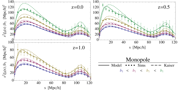
Refer to caption
Figure 18: Monopole of redshift-space correlation function for several mass bins at redshifts z=0.0𝑧0.0z=0.0, z=0.5𝑧0.5z=0.5 and z=1.0𝑧1.0z=1.0. We show the results of model presented in this work (solid lines) linear theory predictions (dashed lines) and halo simulation measurements (points). Results are shown for the same mass bins as in previous plots (upper line represents the highest bias and lower line represents the lowest bias, respectively).

5 Conclusions

In this paper we continue the studies of distribution function approach to redshift space distortions (RSD), applying Eulerian perturbation theory (PT) to the case of dark matter halos. In this formalism the RSD power spectrum is decomposed into moments of distribution function and our goal is to model these contributing terms using the perturbation theory and Eulerian biasing model. We work at 1-loop level in PT, requiring us to introduce 3 additional biasing parameters, of which we find that one, the tidal tensor bias bssubscript𝑏𝑠b_{s}, turns out not to be important if one assumes its amplitude is given by the bispectrum analysis [55, 39]. The remaining two nonlinear bias parameters are the local quadratic bias b2subscript𝑏2b_{2} and the non-local 3rd order bias b3,nlsubscript𝑏3𝑛𝑙b_{3,nl}. These two have similar scale dependence with k𝑘k, at least over a limited range of k<0.15h/Mpc𝑘0.15𝑀𝑝𝑐k<0.15h/Mpc, but have different amplitudes in the density-density correlator P00hmsubscriptsuperscript𝑃𝑚00P^{hm}_{00} relative to the density-momentum correlator P01(hh)subscriptsuperscript𝑃01P^{(hh)}_{01}. One can thus parametrize these nonlinear biases with 2 independent effective 2nd order bias terms. Simple coevolution theory predicts that the nonlinear biasing should be weaker in density-momentum relative to density-density [59], and our results confirm this prediction.

We require that our biasing scheme is consistent with other statistics, in particular the halo-dark matter density cross-correlation P00hmsubscriptsuperscript𝑃𝑚00P^{hm}_{00} [59]. We also assume that the tidal tensor bias bssubscript𝑏𝑠b_{s} is consistent with the bispectrum [40, 55]. We thus start by modelling the halo matter cross correlation term P00(hm)subscriptsuperscript𝑃𝑚00P^{(hm)}_{00} where we fit for effective b200subscriptsuperscript𝑏002b^{00}_{2} values, combining all the nonlinear bias terms into one. However, since the statistic that enters the RSD is the halo-halo density correlator P00hhsuperscriptsubscript𝑃00P_{00}^{hh}, this means we also need to describe the stochasticity Λ(k)=P00hh2b1P00hm+b12P00mmΛ𝑘superscriptsubscript𝑃002subscript𝑏1superscriptsubscript𝑃00𝑚superscriptsubscript𝑏12superscriptsubscript𝑃00𝑚𝑚\Lambda(k)=P_{00}^{hh}-2b_{1}P_{00}^{hm}+b_{1}^{2}P_{00}^{mm}. Detailed modeling of this term is complicated, and is related to halo exclusion and nonlinear biasing [58]. Since our goal is to study RSD we do not attempt to develop a more detailed model of this term and instead we simply parametrize it with a simple power law expression. For the most of the mass bins that were considered we encounter sub-Poissonian stochasticity. We next turn to the modelling of higher momentum correlations, for which the nonlinear contributions of bias at one loop level enter explicitly only in the P01(hh)subscriptsuperscript𝑃01P^{(hh)}_{01} term. We find the values of effective b201subscriptsuperscript𝑏012b^{01}_{2} that reproduce the simulation measurements. We have argued that at the level of 1-loop calculations this approach is consistent, as we have both quadratic local bias b2subscript𝑏2b_{2} and cubic non-local bias b3,nlsubscript𝑏3𝑛𝑙b_{3,nl} entering at the same order, but with differing coefficients in P00hhsuperscriptsubscript𝑃00P_{00}^{hh} versus P01hhsuperscriptsubscript𝑃01P_{01}^{hh}.

Refer to caption
Figure 19: Same as figure 18 but for quadrupole moment of redshift-space correlation function. Results for each mass bin are offset by a constant value (15 (Mpc/h)2superscriptMpc/h2(\text{Mpc/h})^{2}) relative to the lowest (blue) bias.

In addition to biasing PT approach also computes dark matter clustering. However, in previous work [53] we found that PT does not do a good job in predicting the dark matter correlators: this is a well known property of PT for density-density and density-velocity correlations (e.g. [23]), which also holds for higher order density weighted velocity moment correlators. As a result we use the dark matter correlators as presented in [53], which were a combination of simulation measurements and perturbation theory calculations. We divide the halo correlators into the dark matter part and the remaining part, which depends on linear and nonlinear bias parameters. We use PT to compute both linear and nonlinear biasing contributions to the halo correlators. For the dark matter part, we use P00subscript𝑃00P_{00}, P01subscript𝑃01P_{01}, P11subscript𝑃11P_{11} and Pδθsubscript𝑃𝛿𝜃P_{\delta\theta} as given by the dark matter simulations. Ideally this part will also be eventually replaced by PT, but since our goal here is not the dark matter modeling but the halo modeling we do not investigate it further.

The dominant term to RSD is the μ2superscript𝜇2\mu^{2} term and its dominant contribution is the halo momentum density correlated with the halo density. Two other terms contribute to μ2superscript𝜇2\mu^{2}, the vector part of the halo momentum density- halo momentum density correlation P11hhsuperscriptsubscript𝑃11P_{11}^{hh}, and the scalar part of halo kinetic energy density - halo density correlation P02hhsuperscriptsubscript𝑃02P_{02}^{hh}. We find that they affect RSD at a 10% level already at k0.05h/Mpcsimilar-to𝑘0.05hMpck\sim 0.05{\rm h/Mpc} for most of the mass bins we consider. The halo kinetic energy density- halo density correlation term P02subscript𝑃02P_{02} is the dominant nonlinear effect, and is negative at all k𝑘k and thus reduces the total μ2superscript𝜇2\mu^{2} power. It is related to the Fingers-of-God (FoG) effect, since this term contains velocity dispersion term. However, unlike the velocity dispersion inside the halos, which dominates FoG for dark matter, this effect is generated by the large scale velocity flows which cancel out with P11subscript𝑃11P_{11} term on small scales. As a result there are no velocity dispersion effects on small scales.

The next angular term has μ4superscript𝜇4\mu^{4} dependence and there are seven terms that contribute to the total power spectrum, of which one, scalar part of P11(hh)subscriptsuperscript𝑃11P^{(hh)}_{11}, contains a linear order contribution that does not vanish on large scales. Modelling these terms has proven to be even more difficult than lower order terms, but certain level of success has been achieved compared to the simulations over a limited dynamic range, with errors of about 10% at k0.1h/Mpcsimilar-to𝑘0.1hMpck\sim 0.1{\rm h/Mpc} at z=0𝑧0z=0. All these terms exhibit very strong scale dependence, which we can reproduce in our model, which should be viewed as a success since there are no free parameters used. Nevertheless, some of the terms also have a considerable error, specially in P03hh+P12hhsuperscriptsubscript𝑃03superscriptsubscript𝑃12P_{03}^{hh}+P_{12}^{hh}, and as a result we do not succeed in modeling accurately the modes above k0.15h/Mpcsimilar-to𝑘0.15𝑀𝑝𝑐k\sim 0.15h/Mpc.

Our ultimate goal is to develop an accurate RSD model that can be applied to observations, but this was not the primary focus of this work. Instead, here we focused on asking whether we can model all the diferent halo density weighted powers of velocity using a consistent halo biasing model at 1-loop level. We emphasize that all of our biasing parameters are physically motivated: indeed, in most cases they can be predicted from a biasing model [55, 39, 59] and all of the bias parameters exhibit a simple halo mass dependence that can be used as a prior when applying these models to the real data. We introduced no arbitrary velocity dispersion parameters, like those needed in models of most previous work on the subject [14, 20]. This is because when it comes to halos there is no small scale velocity dispersion, as the halos centers are at rest with respect to the local center of mass. All velocity dispersion effects come from large scale velocities which are fully modeled in our approach using PT. We do not compute higher order velocity effects beyond μ4superscript𝜇4\mu^{4} and instead we propose a simple resummation ansatz that should approximately capture these terms. We have achieved some level of accuracy with our modeling, but a 1% precision, needed for current and future RSD surveys, can only be achieved up to k0.15h/Mpcsimilar-to𝑘0.15𝑀𝑝𝑐k\sim 0.15h/Mpc. We have seen that the nonlinear effects at that k𝑘k are at 10-20% level or larger and rapidly growing towards higher k𝑘k, making it difficult to significantly improve the model beyond what was achieved here. Performance of the presented RSD model in determining the cosmological parameter and comparison to some of the other models will be studied in [64].

Successful modeling of halo velocity statistics is just one ingredient of the complete RSD model. We observe galaxies, not dark matter halos, and our analysis remains to be extended to galaxies. We saw previously that for dark matter we had to introduce small scale velocity dispersion to model FoG effects in RSD and we expect the same to be true for galaxies. Nevertheless, separating halo biasing effects, the focus of this work, from FoG effects is an important step towards the complete RSD model. The treatment of FoG we used for dark matter, based on the halo model for computing velocity dispersion, should also be applicable to galaxies. We plan to address this in the future work.

Acknowledgments

We would like to thank Patrick McDonald, Shun Saito, Tobias Baldauf, Jonathan Blazek, Masanori Sato, Jaiyul Yoo and Nico Hamaus for useful discussions and comments. ZV would like to thank the Berkeley Center for Cosmological Physics and the Lawrence Berkeley Laboratory for their hospitality. This work is supported by the DOE, the Swiss National Foundation under contract 200021-116696/1 and WCU grant R32-10130. V.D. acknowledges support by the Swiss National Science Foundation. The simulations were performed on the ZBOX3 supercomputer of the Institute for Theoretical Physics at the University of Zürich. For making some of the plots in this paper LevelScheme package [65] has been used.

References

  • [1] N. Kaiser, Clustering in real space and in redshift space, Mon. Not. Roy. Astron. Soc. 227 (1987) 1–27.
  • [2] A. Hamilton, Linear redshift distortions: A Review, astro-ph/9708102. Published in The Evolving Universe. Edited by D. Hamilton, Kluwer Academic, 1998, p. 185-275.
  • [3] J. Jackson, Fingers of God, Mon.Not.Roy.Astron.Soc. 156 (1972) 1, [arXiv:0810.3908].
  • [4] S. Cole, K. B. Fisher, and D. H. Weinberg, Fourier analysis of redshift space distortions and the determination of Omega, Mon.Not.Roy.Astron.Soc. 267 (1994) 785, [astro-ph/9308003].
  • [5] M. White, Y.-S. Song, and W. J. Percival, Forecasting Cosmological Constraints from Redshift Surveys, Mon.Not.Roy.Astron.Soc. 397 (2008) 1348–1354, [arXiv:0810.1518].
  • [6] P. McDonald and U. Seljak, How to measure redshift-space distortions without sample variance, JCAP 0910 (2009) 007, [arXiv:0810.0323].
  • [7] K. Yamamoto, T. Sato, and G. Huetsi, Testing general relativity with the multipole spectra of the SDSS luminous red galaxies, Prog.Theor.Phys. 120 (2008) 609–614, [arXiv:0805.4789].
  • [8] B. A. Reid, W. J. Percival, D. J. Eisenstein, L. Verde, D. N. Spergel, et. al., Cosmological Constraints from the Clustering of the Sloan Digital Sky Survey DR7 Luminous Red Galaxies, Mon.Not.Roy.Astron.Soc. 404 (2010) 60–85, [arXiv:0907.1659].
  • [9] SDSS Collaboration Collaboration, W. J. Percival et. al., Baryon Acoustic Oscillations in the Sloan Digital Sky Survey Data Release 7 Galaxy Sample, Mon.Not.Roy.Astron.Soc. 401 (2010) 2148–2168, [arXiv:0907.1660].
  • [10] E. A. Kazin, M. R. Blanton, R. Scoccimarro, C. K. McBride, and A. A. Berlind, Regarding the Line-of-Sight Baryonic Acoustic Feature in the Sloan Digital Sky Survey and Baryon Oscillation Spectroscopic Survey Luminous Red Galaxy Samples, Astrophys.J. 719 (2010) 1032–1044, [arXiv:1004.2244].
  • [11] G. M. Bernstein and Y.-C. Cai, Cosmology without cosmic variance, arXiv:1104.3862.
  • [12] B. A. Reid, L. Samushia, M. White, W. J. Percival, M. Manera, et. al., The clustering of galaxies in the SDSS-III Baryon Oscillation Spectroscopic Survey: measurements of the growth of structure and expansion rate at z=0.57 from anisotropic clustering, arXiv:1203.6641.
  • [13] L. Casarini, S. A. Bonometto, S. Borgani, K. Dolag, G. Murante, et. al., Tomographic weak lensing shear spectra from large N-body and hydrodynamical simulations, arXiv:1203.5251.
  • [14] R. Scoccimarro, Redshift-space distortions, pairwise velocities and nonlinearities, Phys.Rev. D70 (2004) 083007, [astro-ph/0407214].
  • [15] J. R. Shaw and A. Lewis, Non-linear Redshift-Space Power Spectra, Phys.Rev. D78 (2008) 103512, [arXiv:0808.1724].
  • [16] T. Okumura and Y. Jing, Systematic Effects on Determination of the Growth Factor from Redshift-space Distortions, Astrophys.J. 726 (2011) 5, [arXiv:1004.3548].
  • [17] A. Taruya, T. Nishimichi, and S. Saito, Baryon Acoustic Oscillations in 2D: Modeling Redshift-space Power Spectrum from Perturbation Theory, Phys.Rev. D82 (2010) 063522, [arXiv:1006.0699].
  • [18] E. Jennings, C. M. Baugh, and S. Pascoli, Modelling redshift space distortions in hierarchical cosmologies, Mon.Not.Roy.Astron.Soc. 410 (2011) 2081, [arXiv:1003.4282].
  • [19] J. Tang, I. Kayo, and M. Takada, Likelihood reconstruction method of real-space density and velocity power spectra from a redshift galaxy survey, arXiv:1103.3614.
  • [20] A. Taruya, T. Nishimichi, and F. Bernardeau, Precision modeling of redshift-space distortions from multi-point propagator expansion, arXiv:1301.3624.
  • [21] A. Vallinotto and E. V. Linder, Redshift Space Distortion Reconstruction, arXiv:1307.2906.
  • [22] F. Bernardeau, S. Colombi, E. Gaztanaga, and R. Scoccimarro, Large scale structure of the universe and cosmological perturbation theory, Phys.Rept. 367 (2002) 1–248, [astro-ph/0112551].
  • [23] J. Carlson, M. White, and N. Padmanabhan, A critical look at cosmological perturbation theory techniques, Phys. Rev. D80 (2009) 043531, [arXiv:0905.0479].
  • [24] M. Crocce and R. Scoccimarro, Renormalized cosmological perturbation theory, Phys.Rev. D73 (2006) 063519, [astro-ph/0509418].
  • [25] M. Crocce and R. Scoccimarro, Memory of initial conditions in gravitational clustering, Phys.Rev. D73 (2006) 063520, [astro-ph/0509419].
  • [26] M. Crocce and R. Scoccimarro, Nonlinear Evolution of Baryon Acoustic Oscillations, Phys.Rev. D77 (2008) 023533, [arXiv:0704.2783].
  • [27] T. Matsubara, Resumming Cosmological Perturbations via the Lagrangian Picture: One-loop Results in Real Space and in Redshift Space, Phys.Rev. D77 (2008) 063530, [arXiv:0711.2521].
  • [28] T. Matsubara, Nonlinear perturbation theory with halo bias and redshift-space distortions via the Lagrangian picture, Phys.Rev. D78 (2008) 083519, [arXiv:0807.1733].
  • [29] P. McDonald, Dark matter clustering: a simple renormalization group approach, Phys.Rev. D75 (2007) 043514, [astro-ph/0606028].
  • [30] A. Taruya and T. Hiramatsu, A Closure Theory for Non-linear Evolution of Cosmological Power Spectra, arXiv:0708.1367.
  • [31] M. Pietroni, Flowing with Time: a New Approach to Nonlinear Cosmological Perturbations, JCAP 0810 (2008) 036, [arXiv:0806.0971].
  • [32] P. Valageas, A new approach to gravitational clustering: a path-integral formalism and large-n expansions, Astron.Astrophys. 421 (2004) 23–40, [astro-ph/0307008].
  • [33] A. Taruya, T. Nishimichi, S. Saito, and T. Hiramatsu, Non-linear Evolution of Baryon Acoustic Oscillations from Improved Perturbation Theory in Real and Redshift Spaces, Phys.Rev. D80 (2009) 123503, [arXiv:0906.0507].
  • [34] A. Taruya, F. Bernardeau, T. Nishimichi, and S. Codis, RegPT: Direct and fast calculation of regularized cosmological power spectrum at two-loop order, Phys.Rev. D86 (2012) 103528, [arXiv:1208.1191].
  • [35] S. Anselmi and M. Pietroni, Nonlinear Power Spectrum from Resummed Perturbation Theory: a Leap Beyond the BAO Scale, JCAP 1212 (2012) 013, [arXiv:1205.2235].
  • [36] M. Crocce, R. Scoccimarro, and F. Bernardeau, MPTbreeze: A fast renormalized perturbative scheme, arXiv:1207.1465.
  • [37] P. McDonald, Clustering of dark matter tracers: Renormalizing the bias parameters, Phys.Rev. D74 (2006) 103512, [astro-ph/0609413].
  • [38] P. McDonald and A. Roy, Clustering of dark matter tracers: generalizing bias for the coming era of precision LSS, JCAP 0908 (2009) 020, [arXiv:0902.0991].
  • [39] K. C. Chan, R. Scoccimarro, and R. K. Sheth, Gravity and Large-Scale Non-local Bias, Phys.Rev. D85 (2012) 083509, [arXiv:1201.3614].
  • [40] K. C. Chan and R. Scoccimarro, Halo Sampling, Local Bias and Loop Corrections, arXiv:1204.5770.
  • [41] A. J. Nishizawa, M. Takada, and T. Nishimichi, Perturbation theory for nonlinear halo power spectrum: the renormalized bias and halo bias, arXiv:1212.4025.
  • [42] J. L. Tinker, Redshift-Space Distortions with the Halo Occupation Distribution II: Analytic Model, Mon.Not.Roy.Astron.Soc. 374 (2007) 477–492, [astro-ph/0604217].
  • [43] T. Nishimichi and A. Taruya, Baryon Acoustic Oscillations in 2D II: Redshift-space halo clustering in N-body simulations, Phys.Rev. D84 (2011) 043526, [arXiv:1106.4562].
  • [44] T. Matsubara, Nonlinear Perturbation Theory Integrated with Nonlocal Bias, Redshift-space Distortions, and Primordial Non-Gaussianity, Phys.Rev. D83 (2011) 083518, [arXiv:1102.4619].
  • [45] T. Matsubara, Deriving an Accurate Formula of Scale-dependent Bias with Primordial Non-Gaussianity: An Application of the Integrated Perturbation Theory, Phys.Rev. D86 (2012) 063518, [arXiv:1206.0562].
  • [46] B. A. Reid and M. White, Towards an accurate model of the redshift space clustering of halos in the quasilinear regime, arXiv:1105.4165.
  • [47] M. Sato and T. Matsubara, Nonlinear Biasing and Redshift-Space Distortions in Lagrangian Resummation Theory and N-body Simulations, Phys.Rev. D84 (2011) 043501, [arXiv:1105.5007].
  • [48] H. Gil-Marin, C. Wagner, L. Verde, C. Porciani, and R. Jimenez, Perturbation theory approach for the power spectrum: from dark matter in real space to haloes in redshift space, JCAP 1211 (2012) 029, [arXiv:1209.3771].
  • [49] J. Carlson, B. Reid, and M. White, Convolution Lagrangian perturbation theory for biased tracers, arXiv:1209.0780.
  • [50] L. Wang, B. Reid, and M. White, An analytic model for redshift-space distortions, Mon. Not. R. Astron. Soc. (2013) [arXiv:1306.1804].
  • [51] U. Seljak and P. McDonald, Distribution function approach to redshift space distortions, arXiv:1109.1888.
  • [52] T. Okumura, U. Seljak, P. McDonald, and V. Desjacques, Distribution function approach to redshift space distortions: N-body simulations, arXiv:1109.1609.
  • [53] Z. Vlah, U. Seljak, P. McDonald, T. Okumura, and T. Baldauf, Distribution function approach to redshift space distortions. Part IV: perturbation theory applied to dark matter, arXiv:1207.0839.
  • [54] T. Okumura, U. Seljak, and V. Desjacques, Distribution function approach to redshift space distortions, Part III: halos and galaxies, arXiv:1206.4070.
  • [55] T. Baldauf, U. Seljak, V. Desjacques, and P. McDonald, Evidence for Quadratic Tidal Tensor Bias from the Halo Bispectrum, arXiv:1201.4827.
  • [56] V. Desjacques and R. K. Sheth, Redshift space correlations and scale-dependent stochastic biasing of density peaks, Phys.Rev. D81 (2010) 023526, [arXiv:0909.4544].
  • [57] V. Desjacques, M. Crocce, R. Scoccimarro, and R. K. Sheth, Modeling scale-dependent bias on the baryonic acoustic scale with the statistics of peaks of Gaussian random fields, Phys.Rev. D82 (2010) 103529, [arXiv:1009.3449].
  • [58] T. Baldauf, U. Seljak, R. E. Smith, N. Hamaus, and V. Desjacques, Halo Stochasticity from Exclusion and non-linear Clustering, arXiv:1305.2917.
  • [59] S. Saito, et. al., In preparation, .
  • [60] N. Hamaus, U. Seljak, V. Desjacques, R. E. Smith, and T. Baldauf, Minimizing the Stochasticity of Halos in Large-Scale Structure Surveys, Phys.Rev. D82 (2010) 043515, [arXiv:1004.5377].
  • [61] D. J. Eisenstein and W. Hu, Baryonic Features in the Matter Transfer Function, Astrophys. J. 496 (1998) 605, [astro-ph/9709112].
  • [62] V. Desjacques, Baryon acoustic signature in the clustering of density maxima, Phys.Rev. D78 (2008) 103503, [arXiv:0806.0007].
  • [63] E. A. Kazin, A. G. Sanchez, A. J. Cuesta, F. Beutler, C.-H. Chuang, et. al., The Clustering of Galaxies in the SDSS-III Baryon Oscillation Spectroscopic Survey: Measuring H(z) and D(z) at z = 0.57 with Clustering Wedges, arXiv:1303.4391.
  • [64] J. Blazek, et. al., In preparation, .
  • [65] M. Caprio, LevelScheme: A level scheme drawing and scientific figure preparation system for Mathematica, Computer Physics Communications 171 (Sept., 2005) 107–118, [physics/0].